Embed Size (px)
Citation preview

11
The The PPCCPP starting point starting point

22
OverviewOverview
In this lecture we’ll present the In this lecture we’ll present the Quadratic SolvabilityQuadratic Solvability problem. problem.
We’ll see this problem is closely We’ll see this problem is closely related to related to PCPPCP..
And even use it to prove a (very very And even use it to prove a (very very weak...) weak...) PCPPCP characterization of characterization of NPNP..

33
Quadratic SolvabilityQuadratic Solvability
Def: (QS[D, Def: (QS[D, ]):]): InstanceInstance:: a set of a set of nn quadratic equations over quadratic equations over
with at most with at most DD variables each. variables each.ProblemProblem:: to find if there is a common solution. to find if there is a common solution.
or equally: a set of dimension Dtotal-degree 2 polynomials
Example: =Z2; D=1
y = 0
x 2 + x = 0
x 2 + 1 = 0
1 1
1
0

44
SolvabilitySolvability
A generalization of this problem:A generalization of this problem:
Def: (Solvability[D, Def: (Solvability[D, ]):]):
InstanceInstance:: a set of a set of n n polynomials over polynomials over with with at most at most DD variables. Each polynomial has variables. Each polynomial has degree-bound degree-bound n n in each one of the in each one of the variables. variables.
ProblemProblem:: to find if there is a common root. to find if there is a common root.
55
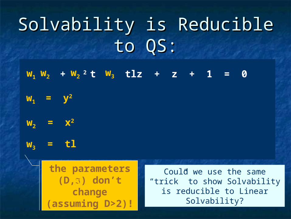
Solvability is Reducible to Solvability is Reducible to QS:QS:
y2 x2 + x2 t + tlz + z + 1 = 0w1
w1 = y2
w2
w2 = x2
w3
w3 = tl
w2
Could we use the same “trick” to show Solvability is reducible
to Linear Solvability?
the parameters (D,) don’t
change (assuming
D>2)!

66
QS is NP-hardQS is NP-hardLet us prove that QS is NP-hard by reducing Let us prove that QS is NP-hard by reducing 3-SAT 3-SAT
to it:to it:
(123)...(m/3-2m/3-1m/3) where each literal i{xj,xj}1jn
Def: (3-SAT):Def: (3-SAT): InstanceInstance:: a a 3CNF3CNF formula. formula. ProblemProblem:: to decide if this formula is satisfiable. to decide if this formula is satisfiable.

77
Given an instance of Given an instance of 3-SAT3-SAT, use the following , use the following transformation on each clause:transformation on each clause:
QS is NP-hardQS is NP-hard
xxii 1-x1-xii
xxii xxii
( ( ii i+1i+1 i+2i+2 ) ) Tr[ Tr[ ii ] * Tr[ ] * Tr[ i+1i+1 ] * Tr[ ] * Tr[ i+2i+2 ] ]
The corresponding instance of The corresponding instance of SolvabilitySolvability is the set is the set of all resulting polynomials (which, assuming the of all resulting polynomials (which, assuming the variables are only assigned Boolean values, is variables are only assigned Boolean values, is equivalent)equivalent)
88
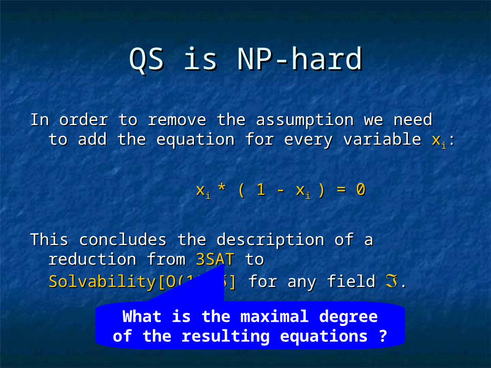
QS is NP-hardQS is NP-hard
In order to remove the assumption we need to add In order to remove the assumption we need to add the equation for every variable the equation for every variable xxii::
xxi i * ( 1 - x* ( 1 - xi i ) = 0) = 0
This concludes the description of a reduction from This concludes the description of a reduction from 3SAT3SAT to to Solvability[O(1),Solvability[O(1),]] for any field for any field ..
What is the maximal degree of the resulting equations ?
99
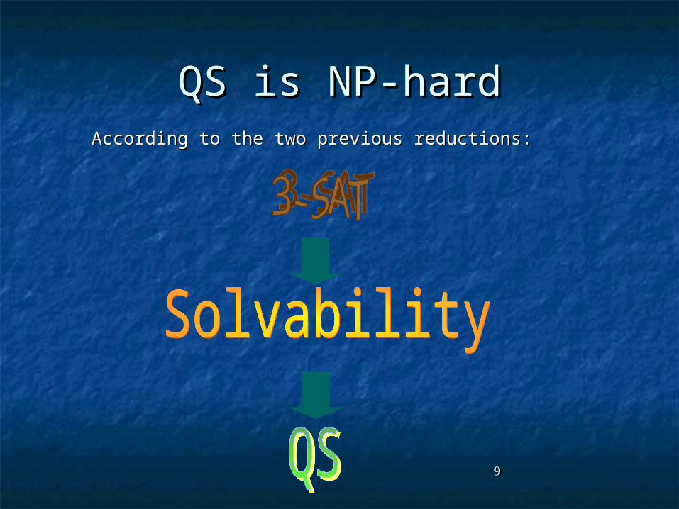
QS is NP-hardQS is NP-hardAccording to the two previous reductions:According to the two previous reductions:

1010
Gap-QSGap-QS
Def: (Gap-QS[D, Def: (Gap-QS[D, ,,]):]):
InstanceInstance:: a set of a set of nn quadratic equations over quadratic equations over with with at most at most DD variables each. variables each.
ProblemProblem:: to distinguish between the following two to distinguish between the following two cases:cases:
There is a common solutionThere is a common solution
No more than an No more than an fraction of the equations fraction of the equations can be satisfied simultaneously. can be satisfied simultaneously.

1111
Def:Def:
LLPCP[PCP[DD,,VV, , ]] if there is a polynomial time if there is a polynomial time algorithm, which for any input algorithm, which for any input xx, produces, produces a set a set of efficient Boolean functions over variables of of efficient Boolean functions over variables of range range 22VV,, each depending on at mosteach depending on at most DD variables variables so that:so that:
xxLL iff there exits an assignment to the variables, iff there exits an assignment to the variables, which satisfies all the functionswhich satisfies all the functions
xxLL iff no assignment can satisfy more than an iff no assignment can satisfy more than an --fraction of the functions.fraction of the functions.
Gap-QS and PCPGap-QS and PCP
Gap-QS[Gap-QS[DD,,,,]] PCP[ PCP[DD,,log|log|||,,]]
Gap-QS[D,,]
quadratic equations system
For each quadratic polynomial pi(x1,...,xD), add the Boolean
function i(a1,...,aD)pi(a1,...,aD)=0the variables
of the input system
values in

1212
Gap-QS and PCPGap-QS and PCP
Therefore, every language which is Therefore, every language which is efficiently reducible to Gap-QS[efficiently reducible to Gap-QS[DD,,,,] is ] is also in also in PCP[PCP[DD,,log|log|||,,]]..
Thus, proving Gap-QS[Thus, proving Gap-QS[DD,,,,] is ] is NP-hardNP-hard, , also proves the also proves the PCP[PCP[DD,,log|log|||,,] ] characterization of characterization of NPNP..
And indeed our goal henceforth will be And indeed our goal henceforth will be proving Gap-QS[proving Gap-QS[DD,,,,] is ] is NP-hardNP-hard for the for the best best DD, , and and we can. we can.
1313
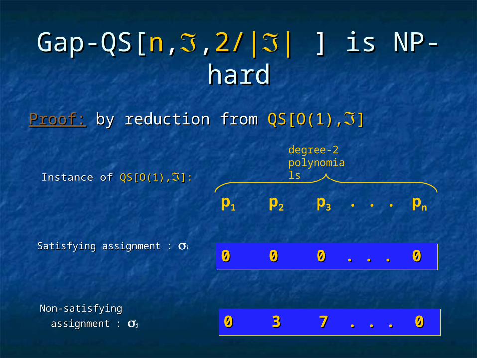
Gap-QS[Gap-QS[nn,,,,2/|2/||| ]] is NP-hard is NP-hard
Proof:Proof: by reduction from by reduction from QS[O(1),QS[O(1),]]
p1 p2 p3 . . . pn
degree-2 polynomials Instance of Instance of QS[O(1),QS[O(1),]:]:
Satisfying assignment : Satisfying assignment : i
00 00 0 . . .0 . . . 0000 00 0 . . .0 . . . 00
Non-satisfying assignment : Non-satisfying assignment :
j 00 33 7 . . .7 . . . 0000 33 7 . . .7 . . . 00
1414
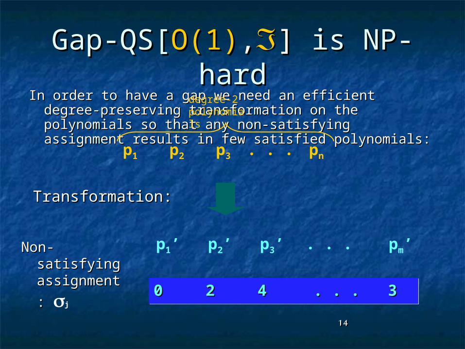
Gap-QS[Gap-QS[O(1)O(1),,]] is NP-hard is NP-hardIn order to have a gap we need an efficient degree-In order to have a gap we need an efficient degree-
preserving transformation on the polynomials so preserving transformation on the polynomials so that any non-satisfying assignment results in few that any non-satisfying assignment results in few satisfied polynomials:satisfied polynomials:p1 p2 p3 . . . pn
degree-2 polynomials
p1’ p2’ p3’ . . . pm’
Transformation:Transformation:
Non-Non-satisfying satisfying assignment assignment
: : j
00 22 4 . . . 34 . . . 300 22 4 . . . 34 . . . 3

1515
Gap-QS[Gap-QS[O(1)O(1),,]] is NP-hard is NP-hard
For such an efficient degree-preserving For such an efficient degree-preserving transformation transformation EE it must hold that: it must hold that:
n m
n m
1)E(0 ) 0
2) v 0 . (E(v),0 ) 1 2/
Thus Thus EE is an error correcting code ! is an error correcting code !
We shall now see examples of degree-preserving transformations We shall now see examples of degree-preserving transformations which are also error correcting codes:which are also error correcting codes:
1616
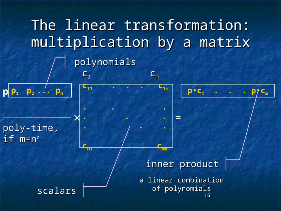
The linear transformation: The linear transformation: multiplication by a matrixmultiplication by a matrix
p1 p2 ... pn
c11 . . . c1m
. . .
. . .
. . .
cn1 . . . cnm
p
cc1 . . . 1 . . . ccmm
p•c1 . . . p•cm
=
scalarsscalars
polynomialspolynomials
inner productinner product
a linear combination of a linear combination of polynomialspolynomials
poly-time, if poly-time, if m=nm=ncc

1717
The linear transformation: The linear transformation: multiplication by a matrixmultiplication by a matrix
e1 e2 ... en
c11 . . . c1m
. . .
. . .
. . .
cn1 . . . cnm
c1 . . . cm
•c1 . . . •cm
=
the values of the polynomials under some the values of the polynomials under some assignmentassignment
the values of the new polynomials under the values of the new polynomials under the same assignmentthe same assignment
a zero vector if =0n
1818
What’s AheadWhat’s Ahead
We proceed with several examples for linear We proceed with several examples for linear error correcting codes:error correcting codes: Reed-Solomon codeReed-Solomon code Random matrixRandom matrix And finally even a code which suits our needs...And finally even a code which suits our needs...
1919
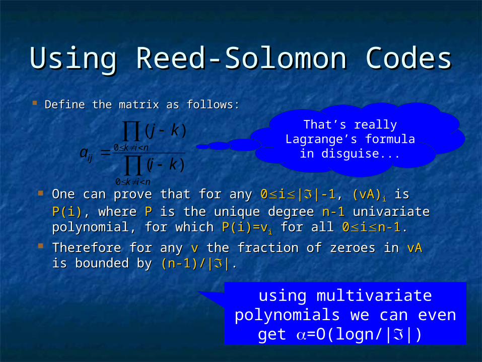
Using Reed-Solomon Codes Using Reed-Solomon Codes Define the matrix as follows:Define the matrix as follows:
nik
nikij ki
kja
0
0
)(
)(
using multivariate polynomials we can even
get =O(logn/||)
That’s really Lagrange’s formula
in disguise...
One can prove that for any One can prove that for any 00ii|||-1|-1, , (vA)(vA)ii is is P(i)P(i), , where where PP is the unique degree is the unique degree n-1n-1 univariate univariate polynomial, for which polynomial, for which P(i)=vP(i)=vii for all for all 00iin-1n-1..
Therefore for any Therefore for any vv the fraction of zeroes in the fraction of zeroes in vAvA is is bounded by bounded by (n-1)/|(n-1)/|||..
2020
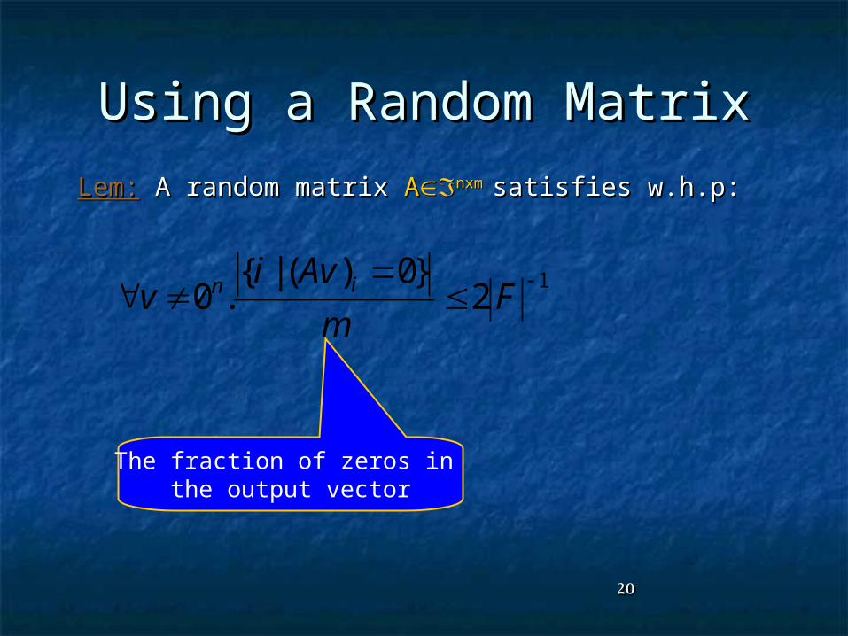
Using a Random MatrixUsing a Random Matrix
Lem:Lem: A random matrix A random matrix AAnxm nxm satisfies w.h.p:satisfies w.h.p:
The fraction of zeros in the output vector
12
}0)(|{.0
Fm
Aviv in
2121
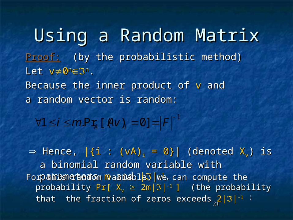
Using a Random MatrixUsing a Random MatrixProof:Proof: (by the probabilistic method) (by the probabilistic method)
Let Let vv00nnnn. .
Because the inner product of Because the inner product of vv and and
a random vector is random:a random vector is random:
1]0)[(Pr.1
FAvmi iA
Hence, Hence, |{i : (vA)|{i : (vA)ii = 0}| = 0}| (denoted (denoted XXvv) is a ) is a binomial random variable with parameters binomial random variable with parameters mm and and ||||-1-1..For this random variable, we can compute the For this random variable, we can compute the
probability probability Pr[ XPr[ Xvv 2m| 2m|||-1 -1 ] ] (the probability that (the probability that the fraction of zeros exceedsthe fraction of zeros exceeds 2| 2|||-1 -1 ))

2222
Using a Random MatrixUsing a Random Matrix
The Chernoff bound:The Chernoff bound:
For a binomial random variable with parameters For a binomial random variable with parameters mm and and ||||-1-1::
1
2
|F|4
mδ
1v 2eδ||X
m
1Pr
F
Hence:Hence:
1|F|4
m
1v 2e||2XPr
Fm
2323
Using a Random MatrixUsing a Random Matrix
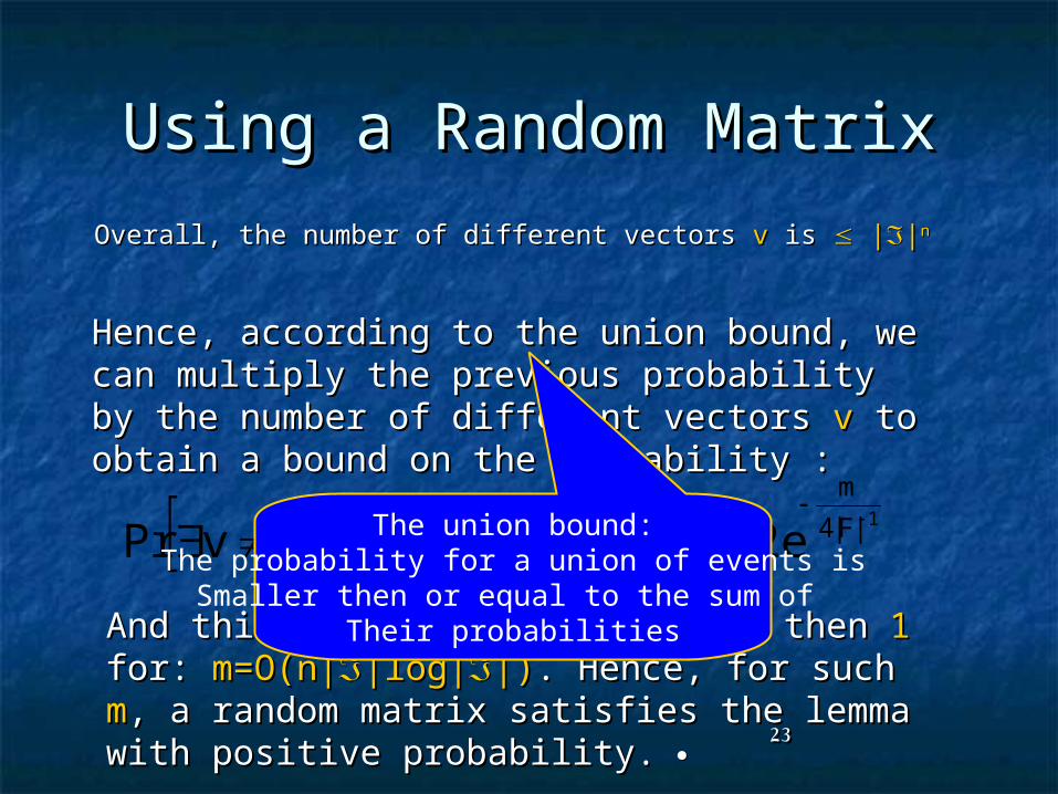
Overall, the number of different vectors Overall, the number of different vectors vv is is | |||nn
Hence, according to the union bound, we can Hence, according to the union bound, we can multiply the previous probability by the multiply the previous probability by the number of different vectors number of different vectors vv to obtain a bound to obtain a bound on the probability :on the probability :
1|F|4
m
11v
n 2e||||2.X0vPr
FFm
And this probability is smaller then And this probability is smaller then 11 for: for: m=O(n|m=O(n||log||log||)|). Hence, for such . Hence, for such mm, a random , a random matrix satisfies the lemma with positive matrix satisfies the lemma with positive probability. probability.
The union bound:The probability for a union of events isSmaller then or equal to the sum of
Their probabilities
2424
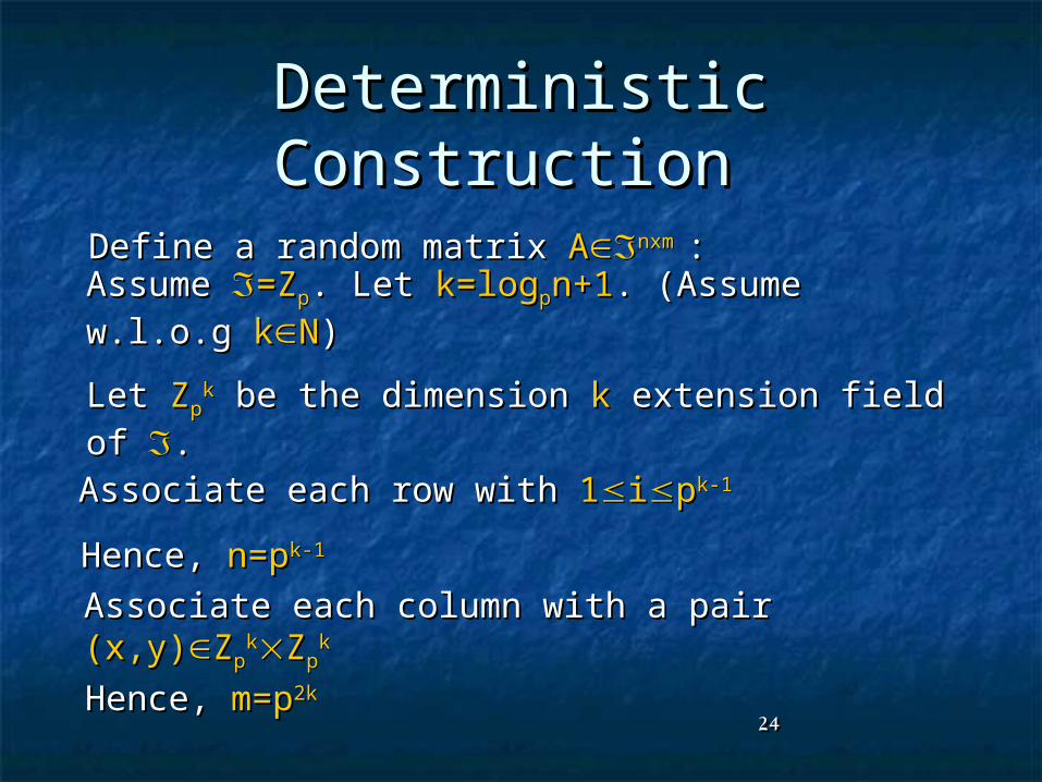
Deterministic Construction Deterministic Construction
Define a random matrix Define a random matrix AAnxm nxm ::
Assume Assume =Z=Zpp. Let . Let k=logk=logppn+1n+1. (Assume w.l.o.g . (Assume w.l.o.g kkNN))
Let Let ZZppkk be the dimension be the dimension kk extension field of extension field of ..
Associate each row with Associate each row with 11iippk-1k-1
Hence, Hence, n=pn=pk-1k-1
Associate each column with a pair Associate each column with a pair (x,y)(x,y)ZZpp
kkZZppkk
Hence, Hence, m=pm=p2k2k

2525
Deterministic Construction Deterministic Construction
pk-1
p2k
<xi,y>
And define And define A(i,(x,y))=A(i,(x,y))= <x<xii,y>,y> (inner (inner product)product)

2626
AnalysisAnalysis For any vector For any vector vvnn, for any column , for any column (x,y)(x,y)ZZpp
kkZZppkk,,
1k1k p
1i
ii
p
1i
iiy)(x, y,xvy,xv(vA)
p2
p
p)p(ppp2k
1k1kkk1k
And thus the fraction of zeroes And thus the fraction of zeroes
The number of zeroes in The number of zeroes in vAvA where where vv00nn
x,y: G(x)=0x,y: G(x)0 <G(x),y>=0
k1k pp 1k1kk p)p(p +
2727
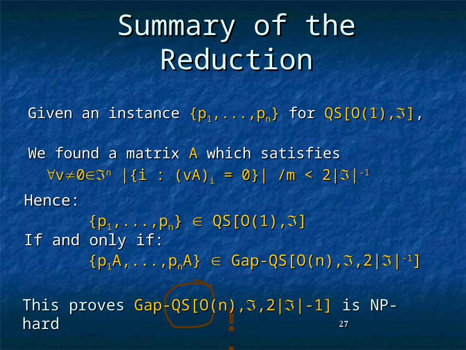
Summary of the ReductionSummary of the Reduction
Given an instance Given an instance {p{p11,...,p,...,pnn}} for for QS[O(1),QS[O(1),]],,
We found a matrix We found a matrix AA which satisfies which satisfies
vv00nn |{i : (vA)|{i : (vA)ii = 0}| /m < 2| = 0}| /m < 2|||-1-1
!!
Hence:Hence:{p{p11,...,p,...,pnn} } QS[O(1), QS[O(1),] ]
If and only if:If and only if: {p{p11A,...,pA,...,pnnA} A} Gap-QS[O(n), Gap-QS[O(n),,2|,2|||-1-1]]
This proves This proves Gap-QS[O(n),Gap-QS[O(n),,2|,2||-1]|-1] is NP-hardis NP-hard
2828
Hitting the RoadHitting the Road
This proves a This proves a PCPPCP characterization with characterization with D=O(n)D=O(n) (hardly (hardly a “local” test...).a “local” test...).
Eventually we’ll prove a characterization with Eventually we’ll prove a characterization with D=O(1)D=O(1) (([DFKRS][DFKRS]) using the results presented here as our ) using the results presented here as our starting point.starting point.