Embed Size (px)
Citation preview
1
Space-time duality in multiple antenna channelsMassimo Franceschetti, Kaushik Chakraborty
Abstract
The concept of information transmission in a multiple antenna channel with scattering objects is stud-
ied from first physical principles. The amount of information that can be transported by electromagnetic
radiation is related to the space-wavenumber and the time-frequency spectra of the system composed by
the transmitting antennas and the scattering objects. The spatial information content is quantified in a
similar fashion than its temporal counterpart, by reducing the inverse problem of field reconstruction to a
communication problem in space, and determining the relevant communication modes of the channel by
rigorously applying the sampling theorem on the field’s vector space. One consequence for narrow-band
frequency transmission is that space and time can be decoupled, leading to a space-time information
duality principle in the computation of the capacity of the radiating system. Interestingly, in the case of
wide-band frequency transmission, it is shown that time and space cannot be decoupled and they jointly
characterize the wave’s information content.
I. INTRODUCTION
The basic consideration that is the leitmotiv of this paper can be stated as follows: in propagation of
electromagnetic (EM) waves, space and frequency are separate but intimately linked objects that pose
fundamental limits on the amount of information carried by scattered fields. Resolving the amount of
information that can be communicated through EM radiation is a venerable subject that has been treated by
a great number of authors in different fields, often leading to rediscovering of basic facts time and again.
Our attempt here is to present a unified approach based on the physical notions of space-wavenumber
and time-frequency spectra of the propagating field.
We consider information sent in the form of waves, hence as a physical process: waves propagate in
space through line of sight, reflection, scattering, and diffraction. Like any other physical phenomenon,
this is governed by the laws of nature. These laws determine not only the process itself, but also the
Research supported in part by the National Science Foundation CAREER award CNS-0546235 and by the California Institute
of Telecommunication and Information Technologies (CALIT2).
The authors are with the California Institute for Telecommunications and Information Technology, Department of Electrical
and Computer Engineering, University of California at San Diego, La Jolla, CA 92037, email: [email protected],
August 23, 2007 DRAFT
amount of diversity that a wave carries along its path. One kind of diversity is due to the wave being
a function of time, hence being characterized by a frequency spectrum. Another kind of diversity is due
to the wave propagating through space. In this case the wave interacts with the propagation environment
and this interaction introduces spatial diversity that can be characterized in terms of spatial bandwidth.
Both kinds of diversities influence the amount of information that can be communicated through wave
propagation. The number of channels available for communication and the amount of information that
can be transported over these channels depend on both the spatial and the frequency bandwidth of the
radiating system.
This paper starts by considering the spatial bandwidth of a radiating system and its information content,
and then considers the interaction between spatial and frequency bandwidths in terms of information
capacity. The broad conclusions that can be drawn from our analysis are as follows. Space can be viewed
as a capacity bearing object: the amount of information communicated by a scattering system increases
with its size and with the size of the receiving antenna array. This is shown rigorously from physics, by
applying the sampling theorem in the space domain. Furthermore, it turns out that in the narrow-band
frequency case, time and space can be decoupled, and the information rate measured in bits per unit time
and summed over all spatial information channels available for transmission, is equivalent to measuring
information rate in bits per unit space and summing over all frequency information channels available for
transmission, thus establishing a space-time information duality principle. On the other hand, in the case
of wide-band frequency transmission, time and space are strongly coupled and they jointly characterize
the information content of the radiating system.
Next, we wish to spend few words on the organization of the paper. Our analysis starts with a
preliminary section where we identify the physical diversity limits of (frequency narrow-band) scat-
tered fields, that were first introduced by Bucci and Franceschetti in the late nineteen eighties [2], [3],
using a functional analysis approach. We then cast these results in a communication theoretic setting,
viewing the inverse problem of field reconstruction through sampling interpolation as a communication
problem. This provides the link between the notion of degrees of freedom of scattered fields and the
corresponding information theoretic definition. That is, between the minimum number of independent
parameters sufficient to completely reconstruct the radiated EM field up to arbitrary precision ε, and
the number of eigenvalues of the MIMO operator (scattering matrix) that are above an arbitrary level
ε. This link was recently pointed out by Migliore [11]. Following these preliminaries, in Section 3 we
present a geometric corollary to Bucci and Franceschetti’s work to determine the relationship between
the minimum non-redundant antenna spacing at the receiver, the wavelength, and the angular aperture of
2
the radiating system and we relate this corollary to to the works of Poon et. al. [15] and Miller [13]. In
Section IV, we examine the spatial information content of the scattered field in more detail, deriving a
purely spatial additive white gaussian noise (AWGN) channel and its corresponding space-time version,
and we point out an information duality principle between space and time, arising from the analysis of
such channels. In Section V we extend the treatment to frequency wide-band transmission, showing the
mutual interaction of space and time in the resolution of the information content of the propagating wave.
Finally, in Section VI, we draw conclusions and outline directions for future work. Throughout the paper,
we point out the practical implications of our analysis and we provide few illustrative examples.
II. PRELIMINARIES
A. Physics background: Bucci-Franceschetti diversity limits
Any real measurement system is invariably affected by a degree of uncertainty. This can stem from
several factors, e.g., background noise, sensitivity and precision of the measuring system, dynamics of
the measurement apparatus, and errors due to numerical approximation. Hence, it is both reasonable and
necessary to consider two electromagnetic field vectors E1 and E2 indistinguishable if their difference,
in a given norm, is below resolution ε, that is
||E1 − E2|| < ε. (1)
Let us now consider a scattering system consisting of an arbitrary number of transmitters (sources)
and scatterers, which are enclosed within a ball B of finite radius a. The receivers are located on an
observation domain lying on an analytical manifold M, which is assumed to be some wavelengths away
from B. For the case of a one-dimensional (open) observation domain, M is an arc spanning the range
[−S, S] in an arbitrary curvilinear coordinate system s. The arclength is normalized with respect to rm,
which is the minimum distance of M from the center of B. All results described here are valid for
one-dimensional observation domains and two-dimensional radiating system, but can be easily extended
to higher dimensions. A schematic diagram of the scattering model is depicted in Figure 1. The primary
sources are assumed to be uniformly bounded, so that the current density (including the polarization
currents) induced on the scatterers satisfies the constraint∫
B|J(r′)| dr′ ≤ η, (2)
where η is a constant. In this section we shall consider narrowband sources, i.e., J(r′) consists of two
impulses in the (temporal) spectral domain at angular frequencies ω and −ω.
3
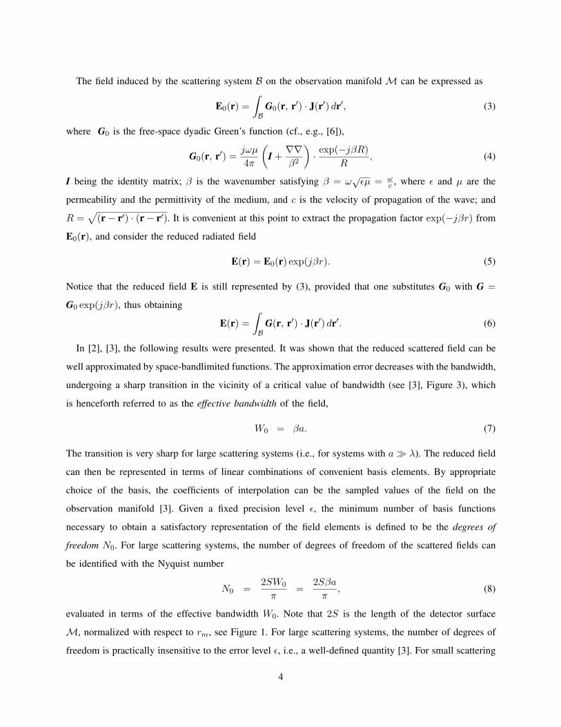
The field induced by the scattering system B on the observation manifold M can be expressed as
E0(r) =∫
BG0(r, r′) · J(r′) dr′, (3)
where G0 is the free-space dyadic Green’s function (cf., e.g., [6]),
G0(r, r′) =jωµ
4π
(I +
∇∇β2
)· exp(−jβR)
R, (4)
I being the identity matrix; β is the wavenumber satisfying β = ω√
εµ = ωc , where ε and µ are the
permeability and the permittivity of the medium, and c is the velocity of propagation of the wave; and
R =√
(r− r′) · (r− r′). It is convenient at this point to extract the propagation factor exp(−jβr) from
E0(r), and consider the reduced radiated field
E(r) = E0(r) exp(jβr). (5)
Notice that the reduced field E is still represented by (3), provided that one substitutes G0 with G =
G0 exp(jβr), thus obtaining
E(r) =∫
BG(r, r′) · J(r′) dr′. (6)
In [2], [3], the following results were presented. It was shown that the reduced scattered field can be
well approximated by space-bandlimited functions. The approximation error decreases with the bandwidth,
undergoing a sharp transition in the vicinity of a critical value of bandwidth (see [3], Figure 3), which
is henceforth referred to as the effective bandwidth of the field,
W0 = βa. (7)
The transition is very sharp for large scattering systems (i.e., for systems with a À λ). The reduced field
can then be represented in terms of linear combinations of convenient basis elements. By appropriate
choice of the basis, the coefficients of interpolation can be the sampled values of the field on the
observation manifold [3]. Given a fixed precision level ε, the minimum number of basis functions
necessary to obtain a satisfactory representation of the field elements is defined to be the degrees of
freedom N0. For large scattering systems, the number of degrees of freedom of the scattered fields can
be identified with the Nyquist number
N0 =2SW0
π=
2Sβa
π, (8)
evaluated in terms of the effective bandwidth W0. Note that 2S is the length of the detector surface
M, normalized with respect to rm, see Figure 1. For large scattering systems, the number of degrees of
freedom is practically insensitive to the error level ε, i.e., a well-defined quantity [3]. For small scattering
4
systems, the dependence of the degrees of freedom on the error level ε was investigated numerically
in [22], but this case is not considered here.
In the examples below, we consider some practical scenarios and illustrate sample values of the spatial
bandwidth and of the number of degrees of freedom for various operating frequencies. Notice that the
spatial bandwidth W0 is normalized to the wavelength λ and hence is a pure number. We shall come
back to these examples several times throughout the paper.
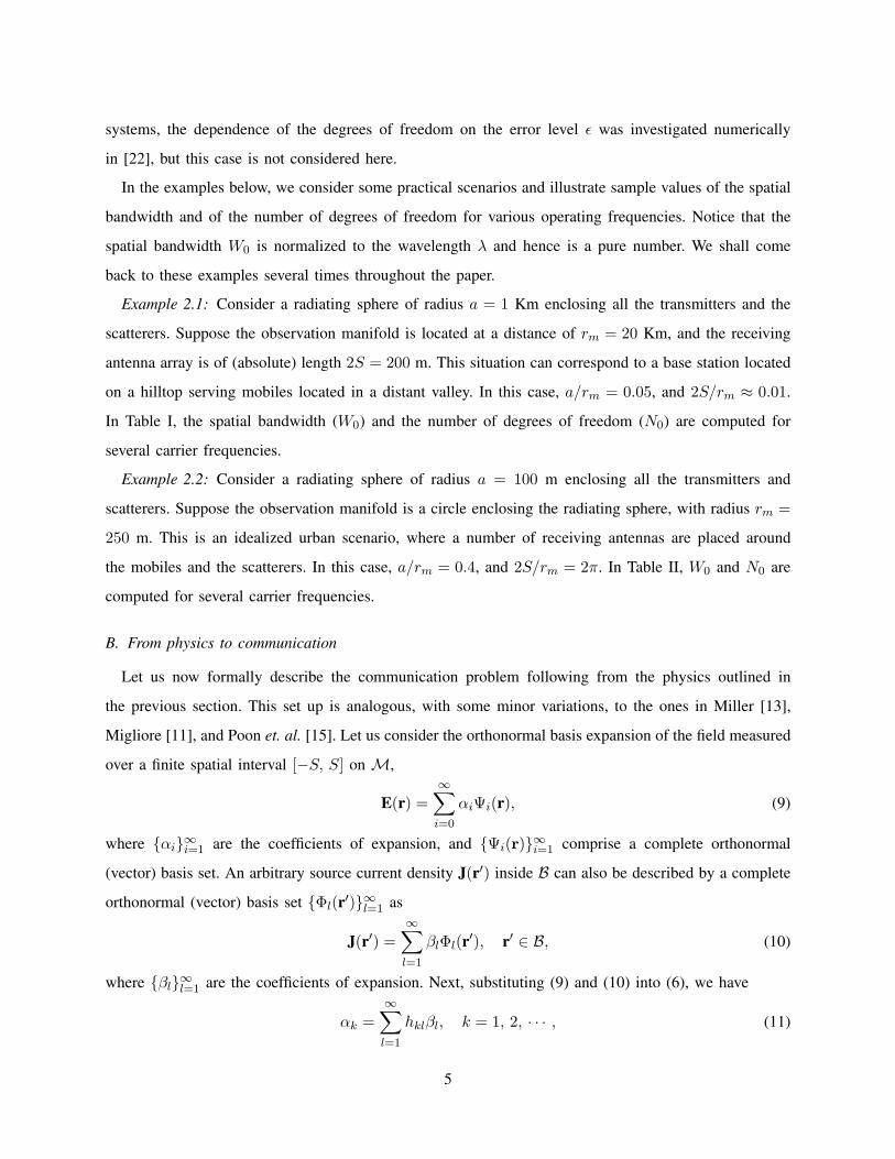
Example 2.1: Consider a radiating sphere of radius a = 1 Km enclosing all the transmitters and the
scatterers. Suppose the observation manifold is located at a distance of rm = 20 Km, and the receiving
antenna array is of (absolute) length 2S = 200 m. This situation can correspond to a base station located
on a hilltop serving mobiles located in a distant valley. In this case, a/rm = 0.05, and 2S/rm ≈ 0.01.
In Table I, the spatial bandwidth (W0) and the number of degrees of freedom (N0) are computed for
several carrier frequencies.
Example 2.2: Consider a radiating sphere of radius a = 100 m enclosing all the transmitters and
scatterers. Suppose the observation manifold is a circle enclosing the radiating sphere, with radius rm =
250 m. This is an idealized urban scenario, where a number of receiving antennas are placed around
the mobiles and the scatterers. In this case, a/rm = 0.4, and 2S/rm = 2π. In Table II, W0 and N0 are
computed for several carrier frequencies.
B. From physics to communication
Let us now formally describe the communication problem following from the physics outlined in
the previous section. This set up is analogous, with some minor variations, to the ones in Miller [13],
Migliore [11], and Poon et. al. [15]. Let us consider the orthonormal basis expansion of the field measured
over a finite spatial interval [−S, S] on M,
E(r) =∞∑
i=0
αiΨi(r), (9)
where αi∞i=1 are the coefficients of expansion, and Ψi(r)∞i=1 comprise a complete orthonormal
(vector) basis set. An arbitrary source current density J(r′) inside B can also be described by a complete
orthonormal (vector) basis set Φl(r′)∞l=1 as
J(r′) =∞∑
l=1
βlΦl(r′), r′ ∈ B, (10)
where βl∞l=1 are the coefficients of expansion. Next, substituting (9) and (10) into (6), we have
αk =∞∑
l=1
hklβl, k = 1, 2, · · · , (11)
5
where hkl =∫M
∫B Ψ∗
k(r) · G(r, r′) · Φl(r′) drdr′. The components hkl can be thought as the coupling
coefficients between the transmission mode l in the ball B and the reception mode k in the manifold M.
In matrix form, (11) is equivalent to
α = H · β, (12)
where α = αk∞k=1 and β = βl∞l=1 are the vectors of coefficients and the elements of the matrix
H are the components hkl. The matrix H can be viewed as the communication operator (viz. the
scattering matrix) between the radiating ball and the receiving manifold. The parameter R = rank(H)
defines the number of degrees of freedom of the communication system, as it determines the number of
parallel independent communication modes. For large scattering systems, recall that the number of basis
functions Ψk required to represent the received field intensity within a given precision tends to N0, the
number of degrees of freedom of the scattered field. Therefore, the linear subspace spanning the rows
of H is at most of dimension N0, so that R ≤ N0. This is the main observation of [11]. Note that the
sources and the scatterers also play an important role in the determination of the exact value of R, since
the rank of H is also dependent on the size of the linear subspace spanned by the columns of H, which
is dictated by the number of orthonormal basis functions φl required to represent the source current
density. In other words, the EM degrees of freedom represent an upper bound on the degrees of freedom
of the MIMO communication channel obtained by considering all possible configurations of sources and
scatterers that can occur inside the radiating ball.
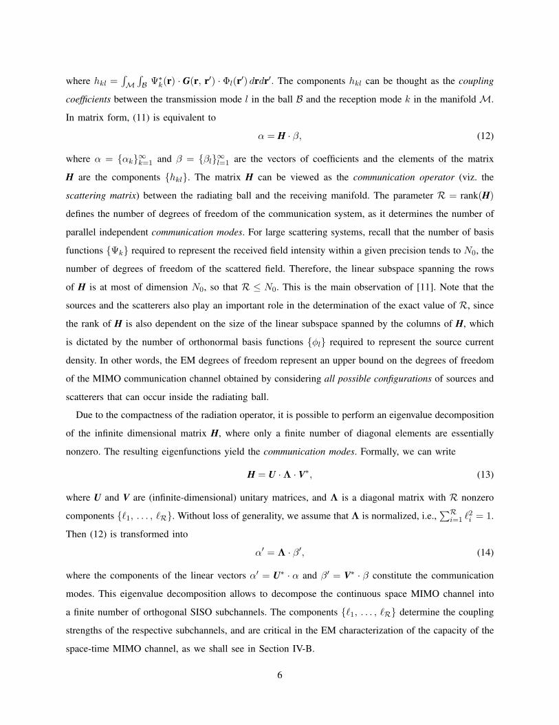
Due to the compactness of the radiation operator, it is possible to perform an eigenvalue decomposition
of the infinite dimensional matrix H, where only a finite number of diagonal elements are essentially
nonzero. The resulting eigenfunctions yield the communication modes. Formally, we can write
H = U ·Λ · V∗, (13)
where U and V are (infinite-dimensional) unitary matrices, and Λ is a diagonal matrix with R nonzero
components `1, . . . , `R. Without loss of generality, we assume that Λ is normalized, i.e.,∑R
i=1 `2i = 1.
Then (12) is transformed into
α′ = Λ · β′, (14)
where the components of the linear vectors α′ = U∗ · α and β′ = V∗ · β constitute the communication
modes. This eigenvalue decomposition allows to decompose the continuous space MIMO channel into
a finite number of orthogonal SISO subchannels. The components `1, . . . , `R determine the coupling
strengths of the respective subchannels, and are critical in the EM characterization of the capacity of the
space-time MIMO channel, as we shall see in Section IV-B.
6
III. MINIMUM NON REDUNDANT ANTENNA SPACING
We now derive a geometric corollary to Bucci and Franceschetti’s work which provides an elegant
interpretation of the number of degrees of freedom, and leads to the determination of the minimum non-
redundant antennas spacing in terms of wavelength and angular aperture of the system. We explicitly
note that this minimum spacing is not heuristic, but it follows directly from physics and from application
of the sampling theorem in the space domain, in light of the considerations made in the previous section.
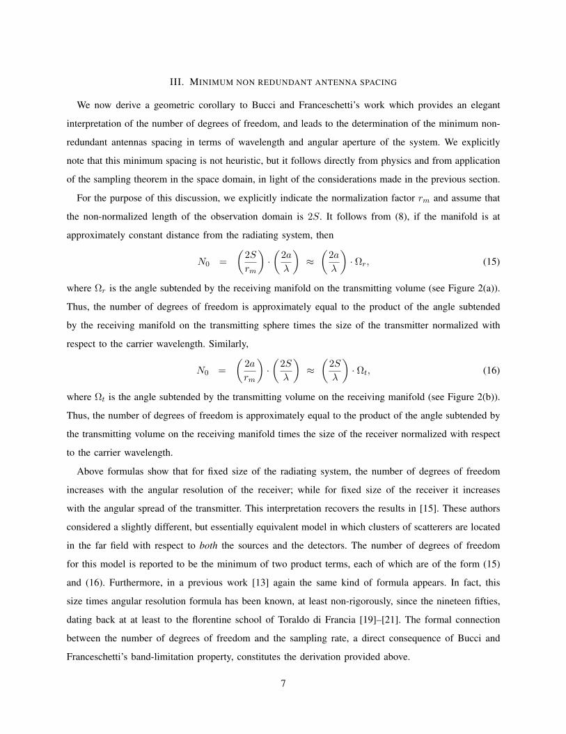
For the purpose of this discussion, we explicitly indicate the normalization factor rm and assume that
the non-normalized length of the observation domain is 2S. It follows from (8), if the manifold is at
approximately constant distance from the radiating system, then
N0 =(
2S
rm
)·(
2a
λ
)≈
(2a
λ
)· Ωr, (15)
where Ωr is the angle subtended by the receiving manifold on the transmitting volume (see Figure 2(a)).
Thus, the number of degrees of freedom is approximately equal to the product of the angle subtended
by the receiving manifold on the transmitting sphere times the size of the transmitter normalized with
respect to the carrier wavelength. Similarly,
N0 =(
2a
rm
)·(
2S
λ
)≈
(2S
λ
)· Ωt, (16)
where Ωt is the angle subtended by the transmitting volume on the receiving manifold (see Figure 2(b)).
Thus, the number of degrees of freedom is approximately equal to the product of the angle subtended by
the transmitting volume on the receiving manifold times the size of the receiver normalized with respect
to the carrier wavelength.
Above formulas show that for fixed size of the radiating system, the number of degrees of freedom
increases with the angular resolution of the receiver; while for fixed size of the receiver it increases
with the angular spread of the transmitter. This interpretation recovers the results in [15]. These authors
considered a slightly different, but essentially equivalent model in which clusters of scatterers are located
in the far field with respect to both the sources and the detectors. The number of degrees of freedom
for this model is reported to be the minimum of two product terms, each of which are of the form (15)
and (16). Furthermore, in a previous work [13] again the same kind of formula appears. In fact, this
size times angular resolution formula has been known, at least non-rigorously, since the nineteen fifties,
dating back at at least to the florentine school of Toraldo di Francia [19]–[21]. The formal connection
between the number of degrees of freedom and the sampling rate, a direct consequence of Bucci and
Franceschetti’s band-limitation property, constitutes the derivation provided above.
7
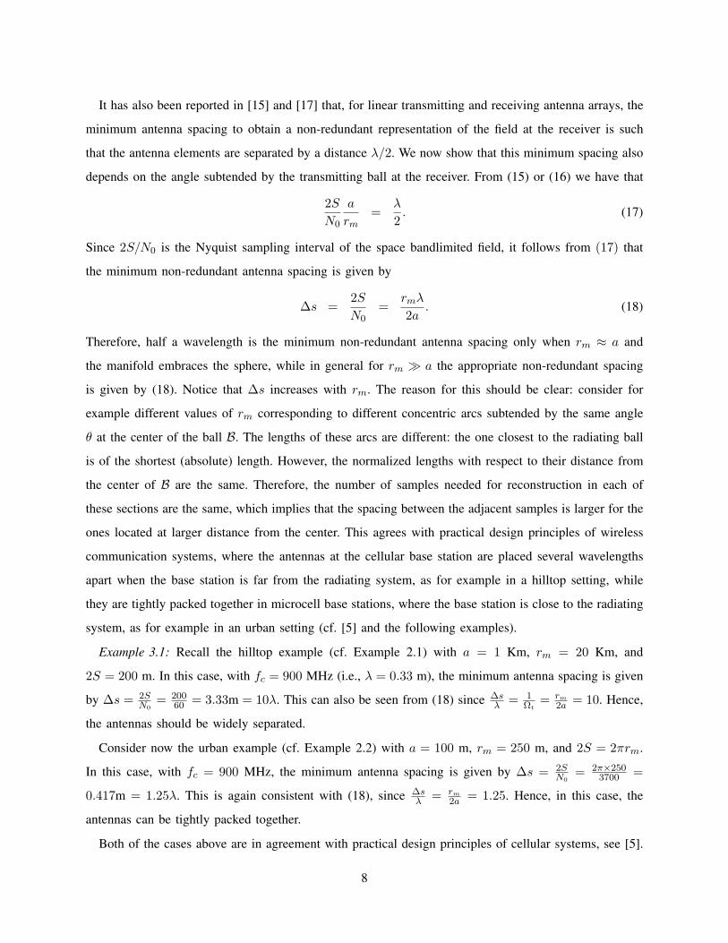
It has also been reported in [15] and [17] that, for linear transmitting and receiving antenna arrays, the
minimum antenna spacing to obtain a non-redundant representation of the field at the receiver is such
that the antenna elements are separated by a distance λ/2. We now show that this minimum spacing also
depends on the angle subtended by the transmitting ball at the receiver. From (15) or (16) we have that
2S
N0
a
rm=
λ
2. (17)
Since 2S/N0 is the Nyquist sampling interval of the space bandlimited field, it follows from (17) that
the minimum non-redundant antenna spacing is given by
∆s =2S
N0=
rmλ
2a. (18)
Therefore, half a wavelength is the minimum non-redundant antenna spacing only when rm ≈ a and
the manifold embraces the sphere, while in general for rm À a the appropriate non-redundant spacing
is given by (18). Notice that ∆s increases with rm. The reason for this should be clear: consider for
example different values of rm corresponding to different concentric arcs subtended by the same angle
θ at the center of the ball B. The lengths of these arcs are different: the one closest to the radiating ball
is of the shortest (absolute) length. However, the normalized lengths with respect to their distance from
the center of B are the same. Therefore, the number of samples needed for reconstruction in each of
these sections are the same, which implies that the spacing between the adjacent samples is larger for the
ones located at larger distance from the center. This agrees with practical design principles of wireless
communication systems, where the antennas at the cellular base station are placed several wavelengths
apart when the base station is far from the radiating system, as for example in a hilltop setting, while
they are tightly packed together in microcell base stations, where the base station is close to the radiating
system, as for example in an urban setting (cf. [5] and the following examples).
Example 3.1: Recall the hilltop example (cf. Example 2.1) with a = 1 Km, rm = 20 Km, and
2S = 200 m. In this case, with fc = 900 MHz (i.e., λ = 0.33 m), the minimum antenna spacing is given
by ∆s = 2SN0
= 20060 = 3.33m = 10λ. This can also be seen from (18) since ∆s
λ = 1Ωt
= rm
2a = 10. Hence,
the antennas should be widely separated.
Consider now the urban example (cf. Example 2.2) with a = 100 m, rm = 250 m, and 2S = 2πrm.
In this case, with fc = 900 MHz, the minimum antenna spacing is given by ∆s = 2SN0
= 2π×2503700 =
0.417m = 1.25λ. This is again consistent with (18), since ∆sλ = rm
2a = 1.25. Hence, in this case, the
antennas can be tightly packed together.
Both of the cases above are in agreement with practical design principles of cellular systems, see [5].
8
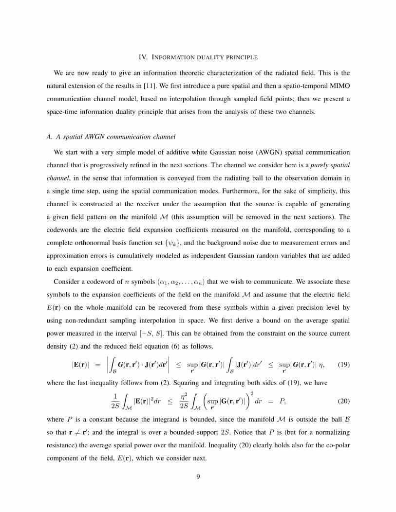
IV. INFORMATION DUALITY PRINCIPLE
We are now ready to give an information theoretic characterization of the radiated field. This is the
natural extension of the results in [11]. We first introduce a pure spatial and then a spatio-temporal MIMO
communication channel model, based on interpolation through sampled field points; then we present a
space-time information duality principle that arises from the analysis of these two channels.
A. A spatial AWGN communication channel
We start with a very simple model of additive white Gaussian noise (AWGN) spatial communication
channel that is progressively refined in the next sections. The channel we consider here is a purely spatial
channel, in the sense that information is conveyed from the radiating ball to the observation domain in
a single time step, using the spatial communication modes. Furthermore, for the sake of simplicity, this
channel is constructed at the receiver under the assumption that the source is capable of generating
a given field pattern on the manifold M (this assumption will be removed in the next sections). The
codewords are the electric field expansion coefficients measured on the manifold, corresponding to a
complete orthonormal basis function set ψk, and the background noise due to measurement errors and
approximation errors is cumulatively modeled as independent Gaussian random variables that are added
to each expansion coefficient.
Consider a codeword of n symbols (α1, α2, . . . , αn) that we wish to communicate. We associate these
symbols to the expansion coefficients of the field on the manifold M and assume that the electric field
E(r) on the whole manifold can be recovered from these symbols within a given precision level by
using non-redundant sampling interpolation in space. We first derive a bound on the average spatial
power measured in the interval [−S, S]. This can be obtained from the constraint on the source current
density (2) and the reduced field equation (6) as follows.
|E(r)| =∣∣∣∣∫
BG(r, r′) · J(r′)dr′
∣∣∣∣ ≤ supr′|G(r, r′)|
∫
B|J(r′)|dr′ ≤ sup
r′|G(r, r′)| η, (19)
where the last inequality follows from (2). Squaring and integrating both sides of (19), we have
12S
∫
M|E(r)|2dr ≤ η2
2S
∫
M
(sup
r′|G(r, r′)|
)2
dr = P, (20)
where P is a constant because the integrand is bounded, since the manifold M is outside the ball Bso that r 6= r′; and the integral is over a bounded support 2S. Notice that P is (but for a normalizing
resistance) the average spatial power over the manifold. Inequality (20) clearly holds also for the co-polar
component of the field, E(r), which we consider next.
9
Assuming an orthornormal basis expansion of the field, by (20) it follows that we have the codeword
constraint1n
n∑
i=1
|αi|2 =1n
∫ S
−S|E(r)|2dr ≤ 2SP
n. (21)
Notice that 2S/n stays constant provided that the sampling rate over the manifold has been fixed and
the spatial codeword length S grows with n.
We now introduce the background noise due to measurement and approximation errors at the receiver.
Let a Gaussian random variable N (0, σ2) be added independently to each transmitted symbol αi, so that
for a transmitted codeword (α1, . . . , αn), the corresponding received codeword (γ1, . . . , γn) is obtained
by
γi = αi + zi, i = 1, . . . , n, (22)
where the zi’s are realizations of i.i.d. N (0, σ2) random variables. We remark here that the index i is a
space index. We can now use Shannon’s formula to state that,
Theorem 1: The information capacity of the spatial additive Gaussian noise channel described above
and subject to the constraint (21) is given by
C =12
log(
1 +P
σ2
)bits per spatial symbol. (23)
It is appropriate at this point to summarize the assumptions we need for above capacity formula to
hold. First of all, we need a non-redundant sampling representation of the field. This ensures that the
coefficients in the codeword, being essentially the same number as the degrees of freedom N0 of the
field, are independent. Since the field is effectively bandlimited [2], this can be ensured by choosing
appropriate basis functions. The second point to notice is that we need the source to be capable of
generating the desired pattern of field coefficients αi on the manifold M. This might not be true in
general and depends on the actual configuration of the sources and the scatterers inside the ball, which
determines the channel communication modes. For example, a portion of the manifold might be shaded
by absorbing obstacles present inside the ball. In this case, the coefficients αi on this portion of the
manifold cannot be excited. In fact, recall from Section II-B that the number of degrees of freedom
of the field measured on the manifold M is an upper bound on the number of degrees of freedom of
the communication system. This upper bound can be achieved considering all possible configurations of
sources and scatterers inside the ball. In the next sections we shall make the dependence on the sources
and the communication modes explicit. Finally, above capacity formula is only valid in the limit of large
10
codeword size, that is as n → ∞. This requires the manifold size to diverge as well, so that 2SP/n
remains constant. In practice, we are constrained to a finite number of observation points placed on a
manifold of finite size. We shall address this last problem in detail at the end of this section.
We now perform one more step to obtain the capacity per unit normalized space over the channel.
This follows by introducing the additional physical constraint of the effective spatial bandwidth W0. This
limits the amount of detectable variation over the manifold of any transmitted signal. By (8), at most
N0 = 2SW0/π different symbols can be transmitted over a spatial region of normalized length 2S. Thus,
the capacity per unit normalized space is given by
C =N0
2S
12
log(
1 +P
σ2
)=
W0
2πlog
(1 +
P
σ2
)bits per normalized length. (24)
The noise is also related to the spatial bandwidth W0. The average power of the (spatial) white Gaussian
noise process is proportional to the spatial bandwidth, so that σ2 = NsWs, where Ws = W02π and Ns is
the constant (spatial) noise power spectral density. Thus, we recover the spatial version of the Shannon-
Hartley formula for communication over a bandlimited channel subject to additive white Gaussian noise,
Theorem 2: The information capacity of the spatial MIMO radiating system depicted in Figure 1,
where transmitters are narrowband with wavelength λ, and the receiving array is subject to additive
white Gaussian noise is given by
C = Ws log(
1 +P
NsWs
)bits per normalized length, (25)
where Ws = W02π = a
λ .
Some observations are now in order. First of all, we note that spatial capacity is measured in bits per
unit of (normalized) space, which correspond to the bits per unit time in the usual temporal formula.
Furthermore, the spatial capacity is associated to an observation interval of (normalized) length 2S;
similarly, the temporal capacity is associated to a time interval of T seconds. In fact, the number of bits
that can be transmitted over the manifold scales with its (normalized) size. In the temporal analogy this
corresponds to the trivial observation that the amount of information transmitted over a time interval
T ′ = 2T corresponds to twice the amount of information sent over a time interval T . In the spatial
domain, the increase is due to a longer receiving array which enhances the angular resolution, i.e., the
detection capability of the receiver. In the temporal domain this corresponds to transmitting more symbols
over the channel using a longer time window. We also note that the spatial capacity scales with the spatial
bandwidth W0 = βa, i.e., with the (wavelength-normalized) size of the radiating system in a same fashion
as the temporal capacity scales with the frequency bandwidth. Since W0 is proportional to the size of the
11
radiating system, this means that a larger radiating system increases the information capacity by working
as a lens enhancing its focusing capability. Furthermore, W0 is inversely proportional to the wavelength,
which means that transmitting at higher frequencies (i.e. shorter wavelengths) can lead, in principle, to
higher information rates.
Next, we turn to the problem that in the usual temporal formulation the capacity formula is derived by
letting T →∞, where T is the time interval of transmission and reception of the continuous function of
time representing the codeword symbols. Instead, in the spatial formulation the normalized spatial interval
is bounded by the total angular spread (2π in the case of a one-dimensional observation domain). This
invariably implies bounded spatial codeword lengths, and hence that the capacity formulas derived above
are not achievable, but rather provide upper bounds on the achievable information rates of the spatial
channel under consideration. We emphasize that this is true even if we stretch the observation domain
to infinity, since the number of degrees of freedom of the electric field induced on the (unbounded)
observation manifold by sources and scatterers enclosed in a bounded volume is still finite, and bounded
by the total angular spread, as it was discussed at the end of Section III.
In this context, it is therefore useful to consider the notion of error exponents arising because the
normalized spatial interval is bounded. The probability of an error event, which occurs when the detected
codeword is different from the transmitted codeword, decays exponentially with n, the number of symbols
in the codeword. The exponent of the error probability indicates the rate of decay of the error event,
and is a useful channel parameter. For the AWGN channel, upper bounds on the error exponent are well
known (cf., e.g., [7], Theorem 7.4.4). In the following example we apply such bounds showing that, with
a larger N0, information rates closer to capacity can be achieved. A large value of N0 can be achieved
by using a higher carrier frequency, and/or by using a large scattering system, and/or by using a large
observation domain size. It should be noted that these estimates are based on the upper bounds on error
probability, and the actual achievable rates can in fact be higher.
Example 4.1: Recall the hilltop example (Example 2.1) with a = 1 Km, rm = 20 Km, and 2S = 200
m, and the urban example (Example 2.2) with a = 100 m, rm = 250 m, and 2S = 2πrm. In Table III,
the ratio of the maximum achievable information rate to the channel capacity (Rmax/C) corresponding
to Pe ≤ 10−6 for SNR = 0 dB are computed for several carrier frequencies for all of these scenarios.
B. A space-time AWGN communication channel
In this section, the source geometry is taken into account so that an explicit relation between input
(represented by the current density inside the ball) and output (represented by the observed EM field on
12
the manifold) is obtained. Furthermore, we consider transmission over both space and time. There has
been a plethora of recent publications that provide a space-time MIMO model based on the physics of
propagation [1], [8]–[13], [15]–[17], [23]. The common denominator of all of these works follows the
outline given in Section II-B, where the MIMO channel is decomposed into a set of R parallel SISO
subchannels, as given by equation (14).
As in the case of the purely spatial channel model, we can introduce the effects of background noise
via a simple AWGN model. From (14) it follows that the measured communication modes are given by
γ′i = α′i + zi = `i β′i + zi, i = 1, · · · , R, (26)
where zi are realizations of i.i.d. N (0, σ2) random variables which are added to each space component
at a given instant of time; `i, i = 1, · · · , R are the nonzero diagonal elements of Λ; and the input
coefficients are subject to a power constraint
1R
R∑
l=1
|β′l |2 ≤ P ′, (27)
where P ′ can be immediately related to η. Recall from Section II-B that R is the number of independent
parallel SISO subchannels, as determined by the singular value decomposition of the channel matrix H;
furthermore, R ≤ N0, where N0 is the number of degrees of freedom of the scattered field, i.e., the
number of orthogonal basis functions required to represent the field within a given precision level.
We now let the R spatial channels defined by equation (26) evolve over time, assuming independent
additive Gaussian noise added at each measurement over time as well. We thus obtain a parallel Gaussian
channel, formed by the R spatial communication modes, whose capacity is well known (cf. [18]) to be
C =R∑
i=1
Wt log(
1 +P ∗
i `2i
WtNt
)bits per unit time, (28)
where Wt is the temporal frequency bandwidth, Nt is the (constant) power spectral density of the
additive white Gaussian noise in the time evolution, WtNt = σ2, and P ∗i are the waterfilling power
allocations [4]. If the communication modes are roughly of the same strength, i.e., `2i ≈ 1
R , then the
space-time capacity expression (28) simplifies to the sum of R identical parallel subchannels, given by
C = RWt log(
1 +P ′
RWtNt
)bits per unit time, (29)
where the waterfilling power allocation allocates equal power P ′ to all channels.
13
C. A space-time information duality principle
Assuming the sources to be able to excite all N0 degrees of freedom of the field, we can perform the
substitution R = N0 = 2Ωraλ = Ws2Ωr, obtaining
C = 2ΩrWsWt log(
1 +P ′
2ΩrWsWtNt
)bits per unit time. (30)
Above formula shows the space-time capacity in bits per unit time when the space-time channel is used
over time and this channel also exploits the space diversity given by N0 = 2ΩrWs spatial degrees of
freedom.
Similarly, we can obtain a dual formula for the space-time capacity in bits per normalized length,
when the space-time channel is used in space as defined by Theorem 2, and this channel also exploits
the time diversity of Wt2T degrees of freedom given by a frequency bandwidth Wt. In this case, we
need to modify (25) to relate the coefficients αi to the communication modes. By assuming as before
all the communication modes to be of the same strength, we let
γ′i = α′i + zi = `β′i + zi,
with `2 = 1Wt2T . The waterfilling power allocations allocate equal power P ′ to all frequency channels
and we have
C = 2TWtWs log(
1 +P ′
2TWtWsNs
)bits per unit length. (31)
By comparing equations (30) and (31), we can now state the following space-time information duality
principle.
Information duality principle. The physical space-time AWGN channel can be operated in time, by
summing all the relevant spatial information channels that are related to the (spatial) degrees of freedom of
the scattered field through application of the sampling theorem in space. In a dual way the same channel
can be operated, in principle, in space (given acceptable error exponents due to the angular resolution
limit), by summing all the relevant frequency information channels that are related to the (temporal)
degrees of freedom of the scattered field through application of the sampling theorem in time.
It follows that there are two equivalent ways of measuring information capacity: in the first case this
is measured in bits per unit time, while in the second case it is measured in bits per units of normalized
space. The two information measures are equivalent representations of the same concept of information
rate through space and time, in a MIMO system, projected along each of these dimensions. Notice that
while the time dimension is present in the first information measure, the second information measure is
14
a pure number. This is because the bandwidth Wt is measured in Hz, while the spatial bandwidth Ws,
being normalized to the wavelength, is a pure number. It follows that the two equations (30) and (31)
cannot be directly compared. However, we can make both representations independent of dimension by
normalizing the bandwidth Wt to the carrier frequency f0 = 1/τ0. In this case we measure (30) in bits
per time normalized to τ0, and (31) in bits per length normalized to λ. A quantitative comparison is now
possible, and we see that the two equations coincide, provided that normalized variables Ωr = 2S/rm
and T/τ0 are equal. This means that in our ideal dual-operation of the space-time channel, the codeword
spatial length corresponding to the observation domain 2S, normalized to rm, must be equal to the
codeword temporal length T , normalized to the period of the temporal carrier frequency τ0.
V. WIDE-BAND FREQUENCY SPECTRUM
The information theoretic characterization of the radiated field presented in the previous section was
based on narrow-band frequency signals. We have assumed that the spatial bandwidth W0 remains constant
over the (narrow) frequency band Wt used for transmission. In this way, the information contents along
the space and time dimensions could be treated independently and led to the information duality principle.
We now want to make a first step in the direction of understanding the properties of the signal received
on the manifold M when the narrow-band assumption is relaxed. In this case, we need to account for
the dependence between the spatial band and the frequency band of the radiated wave, generalizing the
single frequency treatment of Bucci and Franceschetti [2], [3]. As we shall see in the following, this
leads to a variable space-time sampling rate defining the information content of the scattered wave.
Let us start writing the space-time domain representation of the field over the manifold, which is a
real function,
e(t, s) =12π
∫ +∞
−∞dω eiωt
∫ ωa/c
−ωa/cdu e−iusE(ω, u), (32)
where E(ω, u) is the frequency-wavenumber representation of the received signal, s is the curvilinear
coordinate over the manifold, a is the size of the radiating ball, c is the speed of light, and ωa/c = W0
is the spatial bandwidth of the radiating system at angular frequency ω. Note that in (32) the (real)
space-time field representation is obtained by transforming E(ω, u) with respect to the wavenumber and
then inverse transforming with respect to the angular frequency. Letting the inner integral be F(ω, s),
we note that
e(t, s) =12π
∫ +∞
−∞dω eiωtF(ω, s) (33)
15
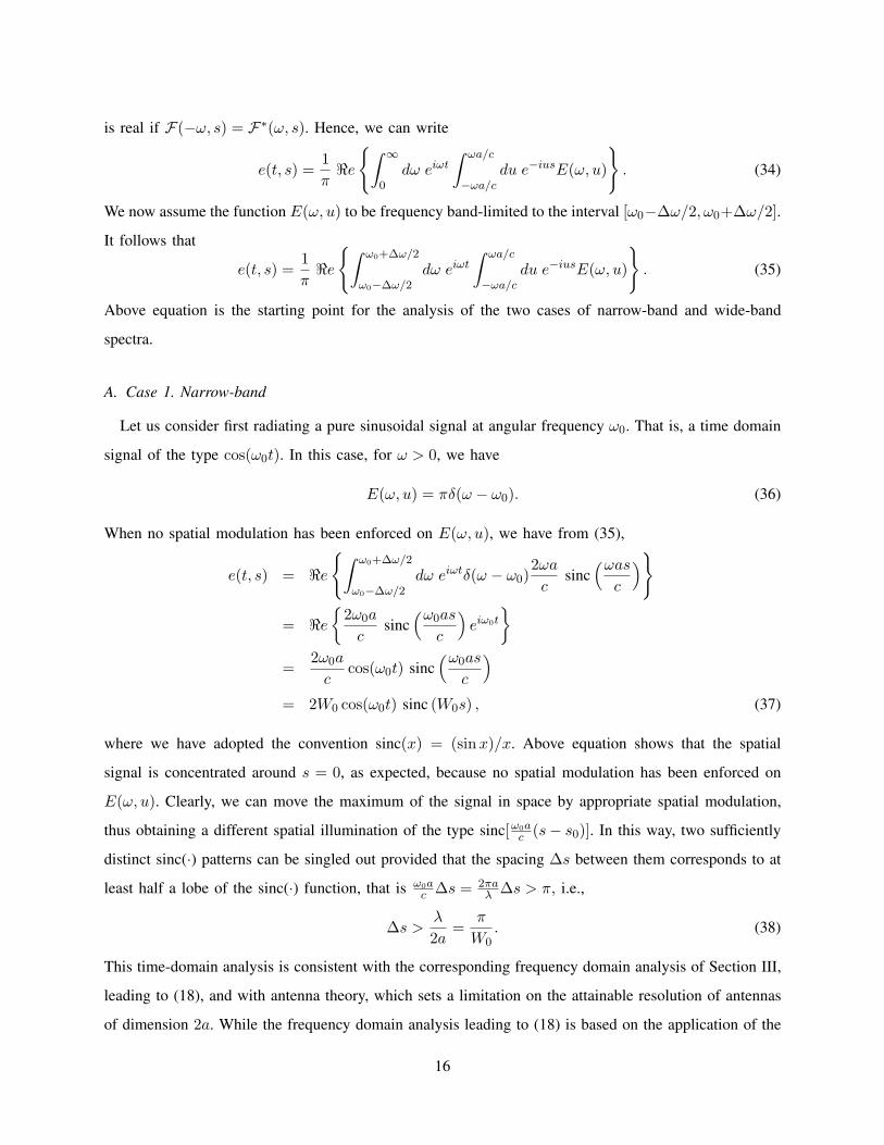
is real if F(−ω, s) = F∗(ω, s). Hence, we can write
e(t, s) =1π<e
∫ ∞
0dω eiωt
∫ ωa/c
−ωa/cdu e−iusE(ω, u)
. (34)
We now assume the function E(ω, u) to be frequency band-limited to the interval [ω0−∆ω/2, ω0+∆ω/2].
It follows that
e(t, s) =1π<e
∫ ω0+∆ω/2
ω0−∆ω/2dω eiωt
∫ ωa/c
−ωa/cdu e−iusE(ω, u)
. (35)
Above equation is the starting point for the analysis of the two cases of narrow-band and wide-band
spectra.
A. Case 1. Narrow-band
Let us consider first radiating a pure sinusoidal signal at angular frequency ω0. That is, a time domain
signal of the type cos(ω0t). In this case, for ω > 0, we have
E(ω, u) = πδ(ω − ω0). (36)
When no spatial modulation has been enforced on E(ω, u), we have from (35),
e(t, s) = <e
∫ ω0+∆ω/2
ω0−∆ω/2dω eiωtδ(ω − ω0)
2ωa
csinc
(ωas
c
)
= <e
2ω0a
csinc
(ω0as
c
)eiω0t
=2ω0a
ccos(ω0t) sinc
(ω0as
c
)
= 2W0 cos(ω0t) sinc (W0s) , (37)
where we have adopted the convention sinc(x) = (sinx)/x. Above equation shows that the spatial
signal is concentrated around s = 0, as expected, because no spatial modulation has been enforced on
E(ω, u). Clearly, we can move the maximum of the signal in space by appropriate spatial modulation,
thus obtaining a different spatial illumination of the type sinc[ω0ac (s− s0)]. In this way, two sufficiently
distinct sinc(·) patterns can be singled out provided that the spacing ∆s between them corresponds to at
least half a lobe of the sinc(·) function, that is ω0ac ∆s = 2πa
λ ∆s > π, i.e.,
∆s >λ
2a=
π
W0. (38)
This time-domain analysis is consistent with the corresponding frequency domain analysis of Section III,
leading to (18), and with antenna theory, which sets a limitation on the attainable resolution of antennas
of dimension 2a. While the frequency domain analysis leading to (18) is based on the application of the
16
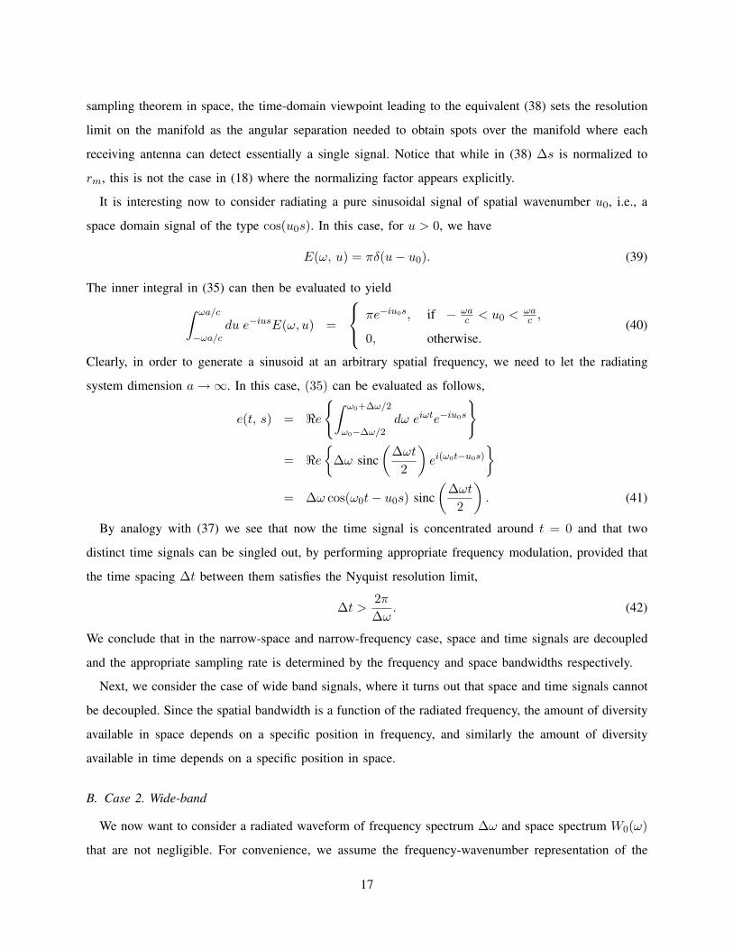
sampling theorem in space, the time-domain viewpoint leading to the equivalent (38) sets the resolution
limit on the manifold as the angular separation needed to obtain spots over the manifold where each
receiving antenna can detect essentially a single signal. Notice that while in (38) ∆s is normalized to
rm, this is not the case in (18) where the normalizing factor appears explicitly.
It is interesting now to consider radiating a pure sinusoidal signal of spatial wavenumber u0, i.e., a
space domain signal of the type cos(u0s). In this case, for u > 0, we have
E(ω, u) = πδ(u− u0). (39)
The inner integral in (35) can then be evaluated to yield∫ ωa/c
−ωa/cdu e−iusE(ω, u) =
πe−iu0s, if − ωac < u0 < ωa
c ,
0, otherwise.(40)
Clearly, in order to generate a sinusoid at an arbitrary spatial frequency, we need to let the radiating
system dimension a →∞. In this case, (35) can be evaluated as follows,
e(t, s) = <e
∫ ω0+∆ω/2
ω0−∆ω/2dω eiωte−iu0s
= <e
∆ω sinc
(∆ωt
2
)ei(ω0t−u0s)
= ∆ω cos(ω0t− u0s) sinc(
∆ωt
2
). (41)
By analogy with (37) we see that now the time signal is concentrated around t = 0 and that two
distinct time signals can be singled out, by performing appropriate frequency modulation, provided that
the time spacing ∆t between them satisfies the Nyquist resolution limit,
∆t >2π
∆ω. (42)
We conclude that in the narrow-space and narrow-frequency case, space and time signals are decoupled
and the appropriate sampling rate is determined by the frequency and space bandwidths respectively.
Next, we consider the case of wide band signals, where it turns out that space and time signals cannot
be decoupled. Since the spatial bandwidth is a function of the radiated frequency, the amount of diversity
available in space depends on a specific position in frequency, and similarly the amount of diversity
available in time depends on a specific position in space.
B. Case 2. Wide-band
We now want to consider a radiated waveform of frequency spectrum ∆ω and space spectrum W0(ω)
that are not negligible. For convenience, we assume the frequency-wavenumber representation of the
17
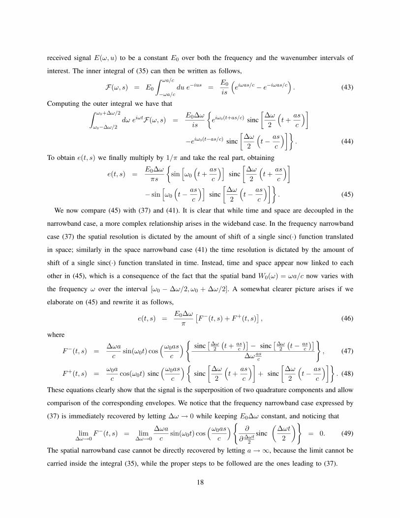
received signal E(ω, u) to be a constant E0 over both the frequency and the wavenumber intervals of
interest. The inner integral of (35) can then be written as follows,
F(ω, s) = E0
∫ ωa/c
−ωa/cdu e−ius =
E0
is
(eiωas/c − e−iωas/c
). (43)
Computing the outer integral we have that∫ ω0+∆ω/2
ω0−∆ω/2dω eiωtF(ω, s) =
E0∆ω
is
eiω0(t+as/c) sinc
[∆ω
2
(t +
as
c
)]
−eiω0(t−as/c) sinc[∆ω
2
(t− as
c
)]. (44)
To obtain e(t, s) we finally multiply by 1/π and take the real part, obtaining
e(t, s) =E0∆ω
πs
sin
[ω0
(t +
as
c
)]sinc
[∆ω
2
(t +
as
c
)]
− sin[ω0
(t− as
c
)]sinc
[∆ω
2
(t− as
c
)]. (45)
We now compare (45) with (37) and (41). It is clear that while time and space are decoupled in the
narrowband case, a more complex relationship arises in the wideband case. In the frequency narrowband
case (37) the spatial resolution is dictated by the amount of shift of a single sinc(·) function translated
in space; similarly in the space narrowband case (41) the time resolution is dictated by the amount of
shift of a single sinc(·) function translated in time. Instead, time and space appear now linked to each
other in (45), which is a consequence of the fact that the spatial band W0(ω) = ωa/c now varies with
the frequency ω over the interval [ω0 − ∆ω/2, ω0 + ∆ω/2]. A somewhat clearer picture arises if we
elaborate on (45) and rewrite it as follows,
e(t, s) =E0∆ω
π
[F−(t, s) + F+(t, s)
], (46)
where
F−(t, s) =∆ωa
csin(ω0t) cos
(ω0as
c
)sinc
[∆ω2
(t + as
c
)]− sinc[
∆ω2
(t− as
c
)]
∆ω asc
, (47)
F+(t, s) =ω0a
ccos(ω0t) sinc
(ω0as
c
) sinc
[∆ω
2
(t +
as
c
)]+ sinc
[∆ω
2
(t− as
c
)]. (48)
These equations clearly show that the signal is the superposition of two quadrature components and allow
comparison of the corresponding envelopes. We notice that the frequency narrowband case expressed by
(37) is immediately recovered by letting ∆ω → 0 while keeping E0∆ω constant, and noticing that
lim∆ω→0
F−(t, s) = lim∆ω→0
∆ωa
csin(ω0t) cos
(ω0as
c
)∂
∂ ∆ωt2
sinc(
∆ωt
2
)= 0. (49)
The spatial narrowband case cannot be directly recovered by letting a →∞, because the limit cannot be
carried inside the integral (35), while the proper steps to be followed are the ones leading to (37).
18
VI. CONCLUSION
In MIMO systems communication is performed through EM waves and the concept of information
transmission is related to the amount of diversity EM waves can carry. Such diversity lies in two different
dimensions: time and space. The classical view of Shannon’s information theory typically considers only
the time dimension along with its transformed counterpart: the frequency spectrum. We have shown that
Shannon’s theory can also be applied to the space dimension which, analogous to time, becomes a capacity
bearing object. The concept of transformed space domain and space bandwidth has been introduced and
an information duality principle has shown that space and time can naturally be treated as the dual of one
another. In the wide-band transmission regime a much more complex scenario arises. In this case, time
and space are linked together, as the space bandwidth depends on the radiated frequency. Our analysis
appears to be open to several refinements. In particular, characterization of the capacity in the frequency
wide-band regime and showing that although space and time are not decoupled, information is conserved
in space-time are interesting open problems.
VII. ACKNOWLEDGEMENT
The authors wish to acknowledge enlightening conversations they had on the subject with Prof. Giorgio
Franceschetti, to whom this work is dedicated.
REFERENCES
[1] T. D. Abhayapala, T. S. Pollock and R. A. Kennedy, “Spatial decomposition of MIMO wireless channels,” in Proc. Seventh
International Symposium on Signal Processing and its Applications, ISSPA 2003, Paris, pp. 309 -312, Vol. 1, July 2003.
[2] O. M. Bucci and G. Franceschetti, “On the spatial bandwidth of scattered fields,” IEEE Trans. Antennas Propagat., 35(12):
1445–1455, Dec 1987.
[3] O. M. Bucci and G. Franceschetti, “On the degrees of freedom of scattered fields,” IEEE Trans. Antennas Propagat., 37(7):
918–926, July 1989.
[4] T. M. Cover and J. A. Thomas, Elements of Information Theory, John Wiley & Sons, New York, 1991.
[5] M. P. Fitz, C. Shen, and M. Samuel, “The wireless communications physical layer,” in G. Franceschetti and S. Stornelli
Eds., Wireless Networks: From the Physical Layer to Communication, Computing, Sensing, and Control, Chapter 2, Elsevier
Inc., 2006.
[6] G. Franceschetti, Electromagnetics: Theory, Techniques, and Engineering Paradigms, Kluwer Academic, 1998.
[7] R. G. Gallager, Information Theory and Reliable Communication, John Wiley & Sons, New York, 1968.
[8] L. W. Hanlen and M. Fu, “Wireless communication systems with spatial diversity: a volumetric approach,” Proceedings of
the ICC 2003, 2673–2677, vol. 4, May 2003.
[9] L. W. Hanlen and M. Fu, “Capacity of MIMO channels: a volumetric approach,” Proceedings of the ICC 2003, 3001–3005,
vol. 5, May 2003.
19
[10] R. A. Kennedy and T. D. Abhayapala, “Spatial concentration of wave-fields: towards spatial information content in arbitrary
multipath scattering,” in Proc. Fourth Australian Communications Theory Workshop, AusCTW2003, pp 3845, Melbourne,
Australia, Feb 5-7, 2003.
[11] M. D. Migliore, “On the role of the number of degrees of freedom of the field in MIMO channels,” IEEE Trans. Antennas
Propagat., 54(2): 620–628, Feb 2006.
[12] M. D. Migliore, “Restoring the symmetry between space domain and time domain in the channel capacity of MIMO
communication systems,” in Proc. 2006 IEEE Antennas & Propagation International Symposium, pp. 333–336, July 2006.
[13] D. A. B. Miller, “Communicating with waves between volumes: evaluating orthogonal spatial channels and limits on
coupling strengths,” Appl. Optics, 39(11): 1681–1699, Apr 2000.
[14] T. S. Pollock, T. D. Abhayapala and R. A. Kennedy, “Spatial Limits to MIMO Capacity in General Scattering Environments,”
in Proc. 7th International Symposium on DSP for Communication Systems (DSPCS03), pp 49-54, Dec 2003.
[15] A. S. Y. Poon, R. W. Brodersen, and D. N. C. Tse, “Degrees of freedom in multiple-antenna channels: a signal space
approach,” IEEE Trans. Inform. Theory, 51(2): 523–536, Feb 2005.
[16] A. S. Y. Poon, R. W. Brodersen, and D. N. C. Tse, “Impact of scattering on the capacity, diversity, and propagation range
of multiple-antenna channels,” IEEE Trans. Inform. Theory, 52(3): 1087–1100, Mar 2006.
[17] A. M. Sayeed, “Deconstructing multiantenna fading channels,” IEEE Trans. Signal Processing, 50(10): 2563–2579, Oct
2002.
[18] I. E. Telatar. “Capacity of multi-antenna Gaussian channels,” European Transactions on Telecommunications, 10(6),
585–595, 1999.
[19] G. Toraldo di Francia, “Resolving power and information,” J. Optical Society America, 45(7): 497–501, July 1955.
[20] G. Toraldo di Francia. “Directivity, super-gain and information,” IRE Trans. Antennas Propagat., AP-4(3): 473–478, July
1956.
[21] G. Toraldo di Francia, “Degrees of freedom of an image,” J. Optical Society America, 59(7): 799–804, July 1969.
[22] J. Xu and R. Janaswamy, “Electromagnetic degrees of freedom in 2-D scattering environments,” IEEE Trans. Antennas
Propagat., vol. 54, no. 12, pp. 3882–3894, Dec. 2006.
[23] J. W. Wallace and M. A. Jensen, “Intrinsic capacity of the MIMO wireless channel,” in Proc. IEEE Vehicular Technology
Conf., vol. 2, pp. 701–705, Vancouver, CA, Sep. 2002.
20
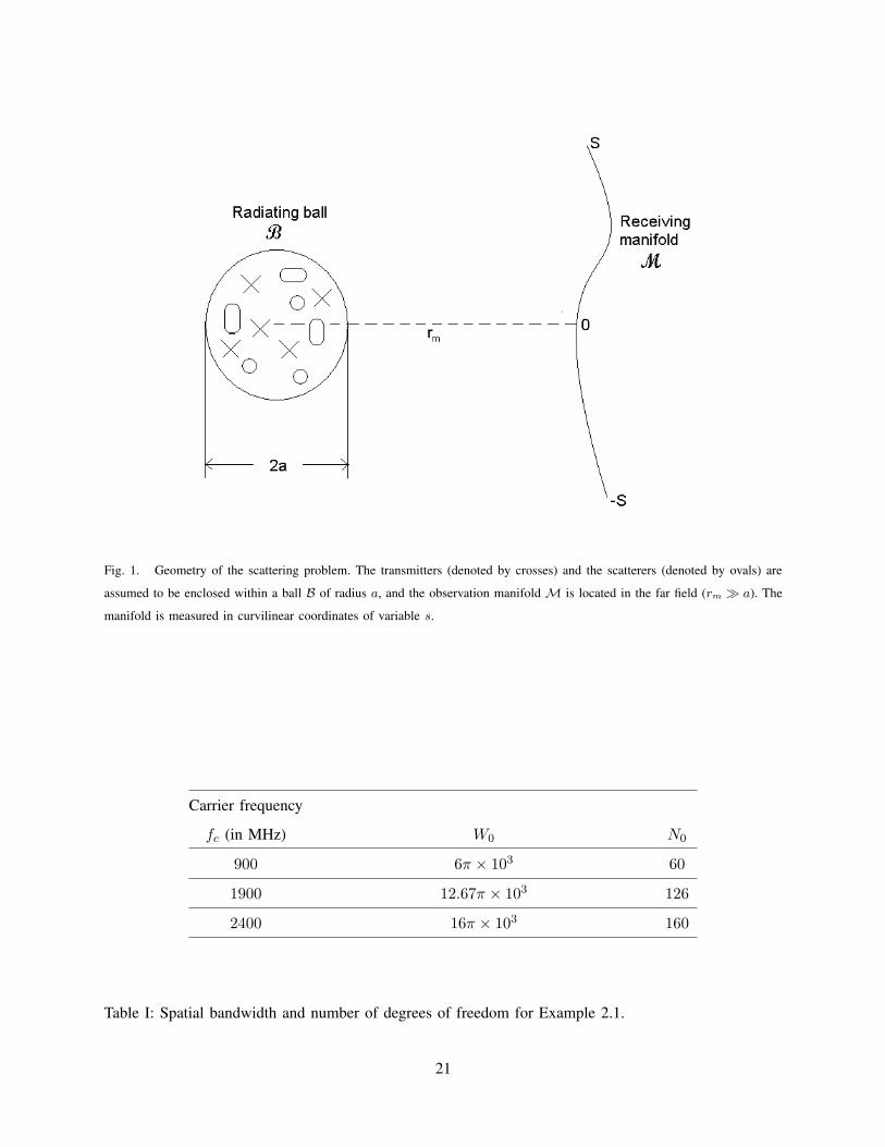
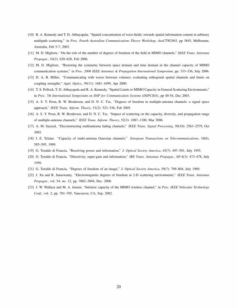
Fig. 1. Geometry of the scattering problem. The transmitters (denoted by crosses) and the scatterers (denoted by ovals) are
assumed to be enclosed within a ball B of radius a, and the observation manifold M is located in the far field (rm À a). The
manifold is measured in curvilinear coordinates of variable s.
Carrier frequency
fc (in MHz) W0 N0
900 6π × 103 60
1900 12.67π × 103 126
2400 16π × 103 160
Table I: Spatial bandwidth and number of degrees of freedom for Example 2.1.
21
2a
0
S
-S
Transmitting ball
B
Receiving manifold
M
Ω r
(a)
2a
0
S
-S
Transmitting ball
B
Receiving manifold
M
Ωt
(b)
Fig. 2. Geometric interpretation of the number of degrees of freedom of the scattered field.
Carrier frequency
fc (in MHz) W0 N0
900 6π × 102 3770
1900 12.67π × 102 7960
2400 16π × 102 10053
Table II: Spatial bandwidth and number of degrees of freedom for Example 2.2.
Carrier frequency Rmax/C
fc (in MHz) Example 2.1 Example 2.2
900 0.01 0.853
1900 0.318 0.9
2400 0.385 0.908
Table III: Table of values for Example 4.1.
22