1

Software Cost Estimation

2

Outline

Introduction

Inputs and Outputs

Methods of Estimation

COCOMO

Conclusion

3

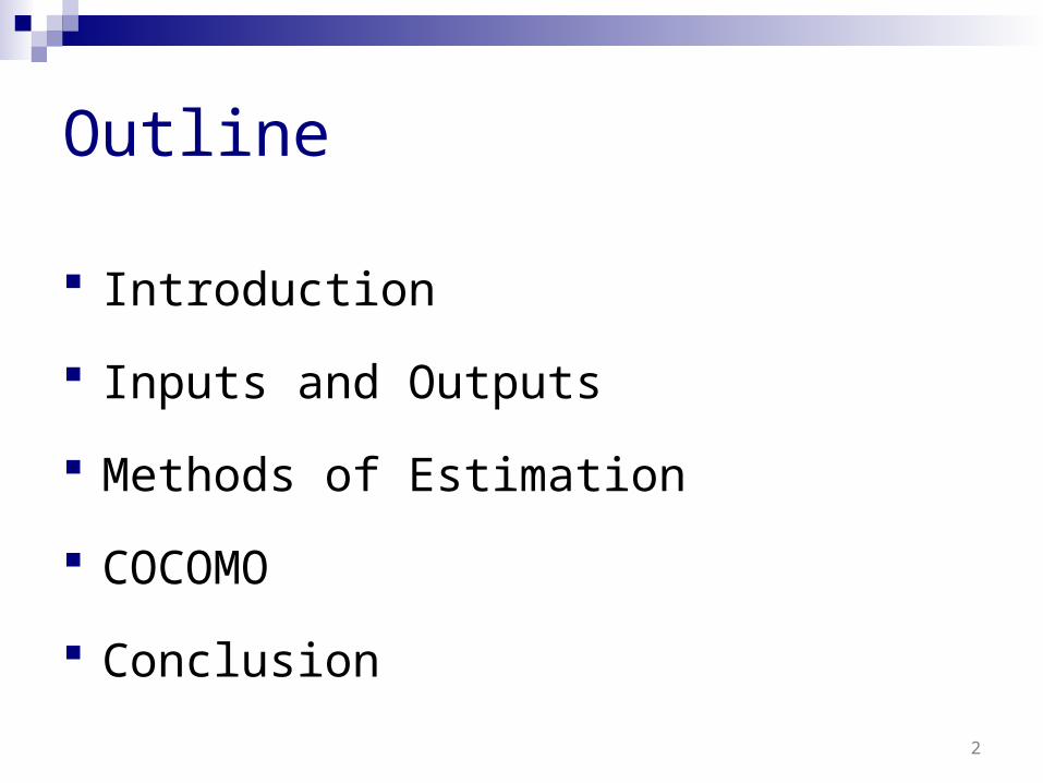
Cost Estimation Is Needed

55% of projects over budget 24 companies that developed large distributed

systems (1994) 53% of projects cost 189% more than

initial estimates Standish Group of 8,380 projects (1994)

4

Cost Estimation An approximate judgment of the costs for a project

Many variables Often measured in terms of effort (i.e., person

months/years) Different development environments will determine

which variables are included in the cost value Management costs Development costs

Training costs Quality assurance

Resources

5

Cost Estimation Affects

Planning and budgeting Requirements prioritization Schedule Resource allocation

Project management Personnel Tasks

6

General Steps and Remarks

Establish Plan What data should we gather Why are we gathering this data What do we hope to accomplish

Do cost estimation for initial requirements Decomposition

Use several methods There is no perfect technique If get wide variances in methods, then should re-evaluate

the information used to make estimates

7

General Steps and Remarks (cont.)

Do re-estimates during life cycle Make any required changes to development Do a final assessment of cost estimation at the

end of the project

8

Software Cost Estimation Process Definition

A set of techniques and procedures that is used to derive the software cost estimate

Set of inputs to the process and then the process will use these inputs to generate the output

9

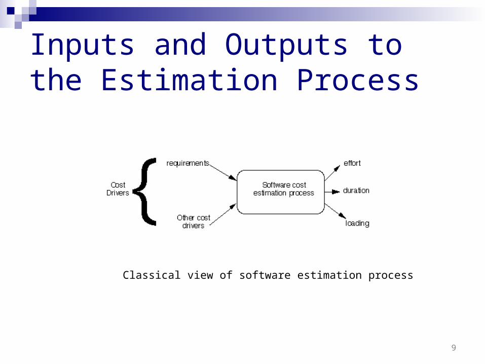
Inputs and Outputs to the Estimation Process

Classical view of software estimation process

10

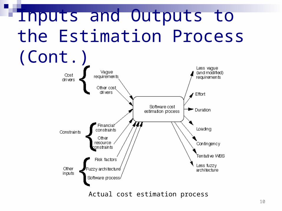
Inputs and Outputs to the Estimation Process (Cont.)

Actual cost estimation process

11

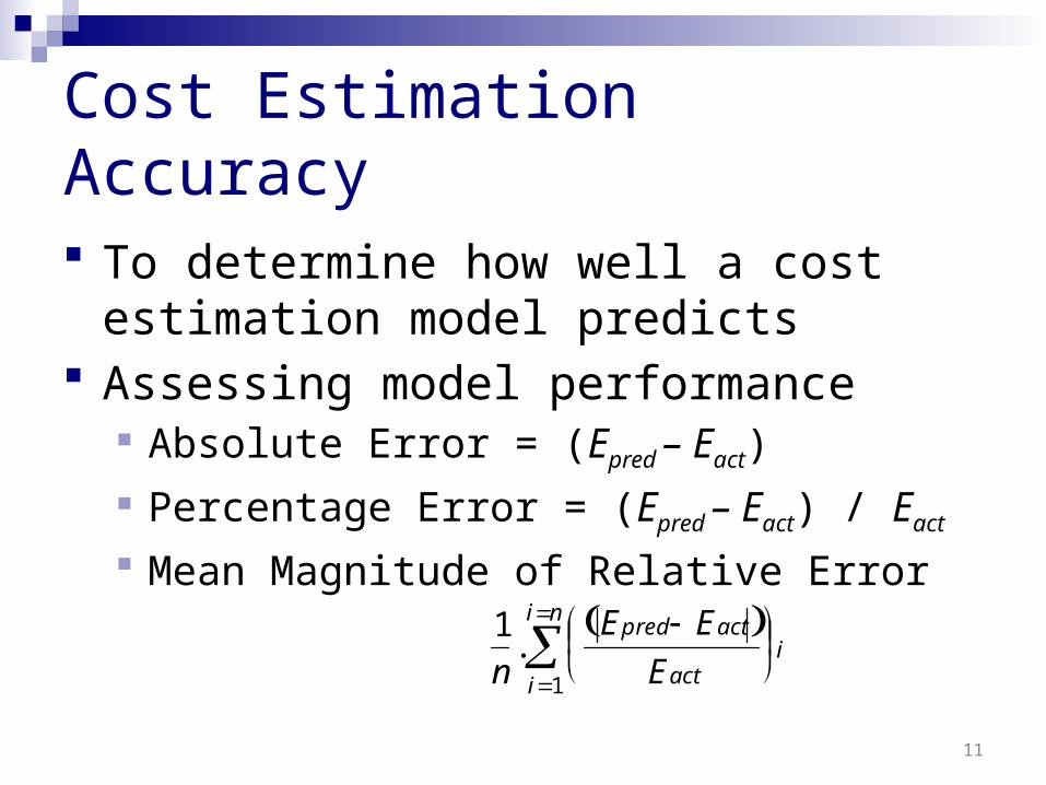
Cost Estimation Accuracy

To determine how well a cost estimation model predicts

Assessing model performance Absolute Error = (Epred – Eact)

Percentage Error = (Epred – Eact) / Eact

Mean Magnitude of Relative Error

1n.

Epred Eact Eact

i1

in

i

12

Cost Estimation Methods

Algorithmic (Parametric) model Expert Judgment (Expertise Based) Top – Down Bottom – Up Estimation by Analogy Price to Win Estimation

13

Algorithmic (Parametric) Model

Use of mathematical equations to perform software estimation

Equations are based on theory or historical data Use input such as SLOC, number of functions to

perform and other cost drivers Accuracy of model can be improved by

calibrating the model to the specific environment

14

Algorithmic (Parametric) Model (Cont.) Examples:

COCOMO (COnstructive COst MOdel) Developed by Boehm in 1981 Became one of the most popular and most transparent cost

model Mathematical model based on the data from 63 historical

software project COCOMO II

Published in 1995 To address issue on non-sequential and rapid development

process models, reengineering, reuse driven approaches, object oriented approach etc

Has three submodels – application composition, early design and post-architecture

15

Algorithmic (Parametric) Model (Cont.)

Putnam’s software life-cycle model (SLIM) Developed in the late 1970s Based on the Putnam’s analysis of the life-cycle in

terms of a so-called Rayleigh distribution of project personnel level versus time.

Quantitative software management developed three tools : SLIM-Estimate, SLIM-Control and SLIM-Metrics.

16

Algorithmic (Parametric) Model (Cont.) Advantages

Generate repeatable estimations Easy to modify input data Easy to refine and customize formulas Objectively calibrated to experience

Disadvantages Unable to deal with exceptional conditions Some experience and factors can not be quantified Sometimes algorithms may be proprietary

17

Expert Judgment

Capture the knowledge and experience of the practitioners and providing estimates based upon all the projects to which the expert participated.

Examples Delphi

Developed by Rand Corporation in 1940 where participants are involved in two assessment rounds.

Work Breakdown Structure (WBS) A way of organizing project element into a hierarchy that

simplifies the task of budget estimation and control

18

Expert Judgment (Cont.)

Advantages Useful in the absence of quantified, empirical data. Can factor in differences between past project

experiences and requirements of the proposed project Can factor in impacts caused by new technologies,

applications and languages. Disadvantages

Estimate is only as good expert’s opinion Hard to document the factors used by the experts

19

Top - Down

Also called Macro Model Derived from the global properties of the

product and then partitioned into various low level components

Example – Putnam model

20

Top – Down (Cont.)

Advantages Requires minimal project detail Usually faster and easier to implement Focus on system level activities

Disadvantages Tend to overlook low level components No detailed basis

21

Bottom - Up

Cost of each software components is estimated and then combine the results to arrive the total cost for the project

The goal is to construct the estimate of the system from the knowledge accumulated about the small software components and their interactions

An example – COCOMO’s detailed model

22

Bottom – Up (Cont.)

Advantages More stable More detailed Allow each software group to hand an

estimate Disadvantages

May overlook system level costs More time consuming

23

Estimation by Analogy

Comparing the proposed project to previously completed similar project in the same application domain

Actual data from the completed projects are extrapolated

Can be used either at system or component level

24

Estimation by Analogy (Cont.)

Advantages Based on actual project data

Disadvantages Impossible if no comparable project had been

tackled in the past. How well does the previous project represent

this one

25

Price to Win Estimation

Price believed necessary to win the contract

Advantages Often rewarded with the contract

Disadvantages Time and money run out before the job is

done

26

COCOMO 81 COCOMO stands for COnstructive

COst MOdel It is an open system First published by

Dr Barry Bohem in 1981 Worked quite well for projects in the

80’s and early 90’s Could estimate results within ~20% of

the actual values 68% of the time

27

COCOMO 81 COCOMO has three different models (each one

increasing with detail and accuracy): Basic, applied early in a project Intermediate, applied after requirements are specified. Advanced, applied after design is complete

COCOMO has three different modes: Organic – “relatively small software teams develop

software in a highly familiar, in-house environment” [Bohem]

Embedded – operate within tight constraints, product is strongly tied to “complex of hardware, software, regulations, and operational procedures” [Bohem]

Semi-detached – intermediate stage somewhere between organic and embedded. Usually up to 300 KDSI

28

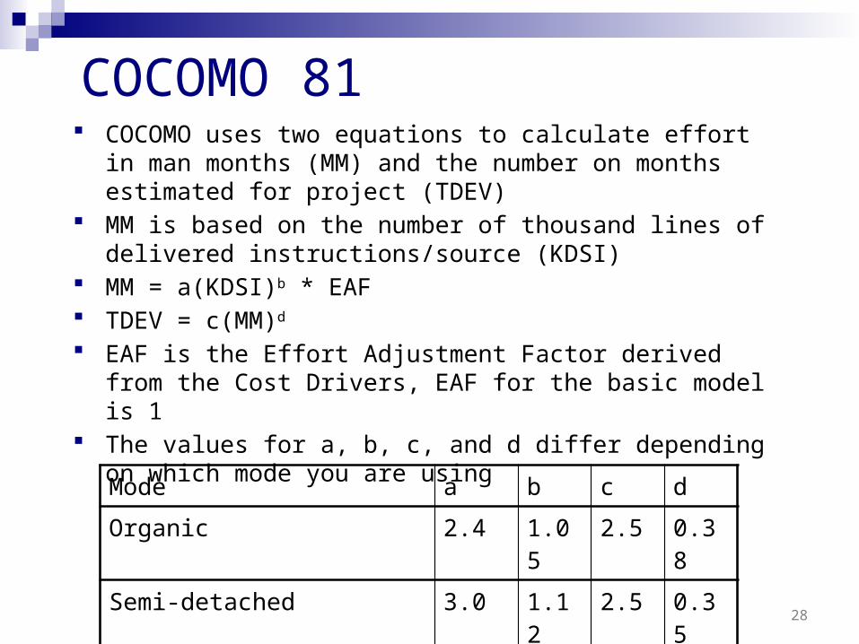
COCOMO 81 COCOMO uses two equations to calculate effort in man months

(MM) and the number on months estimated for project (TDEV) MM is based on the number of thousand lines of delivered

instructions/source (KDSI) MM = a(KDSI)b * EAF TDEV = c(MM)d

EAF is the Effort Adjustment Factor derived from the Cost Drivers, EAF for the basic model is 1

The values for a, b, c, and d differ depending on which mode you are using

Mode a b c d

Organic 2.4 1.05 2.5 0.38

Semi-detached 3.0 1.12 2.5 0.35

Embedded 3.6 1.20 2.5 0.32

29

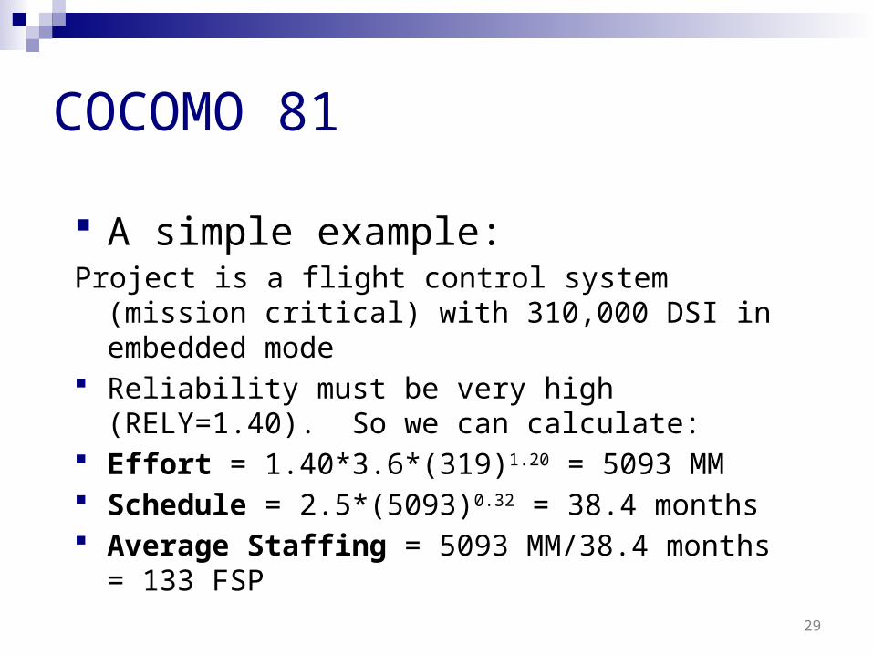
COCOMO 81

A simple example:Project is a flight control system (mission critical) with

310,000 DSI in embedded mode Reliability must be very high (RELY=1.40).  So we

can calculate: Effort = 1.40*3.6*(319)1.20 = 5093 MM Schedule = 2.5*(5093)0.32 = 38.4 months Average Staffing = 5093 MM/38.4 months = 133

FSP

30

COCOMO Conclusions

COCOMO is the most popular software cost estimation method

Easy to do, small estimates can be done by hand

USC has a free graphical version available for download

Many different commercial version based on COCOMO – they supply support and more data, but at a price

31

Conclusions

Project costs are being poorly estimated The accuracy of cost estimation has to be

improved Data collection Use of tools

Use several methods of estimation