Embed Size (px)
Citation preview
1
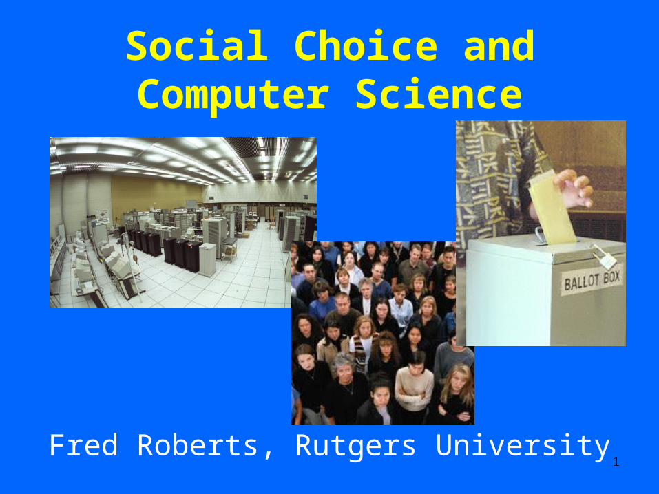
Social Choice and Computer Science
Fred Roberts, Rutgers University

2
Thank you to our hosts!
3
I’m sorry if you’d rather be watching futbol.
4
I’m sorry if you’d rather be watching futbol.
5
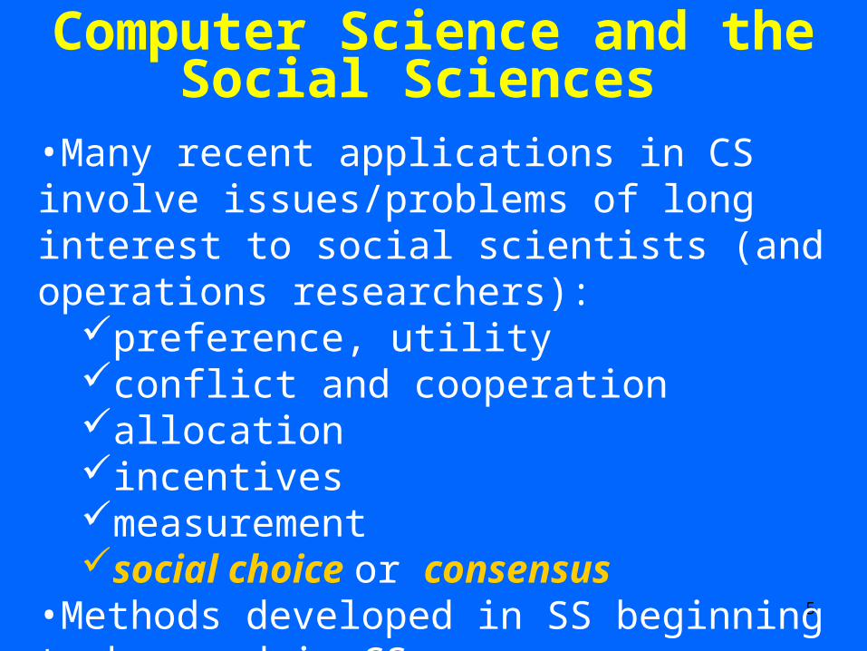
Computer Science and the Social Sciences
•Many recent applications in CS involve issues/problems of long interest to social scientists (and operations researchers):
preference, utilityconflict and cooperationallocationincentivesmeasurementsocial choice or consensus
•Methods developed in SS beginning to be used in CS
6
CS and SS •CS applications place great strain on SS methods
Sheer size of problems addressedComputational power of agents an issueLimitations on information possessed by playersSequential nature of repeated applications
•Thus: Need for new generation of SS methods
•Also: These new methods will provide powerful tools to social scientists
7
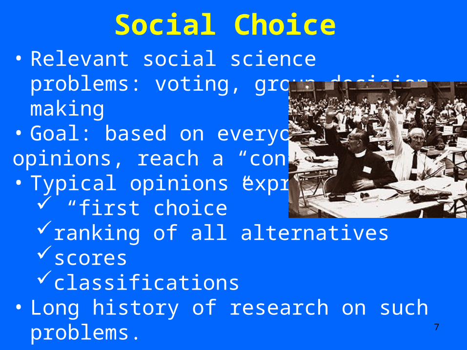
Social Choice • Relevant social science problems: voting, group
decision making• Goal: based on everyone’s opinions, reach a “consensus” • Typical opinions expressed as:
“first choice”ranking of all alternativesscores classifications
• Long history of research on such problems.

8
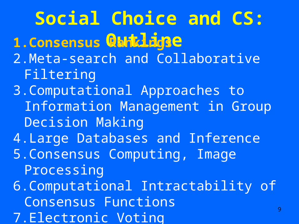
Social Choice and CS: Outline 1.Consensus Rankings2.Meta-search and Collaborative Filtering3.Computational Approaches to Information
Management in Group Decision Making4.Large Databases and Inference5.Consensus Computing, Image Processing6.Computational Intractability of Consensus
Functions7.Electronic Voting8.Software and Hardware Measurement9.Power of a Voter
9
Social Choice and CS: Outline 1.Consensus Rankings2.Meta-search and Collaborative Filtering3.Computational Approaches to Information
Management in Group Decision Making4.Large Databases and Inference5.Consensus Computing, Image Processing6.Computational Intractability of Consensus
Functions7.Electronic Voting8.Software and Hardware Measurement9.Power of a Voter
10
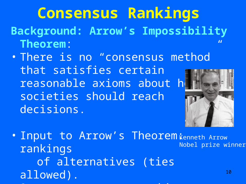
Consensus Rankings Background: Arrow’s Impossibility Theorem: • There is no “consensus method” that satisfies
certain reasonable axioms about how societies should reach decisions.
• Input to Arrow’s Theorem: rankings of alternatives (ties allowed).• Output: consensus ranking.
Kenneth ArrowNobel prize winner
11
Consensus Rankings
• There are widely studied and widely used consensus methods (that violate one or
more of Arrow’s conditions).
• One well-known consensus method: “Kemeny-Snell medians”: Given set of rankings, find ranking minimizing sum of distances to other rankings.
• Kemeny-Snell medians are having surprising new applications in CS.
John Kemeny,pioneer in time sharingin CS
12
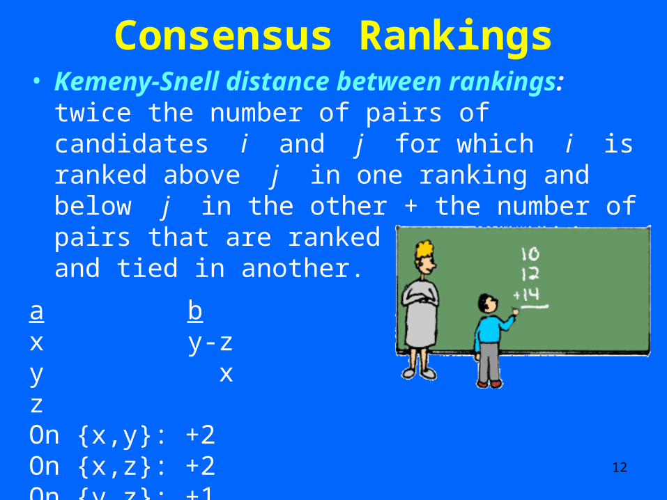
Consensus Rankings• Kemeny-Snell distance between rankings: twice the
number of pairs of candidates i and j for which i is ranked above j in one ranking and below j in the other + the number of pairs that are ranked in one ranking and tied in another.
a bx y-zy xzOn {x,y}: +2On {x,z}: +2On {y,z}: +1d(a,b) = 5.
13
Consensus Rankings
• Kemeny-Snell median: Given rankings a1, a2, …, ap, find a ranking x so that
d(a1,x) + d(a2,x) + … + d(ap,x) is minimized.
• x can be a ranking other than a1, a2, …, ap.
• Sometimes just called Kemeny median.
14
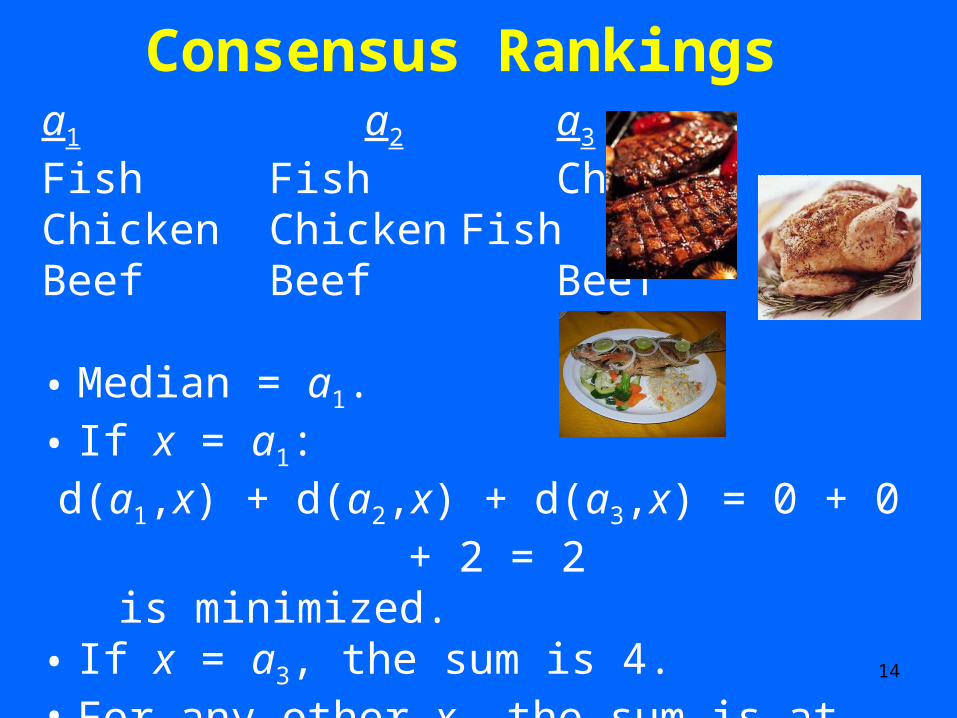
Consensus Rankings a1 a2 a3
Fish Fish ChickenChicken Chicken FishBeef Beef Beef
• Median = a1.
• If x = a1:d(a1,x) + d(a2,x) + d(a3,x) = 0 + 0 + 2 = 2
is minimized.• If x = a3, the sum is 4.• For any other x, the sum is at least 1 + 1 + 1 = 3.
15
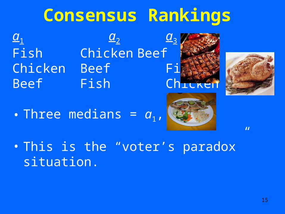
Consensus Rankings a1 a2 a3
Fish Chicken BeefChicken Beef FishBeef Fish Chicken
• Three medians = a1, a2, a3.
• This is the “voter’s paradox” situation.
16
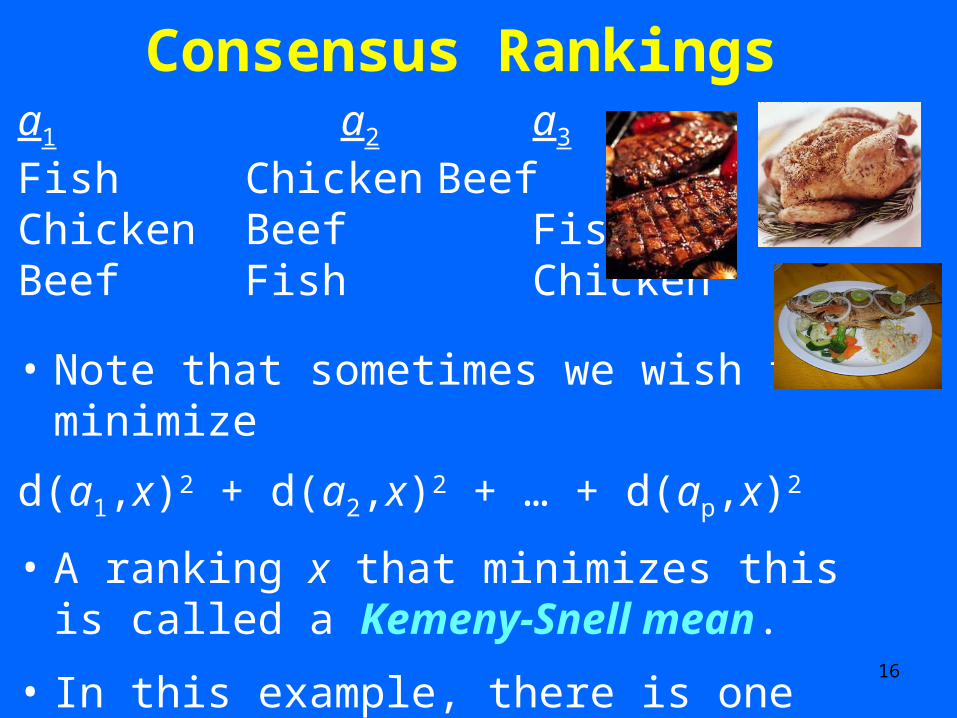
Consensus Rankings a1 a2 a3
Fish Chicken BeefChicken Beef FishBeef Fish Chicken
• Note that sometimes we wish to minimize
d(a1,x)2 + d(a2,x)2 + … + d(ap,x)2
• A ranking x that minimizes this is called a Kemeny-Snell mean.
• In this example, there is one mean: the ranking declaring all three alternatives tied.
17
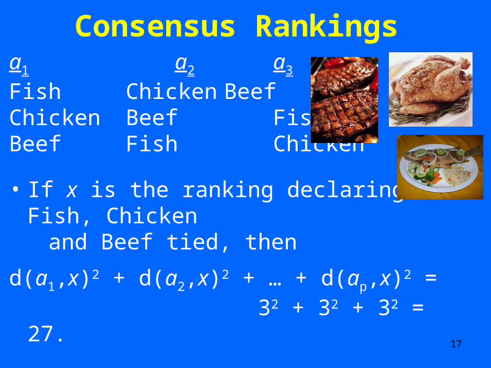
Consensus Rankings a1 a2 a3
Fish Chicken BeefChicken Beef FishBeef Fish Chicken
• If x is the ranking declaring Fish, Chicken and Beef tied, then
d(a1,x)2 + d(a2,x)2 + … + d(ap,x)2 = 32 + 32 + 32 = 27.
• Not hard to show this is minimum.
18
Consensus Rankings
Theorem (Bartholdi, Tovey, and Trick, 1989; Wakabayashi, 1986): Computing the Kemeny median of a set of rankings is an NP-complete problem.
19
Consensus Rankings
Okay, so what does this have to do with practical computer science questions?
20
Consensus Rankings
I mean really practical computer science questions.
21
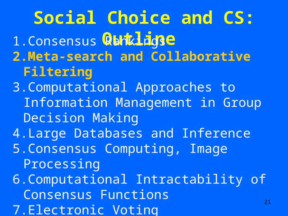
Social Choice and CS: Outline 1.Consensus Rankings2.Meta-search and Collaborative Filtering3.Computational Approaches to Information
Management in Group Decision Making4.Large Databases and Inference5.Consensus Computing, Image Processing6.Computational Intractability of Consensus
Functions7.Electronic Voting8.Software and Hardware Measurement9.Power of a Voter
22
Meta-search and Collaborative Filtering Meta-search
• A consensus problem• Combine page rankings from several search
engines• Dwork, Kumar, Naor, Sivakumar (2000):
Kemeny-Snell medians good in spam resistance in meta-search (spam by a page if it causes meta-search to rank it too highly)
• Approximation methods make this computationally tractable
23
Meta-search and Collaborative Filtering
Collaborative Filtering
• Recommending books or movies• Combine book or movie ratings• Produce ordered list of books or movies to
recommend• Freund, Iyer, Schapire, Singer (2003):
“Boosting” algorithm for combining rankings.• Related topic: Recommender Systems
24
Meta-search and Collaborative Filtering
A major difference from SS applications:
• In SS applications, number of voters is large, number of candidates is small.
• In CS applications, number of voters (search engines) is small, number of candidates (pages) is large.
• This makes for major new complications and research challenges.
25
Social Choice and CS: Outline 1.Consensus Rankings2.Meta-search and Collaborative Filtering3.Computational Approaches to Information
Management in Group Decision Making4.Large Databases and Inference5.Consensus Computing, Image Processing6.Computational Intractability of Consensus
Functions7.Electronic Voting8.Software and Hardware Measurement9.Power of a Voter
26
Computational Approaches to Information Management in Group Decision Making
Representation and Elicitation
• Successful group decision making (social choice) requires efficient elicitation of information and efficient representation of the information elicited.
• Old problems in the social sciences.• Computational aspects becoming a focal point
because of need to deal with massive and complex information.
27
Computational Approaches to Information Management in Group Decision Making
Representation and Elicitation
• Example I: Social scientists study preferences: “I prefer beef to fish”
• Extracting and representing preferences is key in group decision making applications.
28
Computational Approaches to Information Management in Group Decision Making
Representation and Elicitation
• “Brute force” approach: For every pair of alternatives, ask which is preferred to the other.
• Often computationally infeasible.
29
Computational Approaches to Information Management in Group Decision Making
Representation and Elicitation
• In many applications (e.g., collaborative filtering), important to elicit preferences automatically.
• CP-nets introduced as tool to represent preferences succinctly and provide ways to make inferences about preferences (Boutilier, Brafman, Doomshlak, Hoos, Poole 2004).
30
Computational Approaches to Information Management in Group Decision Making
Representation and Elicitation
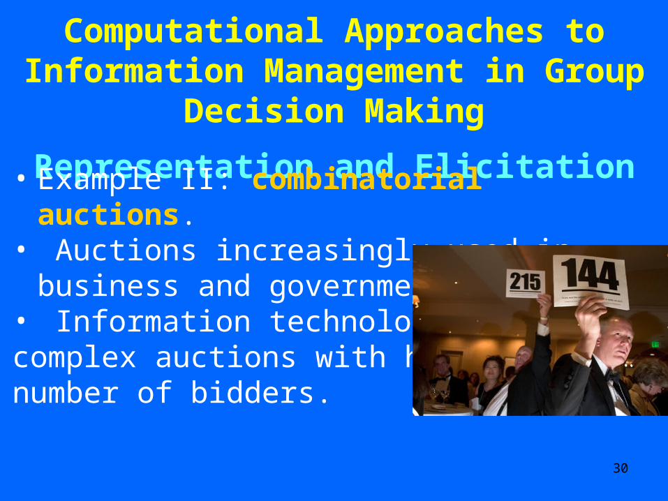
• Example II: combinatorial auctions.• Auctions increasingly used in business and
government.• Information technology allows complex auctions with huge number of bidders.
31
Computational Approaches to Information Management in Group Decision Making
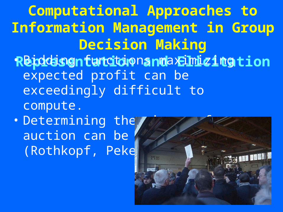
Representation and Elicitation• Bidding functions maximizing expected profit
can be exceedingly difficult to compute.• Determining the winner of an auction can be
extremely hard. (Rothkopf, Pekec, Harstad 1998)
32
Computational Approaches to Information Management in Group Decision Making
Representation and Elicitation
Combinatorial Auctions
• Multiple goods auctioned off.• Submit bids for combinations of goods.• This leads to NP-complete allocation problems.• Might not even be able to feasibly express all
possible preferences for all subsets of goods.• Rothkopf, Pekec, Harstad (1998): determining
winner is computationally tractable for many economically interesting kinds of combinations.

33
Computational Approaches to Information Management in Group Decision Making
Representation and Elicitation
Combinatorial Auctions
• Decision maker needs to elicit preferences from all agents for all plausible combinations of items in the auction.
• Similar problem arises in optimal bundling of goods and services.
• Elicitation requires exponentially many queries in general.
34
Computational Approaches to Information Management in Group Decision Making
Representation and Elicitation• Challenge: Recognize situations in which
efficient elicitation and representation is possible.
• One result: Fishburn, Pekec, Reeds (2002)• Even more complicated: When objects in
auction have complex structure. • Problem arises in:
Legal reasoning, sequential decision making, automatic decision devices, collaborative filtering.
35
Social Choice and CS: Outline 1.Consensus Rankings2.Meta-search and Collaborative Filtering3.Computational Approaches to Information
Management in Group Decision Making4.Large Databases and Inference5.Consensus Computing, Image Processing6.Computational Intractability of Consensus
Functions7.Electronic Voting8.Software and Hardware Measurement9.Power of a Voter

36
Large Databases and Inference • Real data often in form of sequences• Here, concentrate on bioinformatics• GenBank has over 7 million sequences
comprising 8.6 billion bases. • The search for similarity or patterns has
extended from pairs of sequences to finding patterns that appear in common in a large number of sequences or throughout the database: “consensus sequences”.
• Emerging field of “Bioconsensus”: applies SS consensus methods to biological databases.
37
Large Databases and Inference
Why look for such patterns?
Similarities between sequences or parts of sequences lead to the discovery of shared phenomena.
For example, it was discovered that the sequence for platelet derived factor, which causes growth in the body, is 87% identical to the sequence for v-sis, a cancer-causing gene. This led to the discovery that v-sis works by stimulating growth.
38
Large Databases and Inference Example
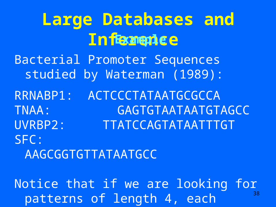
Bacterial Promoter Sequences studied by Waterman (1989):
RRNABP1: ACTCCCTATAATGCGCCATNAA: GAGTGTAATAATGTAGCCUVRBP2: TTATCCAGTATAATTTGTSFC: AAGCGGTGTTATAATGCC
Notice that if we are looking for patterns of length 4, each sequence has the pattern TAAT.
39
Large Databases and Inference Example
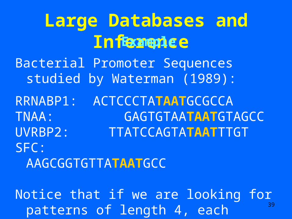
Bacterial Promoter Sequences studied by Waterman (1989):
RRNABP1: ACTCCCTATAATGCGCCATNAA: GAGTGTAATAATGTAGCCUVRBP2: TTATCCAGTATAATTTGTSFC: AAGCGGTGTTATAATGCC
Notice that if we are looking for patterns of length 4, each sequence has the pattern TAAT.
40
Large Databases and Inference Example
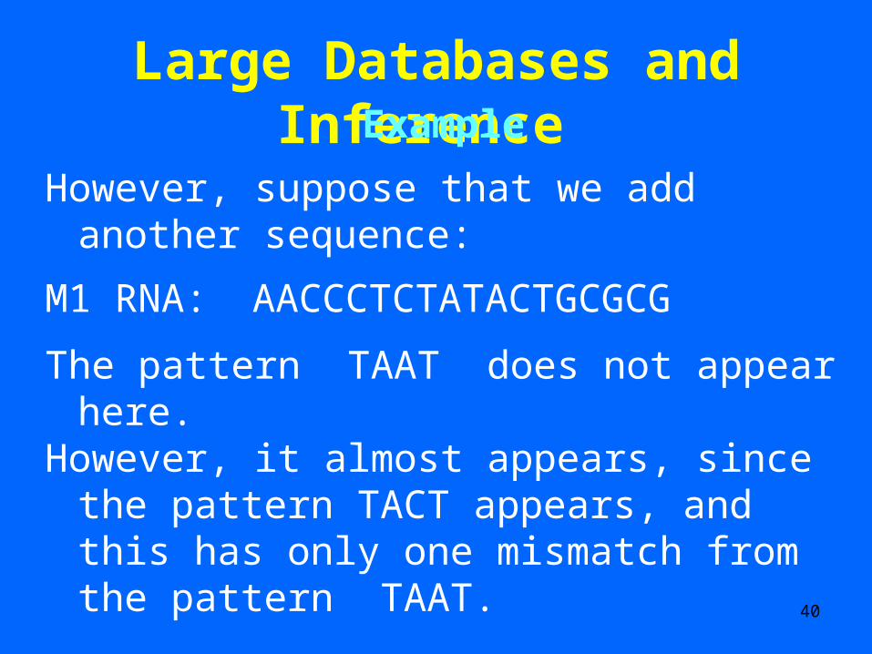
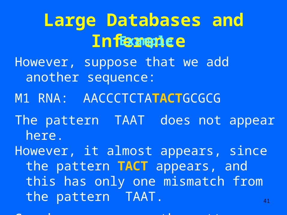
However, suppose that we add another sequence:
M1 RNA: AACCCTCTATACTGCGCG
The pattern TAAT does not appear here.However, it almost appears, since the pattern
TACT appears, and this has only one mismatch from the pattern TAAT.
41
Large Databases and Inference Example
However, suppose that we add another sequence:
M1 RNA: AACCCTCTATACTGCGCG
The pattern TAAT does not appear here.However, it almost appears, since the pattern
TACT appears, and this has only one mismatch from the pattern TAAT.
So, in some sense, the pattern TAAT is a good consensus pattern.
42
Large Databases and Inference Example
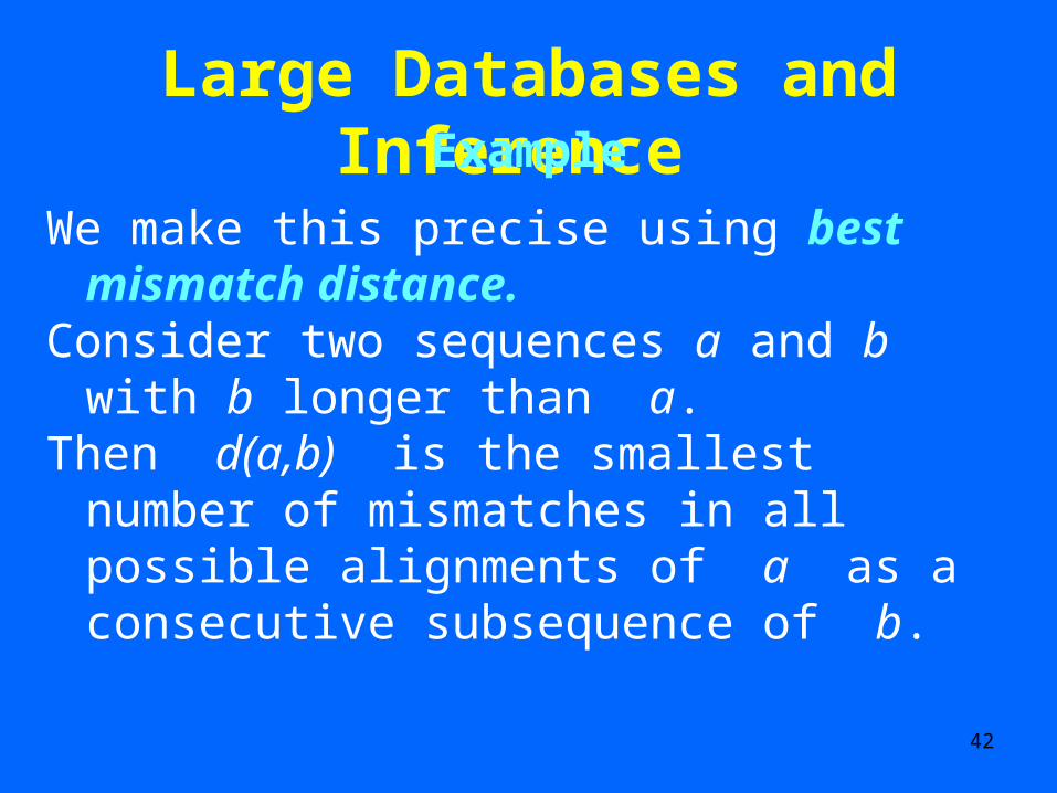
We make this precise using best mismatch distance.
Consider two sequences a and b with b longer than a.
Then d(a,b) is the smallest number of mismatches in all possible alignments of a as a consecutive subsequence of b.
43
Large Databases and Inference Example
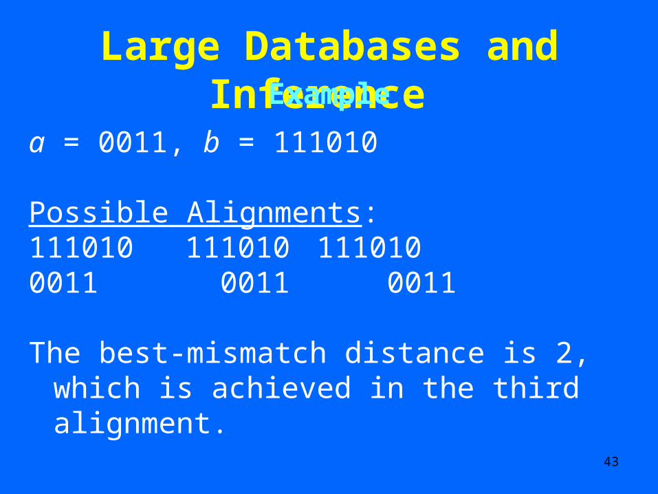
a = 0011, b = 111010
Possible Alignments:111010111010 1110100011 0011 0011
The best-mismatch distance is 2, which is achieved in the third alignment.
44
Large Databases and Inference Smith-Waterman
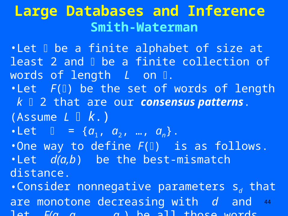
•Let be a finite alphabet of size at least 2 and be a finite collection of words of length L on . •Let F() be the set of words of length k 2 that are our consensus patterns. (Assume L k.)•Let = {a1, a2, …, an}. •One way to define F() is as follows. •Let d(a,b) be the best-mismatch distance. •Consider nonnegative parameters sd that are monotone decreasing with d and let F(a1,a2, …, an) be all those words w of length k that maximize
S(w) = isd(w,ai)
45
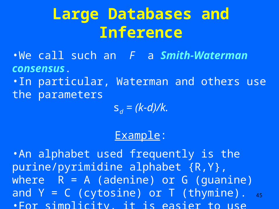
Large Databases and Inference•We call such an F a Smith-Waterman consensus.•In particular, Waterman and others use the parameters
sd = (k-d)/k.
Example:
•An alphabet used frequently is the purine/pyrimidine alphabet {R,Y}, where R = A (adenine) or G (guanine) and Y = C (cytosine) or T (thymine). •For simplicity, it is easier to use the digits 0,1 rather than the letters R,Y.
•Thus, let = {0,1}, let k = 2. Then the possible pattern words are 00, 01, 10, 11.
46
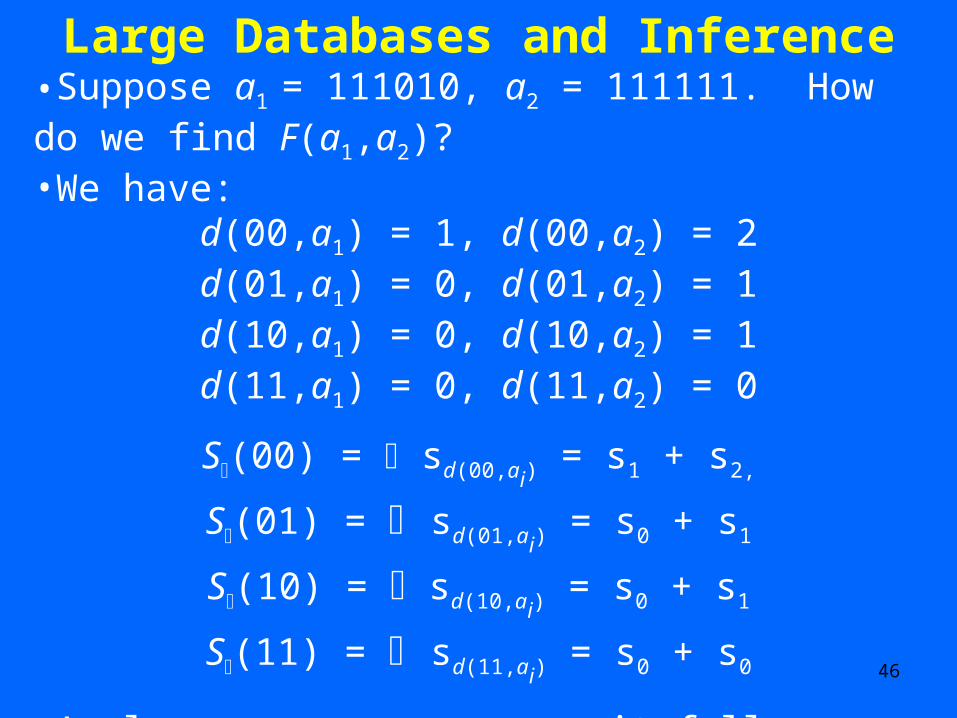
Large Databases and Inference•Suppose a1 = 111010, a2 = 111111. How do we find F(a1,a2)?•We have:
d(00,a1) = 1, d(00,a2) = 2d(01,a1) = 0, d(01,a2) = 1d(10,a1) = 0, d(10,a2) = 1d(11,a1) = 0, d(11,a2) = 0
S(00) = sd(00,ai) = s1 + s2,
S(01) = sd(01,ai) = s0 + s1
S(10) = sd(10,ai) = s0 + s1
S(11) = sd(11,ai) = s0 + s0
•As long as s0 > s1 > s2, it follows that 11 is the consensus pattern, according to Smith-Waterman’s consensus.
47
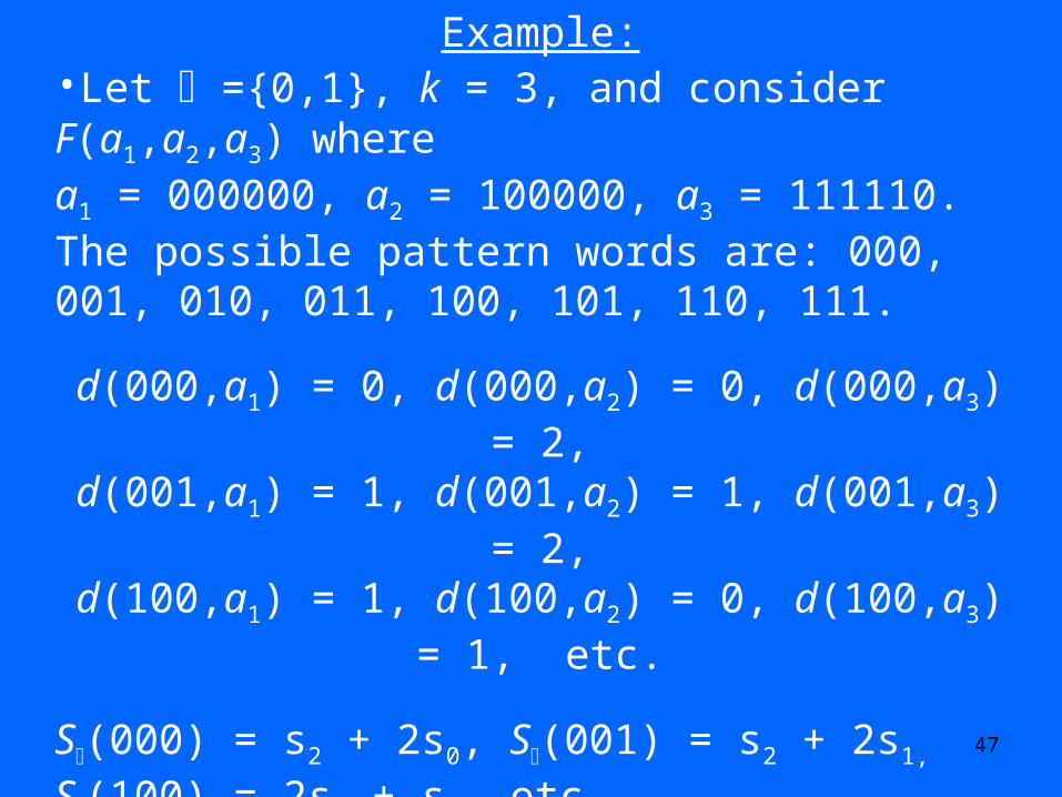
Example:•Let ={0,1}, k = 3, and consider F(a1,a2,a3) where a1 = 000000, a2 = 100000, a3 = 111110. The possible pattern words are: 000, 001, 010, 011, 100, 101, 110, 111.
d(000,a1) = 0, d(000,a2) = 0, d(000,a3) = 2,d(001,a1) = 1, d(001,a2) = 1, d(001,a3) = 2,
d(100,a1) = 1, d(100,a2) = 0, d(100,a3) = 1, etc.
S(000) = s2 + 2s0, S(001) = s2 + 2s1, S(100) = 2s1 + s0, etc.
•Now, s0 > s1 > s2 implies that S(000) > S(001). •Similarly, one shows that the score is maximized by S(000) or S(100). • Monotonicity doesn’t say which of these is highest.
48
Large Databases and Inference
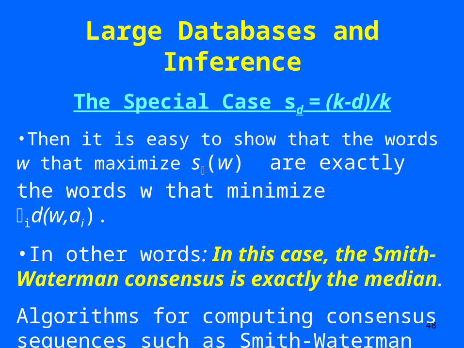
The Special Case sd = (k-d)/k
•Then it is easy to show that the words w that maximize s(w) are exactly the words w that minimize
id(w,ai).
•In other words: In this case, the Smith-Waterman consensus is exactly the median.
Algorithms for computing consensus sequences such as Smith-Waterman are important in modern molecular biology.
49
Large Databases and Inference Other Topics in “Bioconsensus”
• Alternative phylogenies (evolutionary trees) are produced using different methods and we need to choose a consensus tree.
• Alternative taxonomies (classifications) are produced using different models and we need to choose a consensus taxonomy.
• Alternative molecular sequences are produced using different criteria or different algorithms and we need to choose a consensus sequence.
• Alternative sequence alignments are produced and we need to choose a consensus alignment.
50
Large Databases and Inference
Other Topics in “Bioconsensus”
• Several recent books on bioconsensus.• Day and McMorris [2003]• Janowitz, et al. [2003]
• Bibliography compiled by Bill Day: In molecular biology alone, hundreds of papers using consensus methods in biology.
• Large database problems in CS are being approached using methods of “bioconsensus” having their origin in the social sciences.
51
Social Choice and CS: Outline 1.Consensus Rankings2.Meta-search and Collaborative Filtering3.Computational Approaches to Information
Management in Group Decision Making4.Large Databases and Inference5.Consensus Computing, Image Processing6.Computational Intractability of Consensus
Functions7.Electronic Voting8.Software and Hardware Measurement9.Power of a Voter
52
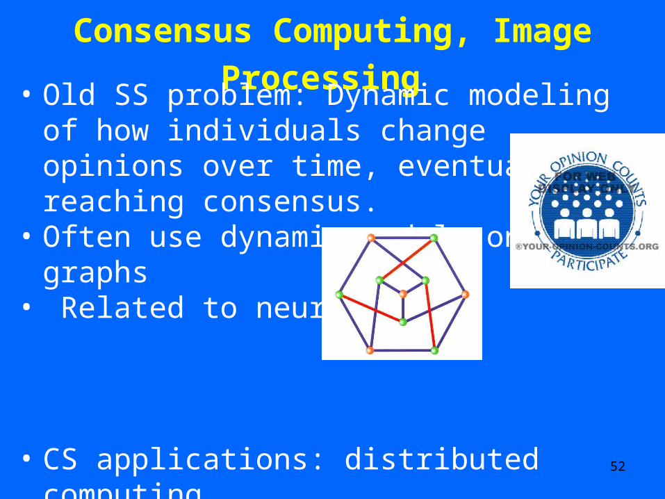
Consensus Computing, Image Processing • Old SS problem: Dynamic modeling of how
individuals change opinions over time, eventually reaching consensus.
• Often use dynamic models on graphs• Related to neural nets.
• CS applications: distributed computing.• Values of processors in a network are updated
until all have same value.
53
Consensus Computing, Image Processing • CS application: Noise removal in digital images• Does a pixel level represent noise?• Compare neighboring pixels.• If values beyond threshold, replace pixel value
with mean or median of values of neighbors.• Related application in distributed computing.• Values of faulty processors are replaced by those
of neighboring non-faulty ones.• Berman and Garay (1993) use “parliamentary
procedure” called cloture
54
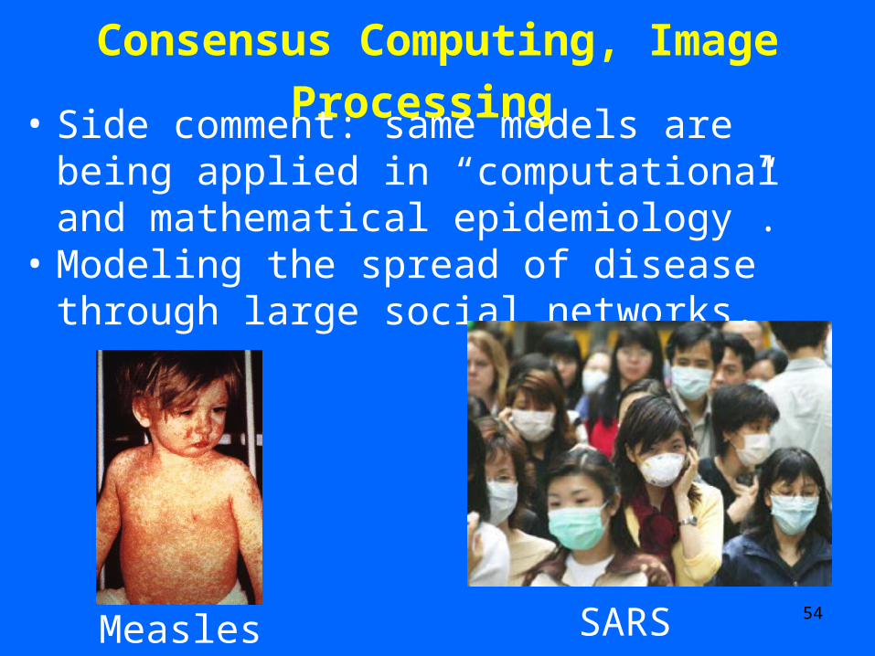
Consensus Computing, Image Processing • Side comment: same models are being applied in
“computational and mathematical epidemiology”.
• Modeling the spread of disease through large social networks.
SARSMeasles
55
Social Choice and CS: Outline 1.Consensus Rankings2.Meta-search and Collaborative Filtering3.Computational Approaches to Information
Management in Group Decision Making4.Large Databases and Inference5.Consensus Computing, Image Processing6.Computational Intractability of Consensus
Functions7.Electronic Voting8.Software and Hardware Measurement9.Power of a Voter
56
Computational Intractability of Consensus Functions
• How hard is it to compute the winner of an election?
• We know counting votes can be difficult and time consuming. • However:
• Bartholdi, Tovey and Trick (1989): There are voting schemes where it can be computationally intractable to determine who won an election.
57
Computational Intractability of Consensus Functions
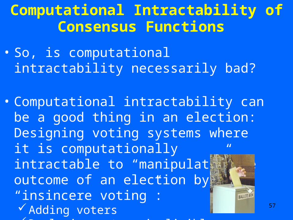
• So, is computational intractability necessarily bad?
• Computational intractability can be a good thing in an election: Designing voting systems where it is computationally intractable to “manipulate” the outcome of an election by “insincere voting”:Adding votersDeclaring voters ineligibleAdding candidatesDeclaring candidates ineligible
58
Computational Intractability of Consensus Functions
• Given a set A of all possible candidates and a set I of all possible voters.
• Suppose we know voter i’s ranking of all candidates in A, for every voter i.
• Given a subset of I of eligible voters, a particular candidate a in A, and a number k, is there a set of at most k ineligible voters who can be declared eligible so that candidate a is the winner?
• Bartholdi, Tovey, Trick (1989): For some consensus functions (voting rules), this is an NP-complete problem.
59
Computational Intractability of Consensus Functions
• Given a set A of all possible candidates and a set I of all possible voters.
• Suppose we know voter i’s ranking of all candidates in A, for every voter i.
• Given a subset of I of eligible voters, a particular candidate a in A, and a number k, is there a set of at most k eligible voters who can be declared ineligible so that candidate a is the winner?
• Bartholdi, Tovey, Trick (1989): For some consensus functions (voting rules), this is an NP-complete problem.
60
Computational Intractability of Consensus Functions
• Software agents may be more likely to manipulate than individuals (Conitzer and Sandholm 2002):Humans don’t think about manipulatingComputation can be tedious.Software agents are good at running
algorithmsSoftware agents only need to have code for
manipulation written once.All the more reason to develop
computational barriers to manipulation.
61
Computational Intractability of Consensus Functions
• Stopping those software agents:
62
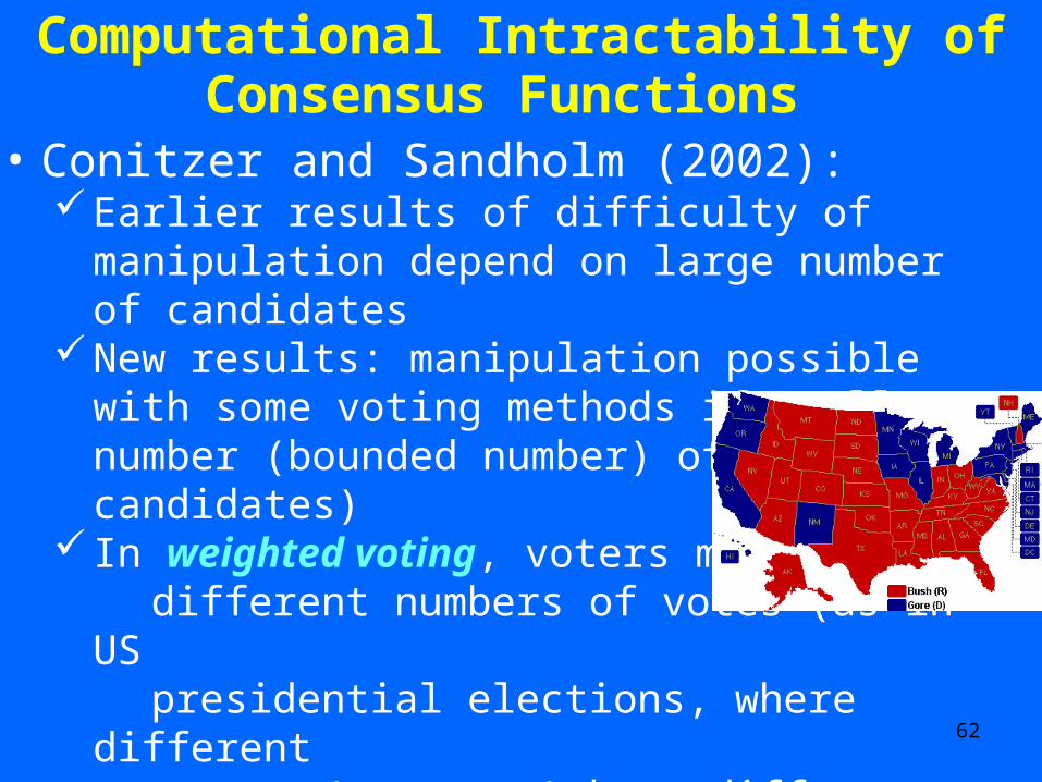
Computational Intractability of Consensus Functions
• Conitzer and Sandholm (2002):Earlier results of difficulty of manipulation depend
on large number of candidatesNew results: manipulation possible with some
voting methods if smaller number (bounded number) of candidates)
In weighted voting, voters may have different numbers of votes (as in US presidential elections, where different states (= voters) have different numbers of votes). Here, manipulation is harder.Manipulation difficult when uncertainty about
others’ votes.
63
Computational Intractability of Consensus Functions
• Conitzer and Sandholm (2006):Try to find voting rules for which
manipulation is usually hard.Why is this difficult to do?One explanation: under one reasonable
assumption, it is impossible to find such rules.
64
Social Choice and CS: Outline 1.Consensus Rankings2.Meta-search and Collaborative Filtering3.Computational Approaches to Information
Management in Group Decision Making4.Large Databases and Inference5.Consensus Computing, Image Processing6.Computational Intractability of Consensus
Functions7.Electronic Voting8.Software and Hardware Measurement9.Power of a Voter
65
Aside: Electronic Voting
• Issues:CorrectnessAnonymityAvailabilitySecurityPrivacy
66
Electronic VotingSecurity Risks in Electronic Voting
• Threat of “denial of service attacks”• Threat of penetration attacks involving a
delivery mechanism to transport a malicious payload to target host (thru Trojan horse or remote control program)
• Private and correct counting of votes• Cryptographic challenges to keep votes private• Relevance of work on secure multiparty
computation
67
Electronic Voting
Other CS Challenges:
• Resistance to “vote buying”• Development of user-friendly interfaces• Vulnerabilities of communication path between
the voting client (where you vote) and the server (where votes are counted)
• Reliability issues: random hardware and software failures

68
Social Choice and CS: Outline 1.Consensus Rankings2.Meta-search and Collaborative Filtering3.Computational Approaches to Information
Management in Group Decision Making4.Large Databases and Inference5.Consensus Computing, Image Processing6.Computational Intractability of Consensus
Functions7.Electronic Voting8.Software and Hardware Measurement9.Power of a Voter
69
Software & Hardware Measurement • Theory of measurement developed by
mathematical social scientists• Measurement theory studies ways to combine
scores obtained on different criteria.• A statement involving scales of measurement is considered meaningful if its
truth or falsity is unchanged under acceptable transformations of all scales involved.
• Example: It is meaningful to say that I weigh more than my daughter.
• That is because if it is true in kilograms, then it is also true in pounds, in grams, etc.
70
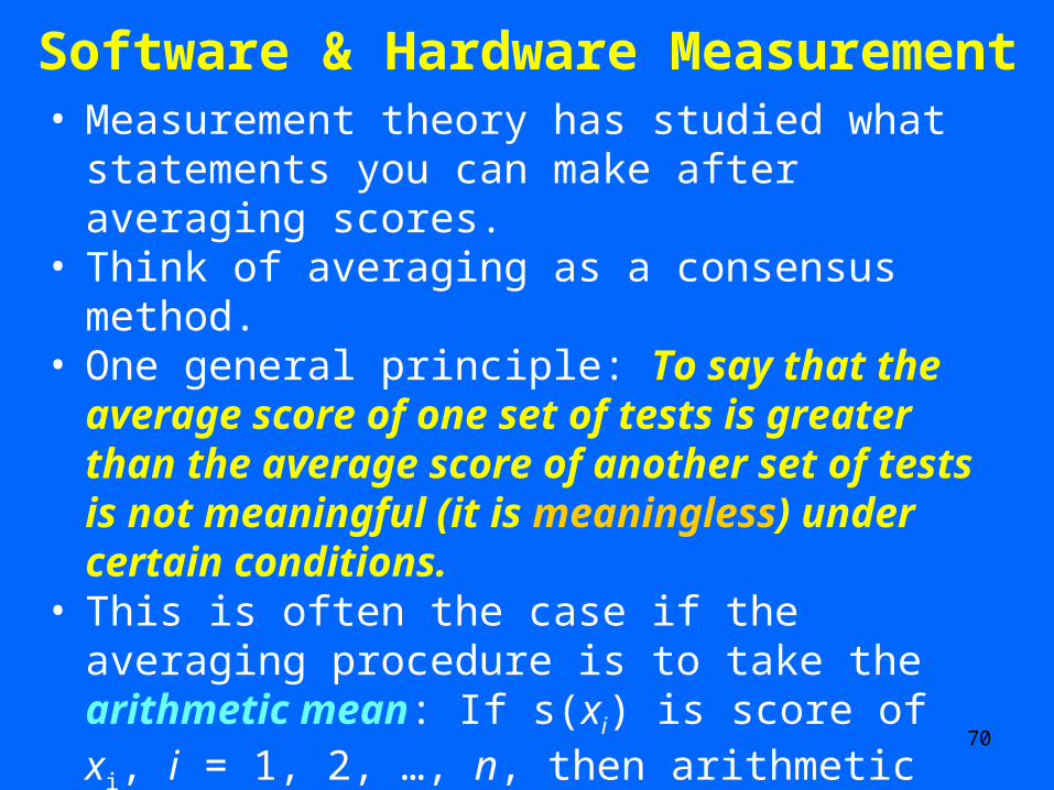
Software & Hardware Measurement • Measurement theory has studied what statements you
can make after averaging scores.• Think of averaging as a consensus method.• One general principle: To say that the average score of
one set of tests is greater than the average score of another set of tests is not meaningful (it is meaningless) under certain conditions.
• This is often the case if the averaging procedure is to take the arithmetic mean: If s(xi) is score of xi, i = 1, 2, …, n, then arithmetic mean is
is(xi)/n.• Long literature on what averaging methods lead to
meaningful conclusions.
71
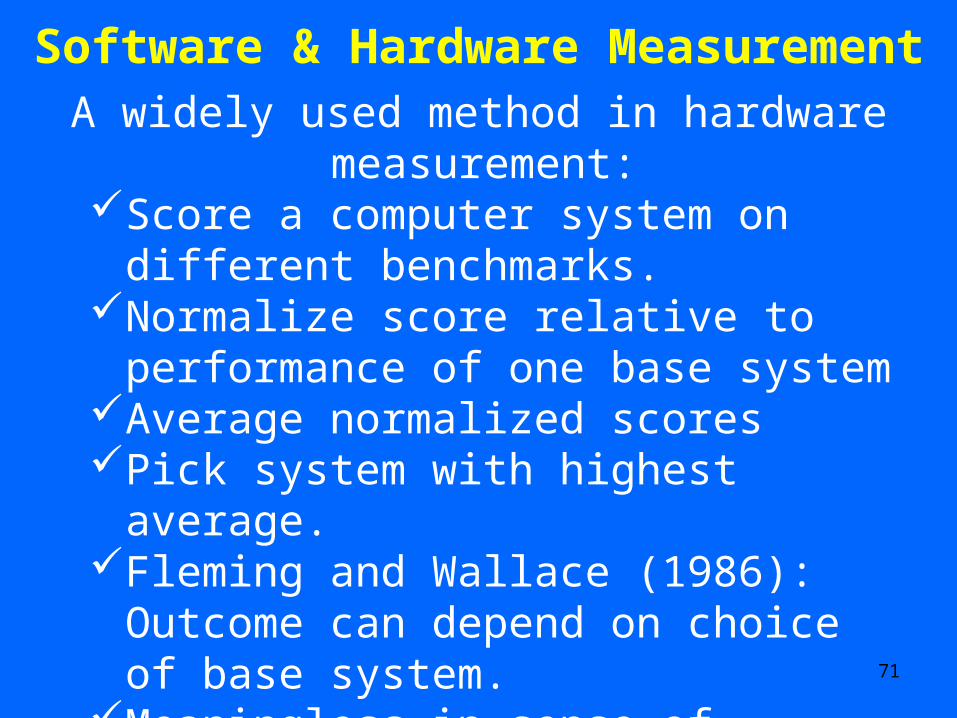
Software & Hardware Measurement A widely used method in hardware measurement:
Score a computer system on different benchmarks.
Normalize score relative to performance of one base system
Average normalized scoresPick system with highest average.Fleming and Wallace (1986): Outcome can
depend on choice of base system. Meaningless in sense of measurement theoryLeads to theory of merging normalized scores

72
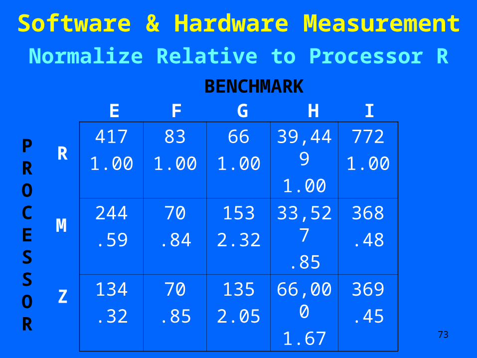
Software & Hardware Measurement Hardware Measurement
417 83 66 39,449 772
244 70 153 33,527 368
134 70 135 66,000 369
BENCHMARK
R
M
Z
PROCESSOR
E F G H I
Data from Heath, Comput. Archit. News (1984)
73
Software & Hardware Measurement Normalize Relative to Processor R
417
1.00
83
1.00
66
1.00
39,449
1.00
772
1.00
244
.59
70
.84
153
2.32
33,527
.85
368
.48
134
.32
70
.85
135
2.05
66,000
1.67
369
.45
BENCHMARK
R
M
Z
PROCESSOR
E F G H I
74
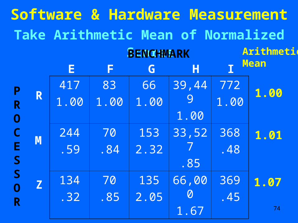
Software & Hardware Measurement Take Arithmetic Mean of Normalized Scores
417
1.00
83
1.00
66
1.00
39,449
1.00
772
1.00
244
.59
70
.84
153
2.32
33,527
.85
368
.48
134
.32
70
.85
135
2.05
66,000
1.67
369
.45
BENCHMARK
R
M
Z
PROCESSOR
E F G H I
ArithmeticMean
1.00
1.01
1.07
75
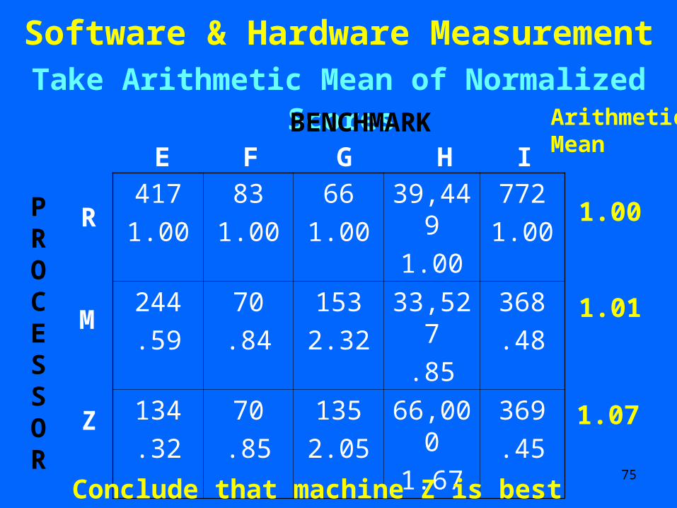
Software & Hardware Measurement Take Arithmetic Mean of Normalized Scores
417
1.00
83
1.00
66
1.00
39,449
1.00
772
1.00
244
.59
70
.84
153
2.32
33,527
.85
368
.48
134
.32
70
.85
135
2.05
66,000
1.67
369
.45
BENCHMARK
R
M
Z
PROCESSOR
E F G H I
ArithmeticMean
1.00
1.01
1.07
Conclude that machine Z is best
76
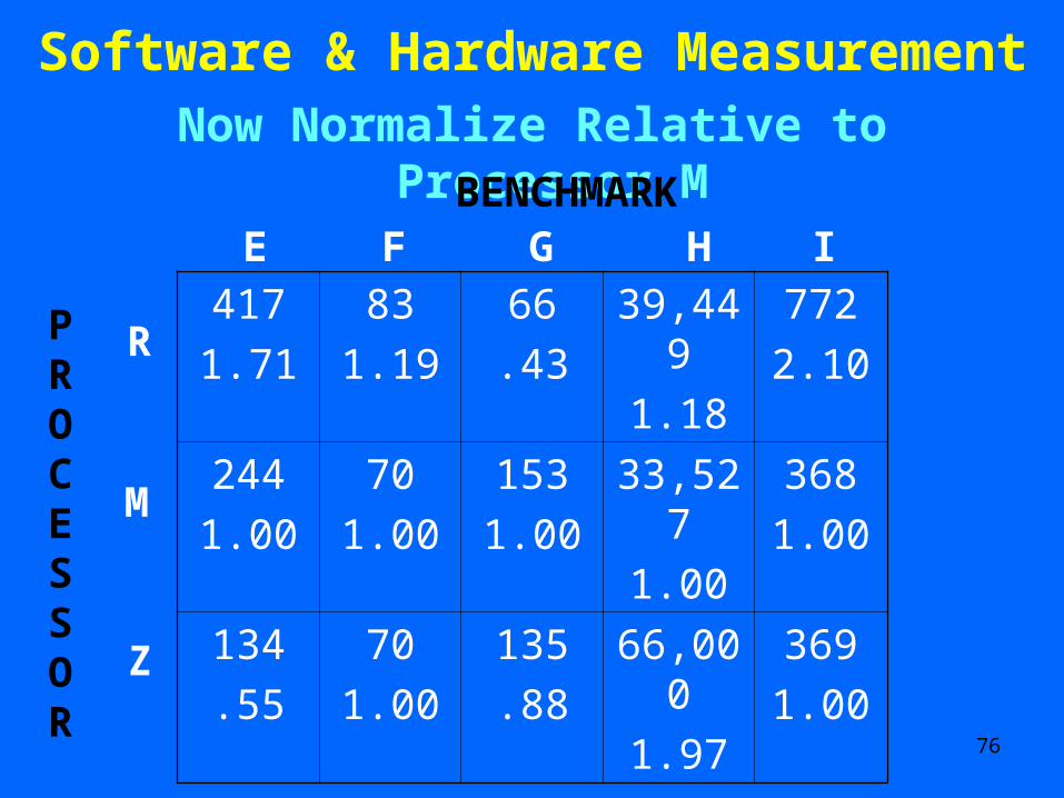
Software & Hardware Measurement Now Normalize Relative to Processor M
417
1.71
83
1.19
66
.43
39,449
1.18
772
2.10
244
1.00
70
1.00
153
1.00
33,527
1.00
368
1.00
134
.55
70
1.00
135
.88
66,000
1.97
369
1.00
BENCHMARK
R
M
Z
PROCESSOR
E F G H I
77
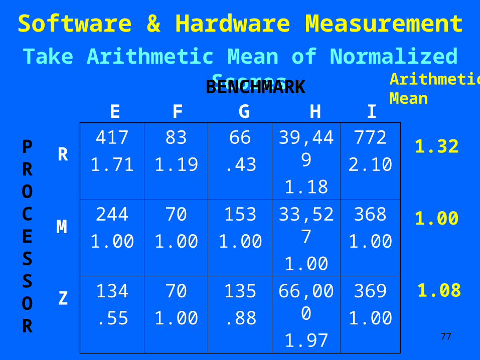
Software & Hardware Measurement Take Arithmetic Mean of Normalized Scores
417
1.71
83
1.19
66
.43
39,449
1.18
772
2.10
244
1.00
70
1.00
153
1.00
33,527
1.00
368
1.00
134
.55
70
1.00
135
.88
66,000
1.97
369
1.00
BENCHMARK
R
M
Z
PROCESSOR
E F G H I
ArithmeticMean
1.32
1.00
1.08
78
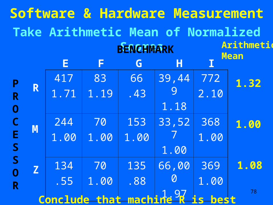
Software & Hardware Measurement Take Arithmetic Mean of Normalized Scores
417
1.71
83
1.19
66
.43
39,449
1.18
772
2.10
244
1.00
70
1.00
153
1.00
33,527
1.00
368
1.00
134
.55
70
1.00
135
.88
66,000
1.97
369
1.00
BENCHMARK
R
M
Z
PROCESSOR
E F G H I
ArithmeticMean
1.32
1.00
1.08
Conclude that machine R is best
79
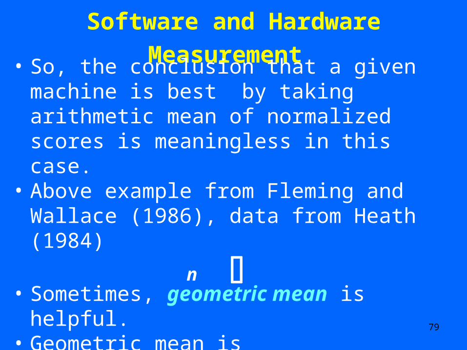
Software and Hardware Measurement • So, the conclusion that a given machine is best
by taking arithmetic mean of normalized scores is meaningless in this case.
• Above example from Fleming and Wallace (1986), data from Heath (1984)
• Sometimes, geometric mean is helpful.• Geometric mean is
is(xi)n
80
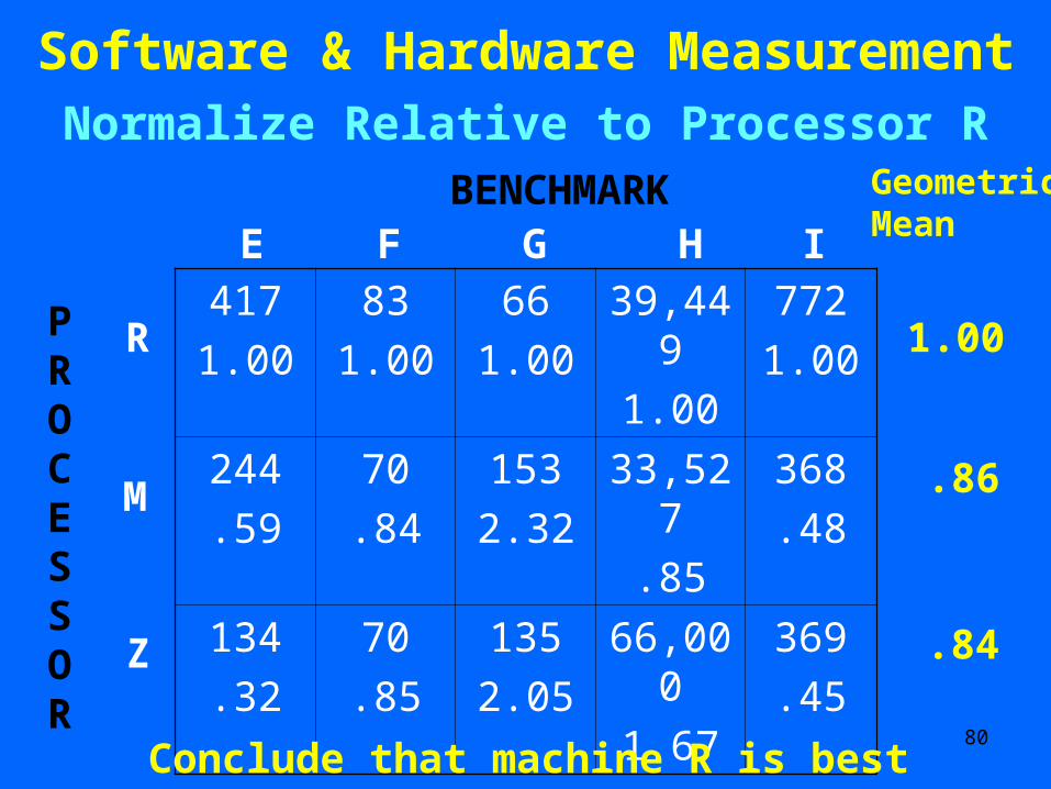
Software & Hardware Measurement Normalize Relative to Processor R
417
1.00
83
1.00
66
1.00
39,449
1.00
772
1.00
244
.59
70
.84
153
2.32
33,527
.85
368
.48
134
.32
70
.85
135
2.05
66,000
1.67
369
.45
BENCHMARK
R
M
Z
PROCESSOR
E F G H I
GeometricMean
1.00
.86
.84
Conclude that machine R is best
81
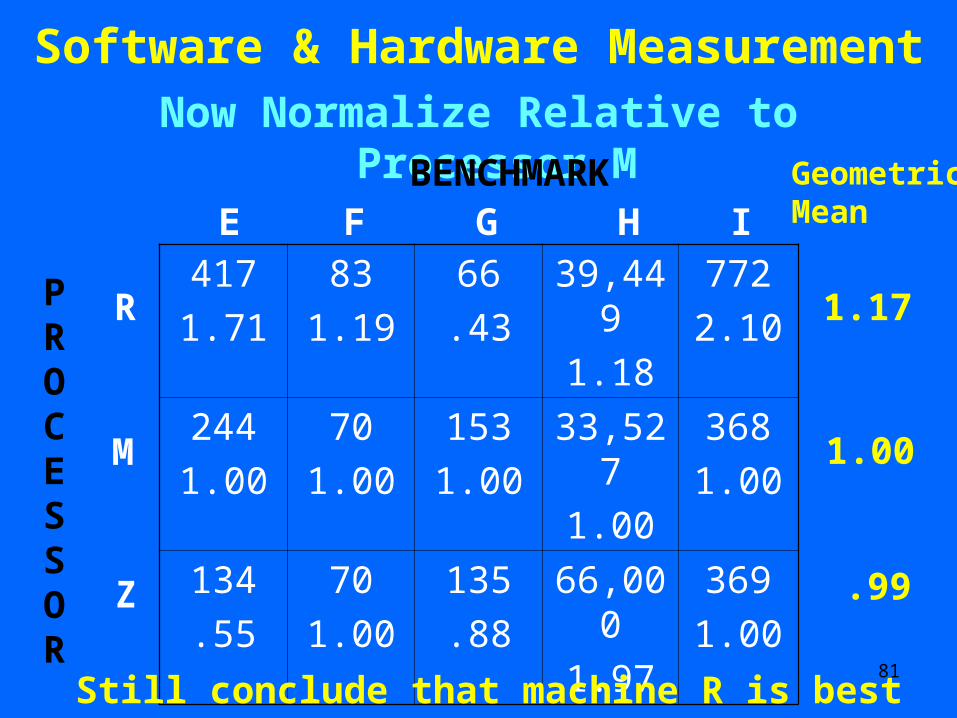
Software & Hardware Measurement Now Normalize Relative to Processor M
417
1.71
83
1.19
66
.43
39,449
1.18
772
2.10
244
1.00
70
1.00
153
1.00
33,527
1.00
368
1.00
134
.55
70
1.00
135
.88
66,000
1.97
369
1.00
BENCHMARK
R
M
Z
PROCESSOR
E F G H IGeometricMean
1.17
1.00
.99
Still conclude that machine R is best
82
Software and Hardware Measurement• In this situation, it is easy to show that the conclusion
that a given machine has highest geometric mean normalized score is a meaningful conclusion.
• Even meaningful: A given machine has geometric mean normalized score 20% higher than another machine.
• Fleming and Wallace give general conditions under which comparing geometric means of normalized scores is meaningful.
• Research area: what averaging procedures make sense in what situations? Large literature.
• Note: There are situations where comparing arithmetic means is meaningful but comparing geometric means is not.
83
Software and Hardware Measurement
• Message from measurement theory to computer science (and O.R.):
Do not perform arithmetic operations on data without paying attention to whether the conclusions you get are meaningful.
84
Social Choice and CS: Outline 1.Consensus Rankings2.Meta-search and Collaborative Filtering3.Computational Approaches to Information
Management in Group Decision Making4.Large Databases and Inference5.Consensus Computing, Image Processing6.Computational Intractability of Consensus
Functions7.Electronic Voting8.Software and Hardware Measurement9.Power of a Voter
85
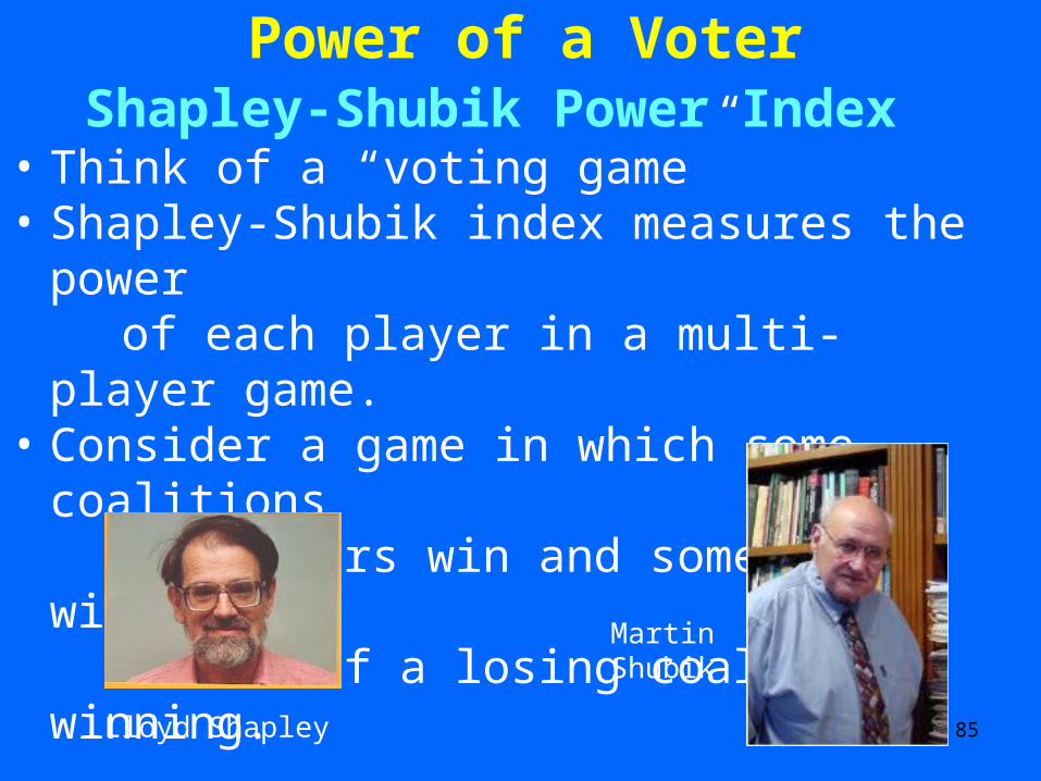
Power of a VoterShapley-Shubik Power Index
• Think of a “voting game”• Shapley-Shubik index measures the power of each player in a multi-player game.• Consider a game in which some coalitions of players win and some lose, with no subset of a losing coalition winning.
Lloyd Shapley
MartinShubik
86
Power of a Voter
Shapley-Shubik Power Index• Consider a coalition forming at random, one
player at a time.• A player i is pivotal if addition of i throws
coalition from losing to winning. • Shapley-Shubik index of i = probability i is
pivotal if an order of players is chosen at random.
• Power measure applying to more general games than voting games is called Shapley Value.
87
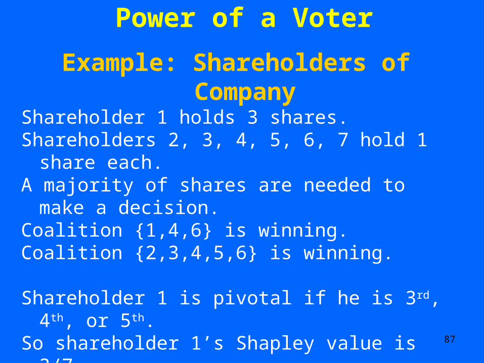
Power of a Voter
Example: Shareholders of CompanyShareholder 1 holds 3 shares.Shareholders 2, 3, 4, 5, 6, 7 hold 1 share each.A majority of shares are needed to make a decision.Coalition {1,4,6} is winning.Coalition {2,3,4,5,6} is winning.
Shareholder 1 is pivotal if he is 3rd, 4th, or 5th.So shareholder 1’s Shapley value is 3/7.Sum of Shapley values is 1 (since they are probabilities)Thus, each other shareholder has Shapley value
(4/7)/6 = 2/21
88
Power of a Voter
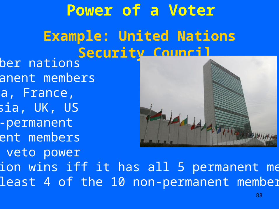
Example: United Nations Security Council
•15 member nations•5 permanent members
China, France, Russia, UK, US
•10 non-permanent•Permanent members have veto power•Coalition wins iff it has all 5 permanent membersand at least 4 of the 10 non-permanent members.

89
Power of a Voter
Example: United Nations Security Council
•What is the power of eachMember of the SecurityCouncil? •Fix non-permanent member i.•i is pivotal in permutations in which all permanent members precede i and exactly 3 non- permanent members do.•How many such permutations are there?
90
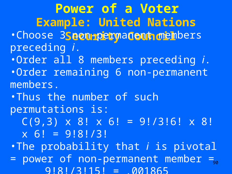
Power of a VoterExample: United Nations Security Council•Choose 3 non-permanent members preceding i. •Order all 8 members preceding i.•Order remaining 6 non-permanent members.•Thus the number of such permutations is:
C(9,3) x 8! x 6! = 9!/3!6! x 8! x 6! = 9!8!/3!•The probability that i is pivotal = power of non-permanent member =
9!8!/3!15! = .001865•The power of a permanent member =
[1 – 10 x .001865]/5 = .1963.•Permanent members have 100 times power of non-permanent members.
91
Power of a Voter
•There are a variety of other power indices used in game theory and political science (Banzhaf index, Coleman index, …)
•Need calculate them for huge games•Mostly computationally intractable
92
Power of a Voter: Allocation/Sharing Costs and Revenues
• Shapley-Shubik power index and more general Shapley value have been used to allocate costs to different users in shared projects.Allocating runway fees in airportsAllocating highway fees to trucks of
different sizesUniversities sharing library facilitiesFair allocation of telephone calling
charges among users sharing complex phone systems (Cornell’s experiment)

93
Power of a Voter: Allocating/Sharing Costs and Revenues
Allocating Runway Fees at Airports• Some planes require longer runways.
Charge them more for landings. How much more?
• Divide runways into meter-long segments.
• Each month, we know how many landings a plane has made.
• Given a runway of length y meters, consider a game in which the players are landings and a coalition “wins” if the runway is not long enough for planes in the coalition.

94
Power of a Voter: Allocating/Sharing Costs and Revenues
Allocating Runway Fees at Airports• A landing is pivotal if it is the first
landing added that makes a coalition require a longer runway.
• The Shapley value gives the cost of the yth meter of runway allocated to a given landing.
• We then add up these costs over all runway lengths a plane requires and all landings it makes.
95
Power of a Voter: Allocating/Sharing Costs and Revenues
Multicasting
• Applications in multicasting.• Unicast routing: Each packet sent from a
source is delivered to a single receiver.• Sending it to multiple sites: Send multiple
copies and waste bandwidth.• In multicast routing: Use a directed tree connecting source to all receivers.• At branch points, a packet is duplicated as necessary.
96
Multicasting
97
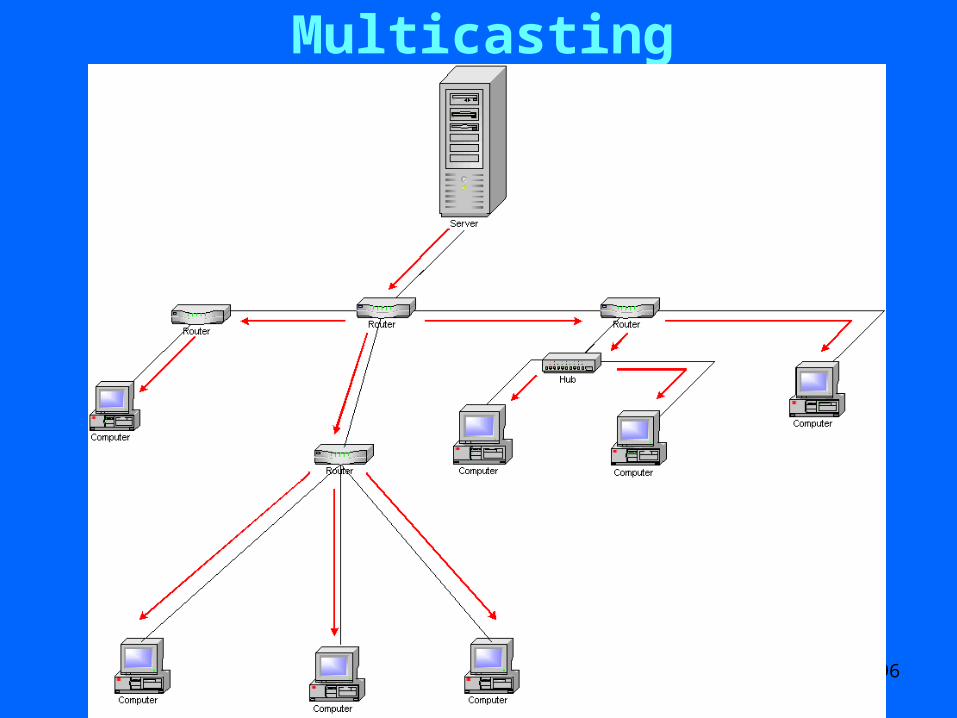
Power of a Voter: Allocating/Sharing Costs and Revenues
Multicasting
• Multicast routing: Use a directed tree connecting source to all receivers.
• At branch points, a packet is duplicated as necessary.
• Bandwidth is not directly attributable to a single receiver.
• How to distribute costs among receivers?• One idea: Use Shapley value.
98
Allocating/Sharing Costs and Revenues• Feigenbaum, Papadimitriou, Shenker (2001):
no feasible implementation for Shapley value in multicasting.
• Note: Shapley value is uniquely characterized by four simple axioms.
• Sometimes we state axioms as general principles we want a solution concept to have.
• Jain and Vazirani (1998): polynomial time computable cost-sharing algorithmSatisfying some important axiomsCalculating cost of optimum multicast tree within
factor of two of optimal.
99
Concluding Comment• In recent years, interplay between CS and biology has transformed major parts of Bio into an information science.• Led to major scientific breakthroughs in
biology such as sequencing of human genome.
• Led to significant new developments in CS, such as database search.
• The interplay between CS and SS not nearly as far along.
• Moreover: problems are spread over many disciplines.
100
Concluding Comment
• However, CS-SS interplay has already developed a unique momentum of its own.
• One can expect many more exciting outcomes as partnerships between computer scientists and social scientists expand and mature.

101