1

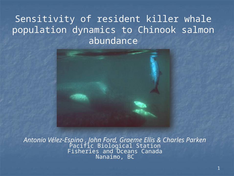
Sensitivity of resident killer whale population dynamics to Chinook salmon abundance

Antonio Vélez-Espino , John Ford, Graeme Ellis & Charles ParkenPacific Biological Station

Fisheries and Oceans CanadaNanaimo, BC

2

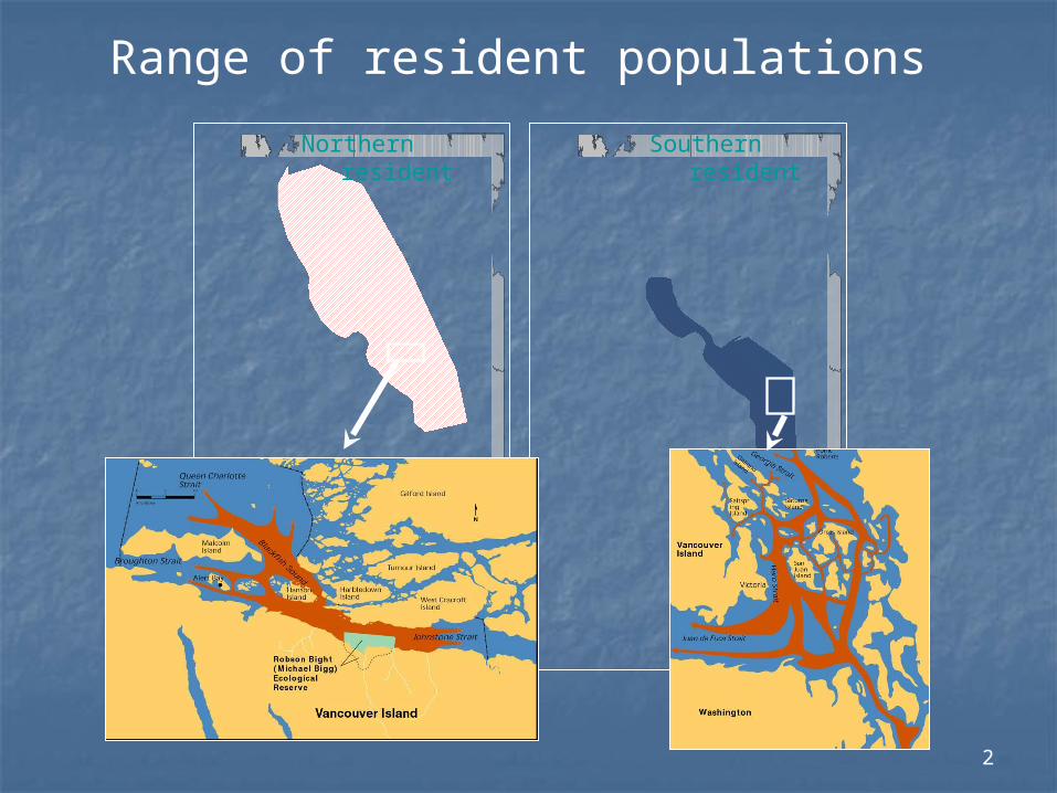
Northern resident Southern resident

Range of resident populations

3

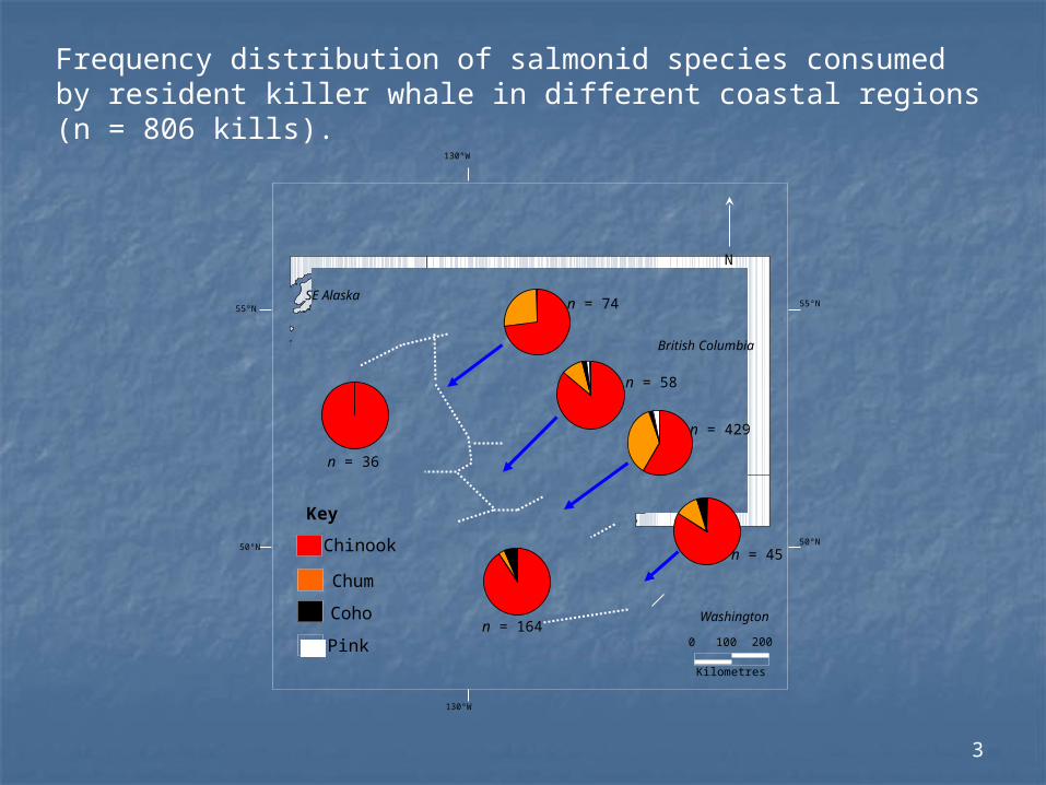
British Columbia

Washington

50°N 50°N

55°N 55°N

130°W

130°W

N

Kilometres

0 100 200

SE Alaska

Chinook

Chum

Coho

Pink

Key

n = 36

n = 74

n = 58

n = 429

n = 45

n = 164

Frequency distribution of salmonid species consumed by resident killer whale in different coastal regions (n = 806 kills).

4

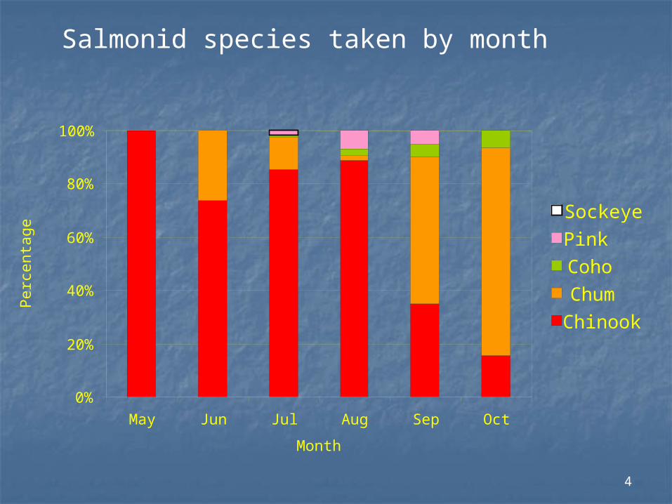
Salmonid species taken by month

0%

20%

40%

60%

80%

100%

May Jun Jul Aug Sep Oct

Month

Per

cent

age

Sockeye

Pink

Coho

Chum

Chinook

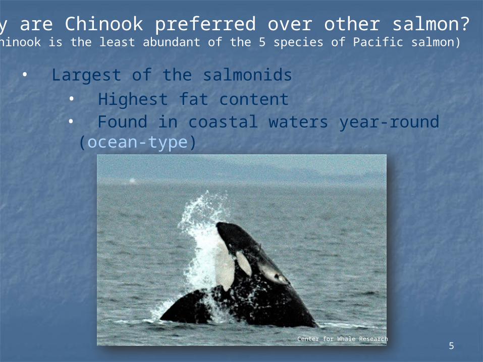
5

Why are Chinook preferred over other salmon?(Chinook is the least abundant of the 5 species of Pacific salmon)

Center for Whale Research

• Largest of the salmonids• Highest fat content• Found in coastal waters year-round (ocean-type)

6

Chinook GSI for SRKW

Hanson et al. (2010)

7

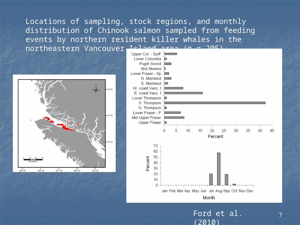
Locations of sampling, stock regions, and monthly distribution of Chinook salmon sampled from feeding events by northern resident killer whales in the northeastern Vancouver Island area (n = 205)

Ford et al. (2010)

8

Correlations between RKW vital rates & Chinook abundance detected by previous studies (Ford et al. 2010)

9

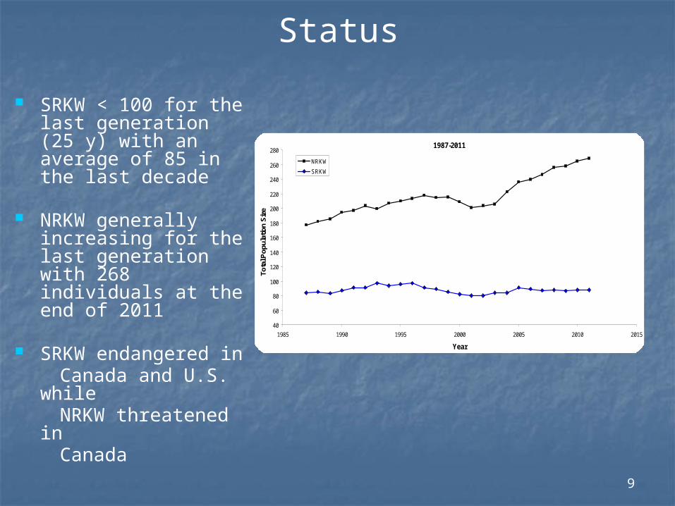
Status

SRKW < 100 for the last generation (25 y) with an average of 85 in the last decade

NRKW generally increasing for the last generation with 268 individuals at the end of 2011

SRKW endangered in Canada and U.S.

while NRKW threatened in Canada

1987-2011

40

60

80

100

120

140

160

180

200

220

240

260

280

1985 1990 1995 2000 2005 2010 2015

Year

Tota

l Pop

ulat

ion

Siz

e

NRKW

SRKW

10

THE QUESTIONS

• What are the demographic factors limiting population growth in SRKW and explaining the differences between both populations?

• What is the influence of Chinook salmon on the population dynamics of both SRKW and NRKW?

• How RKW populations are expected to respond to changes in Chinook fishing mortality?

M Malleson

11

Model Selection/Hypotheses

Life history dataGender-specific: age-at-maturity, maximum reproductive age,

maximum age

Stage-specific: survival, fecundity, growth

Vital rates (mean & variance)

Demographic projection matrices

SRKW and NRKW Chinook Salmon (Terminal Run, Ocean abundance)

Abundance datastock; stock aggregates

Relationships between Chinook abundance and vital rates

Perturbation analysis

Sensitivity of SRKW and NRKW population growth to

Chinook abundance

Retrospective(LTRE)

Prospective(i.e., elasticity)

Demographic factors responsible for observed

KW abundance variation

Relative importanceof stage-specific vital

rates for recoverypotential

12

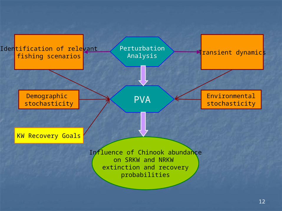
PerturbationAnalysis

Identification of relevantfishing scenarios

Transient dynamics

PVA Environmentalstochasticity

Demographic stochasticity

Influence of Chinook abundanceon SRKW and NRKW extinction and recovery

probabilities

KW Recovery Goals

13

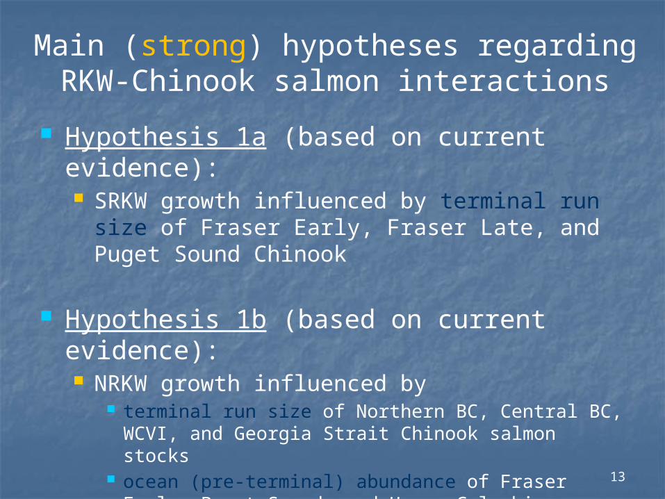
Main (strong) hypotheses regarding RKW-Chinook salmon interactions

Hypothesis 1a (based on current evidence): SRKW growth influenced by terminal run size of

Fraser Early, Fraser Late, and Puget Sound Chinook

Hypothesis 1b (based on current evidence): NRKW growth influenced by

terminal run size of Northern BC, Central BC, WCVI, and Georgia Strait Chinook salmon stocks

ocean (pre-terminal) abundance of Fraser Early, Puget Sound, and Upper Columbia Chinook stocks

14

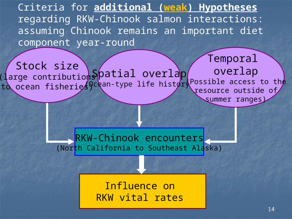
Criteria for additional (weak) Hypotheses regarding RKW-Chinook salmon interactions: assuming Chinook remains an important diet component year-round

RKW-Chinook encounters(North California to Southeast Alaska)

Influence on RKW vital rates

Stock size(large contributionsto ocean fisheries)

Spatial overlap(Ocean-type life history)

Temporal overlap

(Possible access to theresource outside of

summer ranges)

15

Killer Whale Demography

16

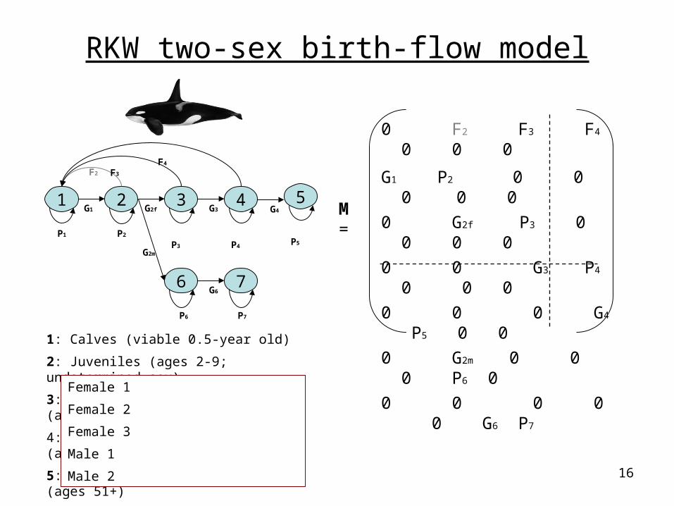
RKW two-sex birth-flow model

1: Calves (viable 0.5-year old)

2: Juveniles (ages 2-9; undetermined sex)

3: Young reproductive females (ages 10-30)

4: Old reproductive females (ages 31-50)

5: Post-reproductive females (ages 51+)

6: Young mature males (ages 10-21)

7: Old mature males (ages 22+)

1

6 7

2 43 G1 G2f G3

P2 P3 P4

F2

F3

G2m

G6

P6 P7

P1

0 F2 F3 F4 0 0 0

G1 P2 0 0 0 0 0

0 G2f P3 0 0 0 0

0 0 G3 P4 0 0 0

0 0 0 G4 P5 0 0

0 G2m 0 0 0 P6 0

0 0 0 0 0 G6 P7

M =5

P5

F4

G4

Female 1

Female 2

Female 3

Male 1

Male 2

17

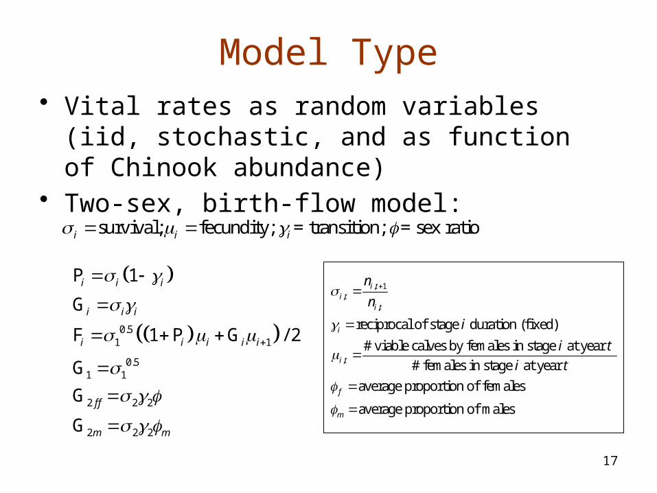
Model Type• Vital rates as random variables (iid, stochastic,

and as function of Chinook abundance)• Two-sex, birth-flow model:

survival; fecundity; = transition; = sex ratioi i i

0.51 1

0.51 1

2 2 2

2 2 2

P 1

G

F 1 P G / 2

G

G

G

i i i

i i i

i i i i i

f f

m m

, 1,

,

,

reciprocal of stage duration (fixed)

# viable calves by females in stage at year

# females in stage at year

average proportion of females

average proportion of mal

i ti t

i t

i

i t

f

m

n

n

i

i t

i t

es

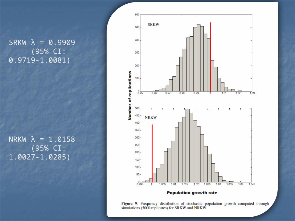
SRKW λ = 0.9909 (95% CI: 0.9719-1.0081)

NRKW λ = 1.0158 (95% CI: 1.0027-1.0285)

19

0%

20%

40%

60%

80%

100%

120%

σ1 σ2 σ3 σ4 σ5 σ6 σ7 µ3 µ4

Vital Rate

CV

(Vita

l Rat

e)

NRKW

SRKW

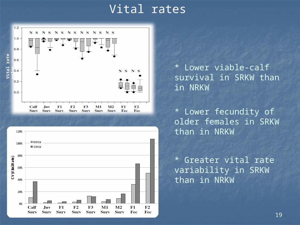
* Lower viable-calf survival in SRKW than in NRKW

* Lower fecundity of older females in SRKW than in NRKW

* Greater vital rate variability in SRKW than in NRKW

Vital ratesV

ital

rat

e va

lue

20

Cumulative difference in vital-rate value (1987-

2011)

21

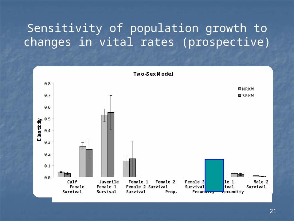
Sensitivity of population growth to changes in vital rates (prospective)

Two-Sex Model

0.0

0.1

0.2

0.3

0.4

0.5

0.6

0.7

0.8

σ1 σ2 σ3 σ4 σ5 σ6 σ7 φ µ3 µ4

Vital Rate

Ela

sti

cit

y

NRKW

SRKW

Calf Juvenile Female 1 Female 2 Female 3 Male 1 Male 2 Female Female 1 Female 2 Survival Survival Survival Survival Survival Survival Survival Prop. Fecundity Fecundity

22

Maximum increase in population growth from maximization of individual vital rates

(1.0 for survival; upper 95% CL for fecundity)

0.000

0.002

0.004

0.006

0.008

0.010

0.012

0.014

0.016

0.018

0.020

0.022

0.024

0.026

0.028

0.030

0.032

0.034

σ1 σ2 σ3 σ4 µ3 µ4

Vital Rate

Max

imu

m P

rop

ort

ion

al In

crea

se in

Lam

bd

a

NRKW

SRKW

Calf Juvenile Female 1 Female 2 Female 1 Female 2

Survival Survival Survival Survival Fecundity Fecundity

Necessary increase to attain U.S. SRKW target population growth rate (2.3% per year)

λ = 1.017

23

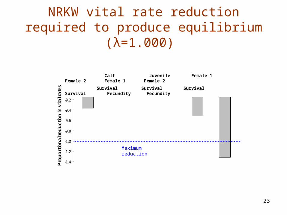
NRKW

-1.4

-1.2

-1.0

-0.8

-0.6

-0.4

-0.2

0.0

σ1 σ2 σ3 σ4 µ3 µ4

Pro

po

rtio

na

l re

du

cti

on

in v

ita

l ra

tes

NRKW vital rate reduction required to produce equilibrium (λ=1.000)

Calf Juvenile Female 1 Female 2 Female 1 Female 2

Survival Survival Survival Survival Fecundity Fecundity

Maximum reduction

24

0%

5%

10%

15%

20%

25%

30%

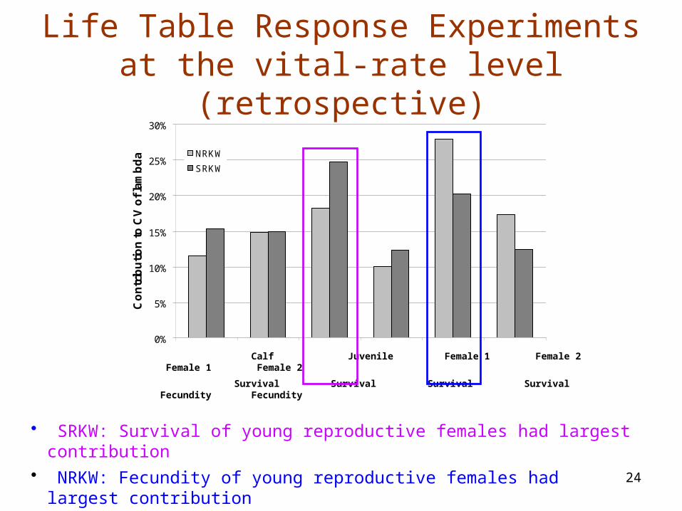
σ1 σ2 σ3 σ4 µ3 µ4

Vital Rate

Co

ntr

ibu

tio

n t

o C

V o

f la

mb

da NRKW

SRKW

Calf Juvenile Female 1 Female 2 Female 1 Female 2

Survival Survival Survival Survival Fecundity Fecundity

• SRKW: Survival of young reproductive females had largest contribution

• NRKW: Fecundity of young reproductive females had largest contribution

Life Table Response Experiments at the vital-rate level (retrospective)

25

Greatest benefits to λ

Avoiding reductions to survival of young reproductive females (Female-1)

Increasing fecundity rates (particularly of Female-1)

26

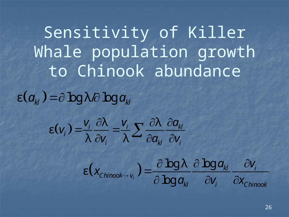
Sensitivity of Killer Whale population growth to Chinook

abundance

ε log λ/ logkl kla a

λ λε

λ λi i kl

ii kl i

v v av

v a v

loglog λε

logi

kl iChinook v

kl i Chinook

a vx

a v x

27

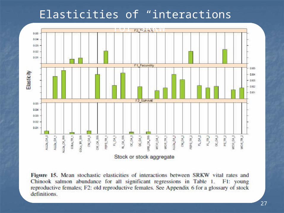
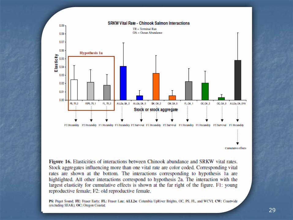
Elasticities of “interactions” for SRKW

28

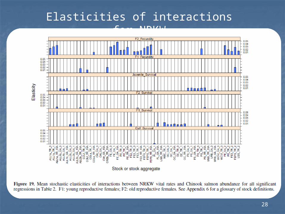
Elasticities of interactions for NRKW

29

30

PVA: selected fishing scenarios (2/12)(elasticities: low sensitivity of killer whale λ to changes in Chinook

abundance)

Recovery Objective for SRKW Maximize Chinook abundance (i.e., minimize fishing

mortality)

Maximize vital rates Whatever occurs first

Response Objective for NRKW Halting population growth (λ = 1.000) Maximize fishing mortality Whatever occurs first

31

32

SRKW under status quo conditions – Population size

33

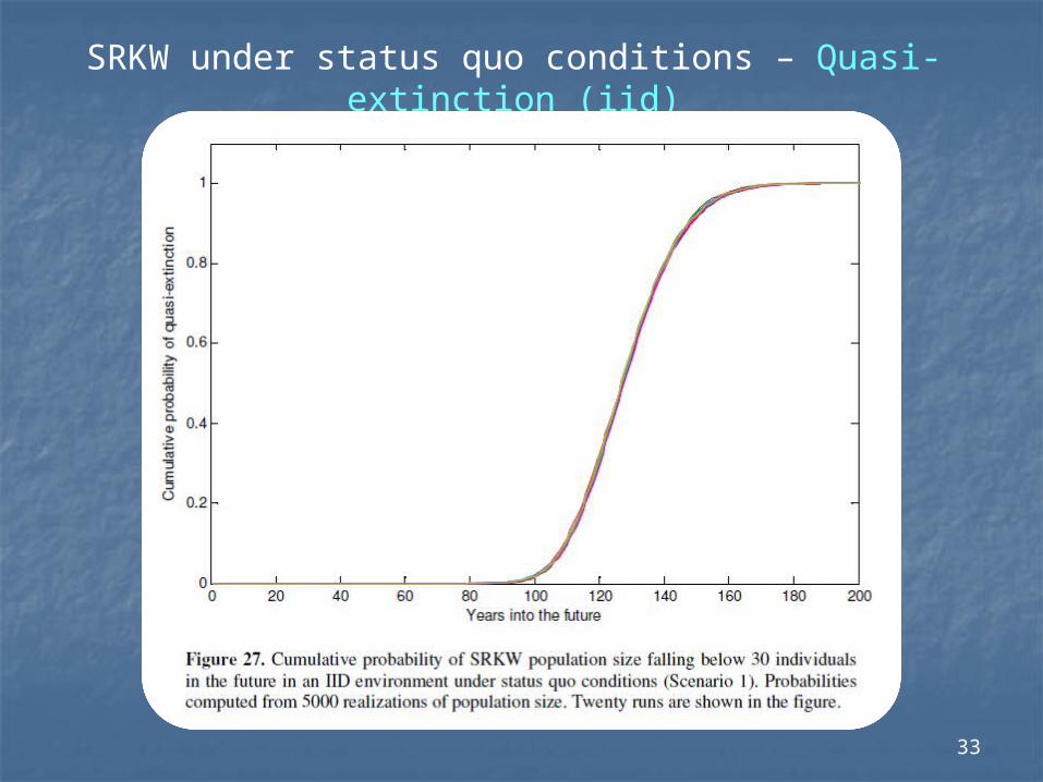
SRKW under status quo conditions – Quasi-extinction (iid)

34

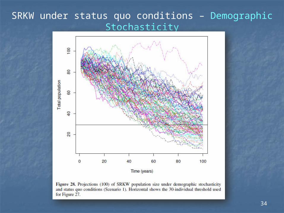
SRKW under status quo conditions – Demographic Stochasticity

35

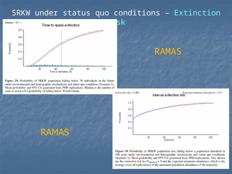
SRKW under status quo conditions – Extinction risk

RAMAS

36

SRKW under Scenario 4 (strongest response) – Population size

Weak hypothesis

37

SRKW under Scenario 4 – Quasi-extinction (iid)

38

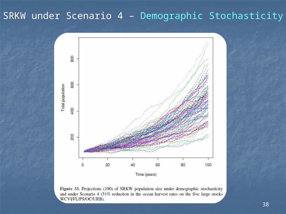
SRKW under Scenario 4 – Demographic Stochasticity

39

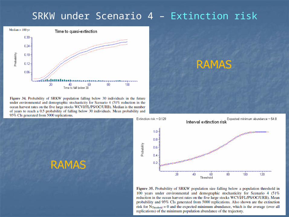
SRKW under Scenario 4 – Extinction risk

40

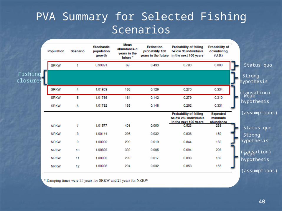
PVA Summary for Selected Fishing Scenarios

Strong hypothesis (causation)

Strong hypothesis (causation)

Fishing closures

Weak hypothesis (assumptions)

Weak hypothesis (assumptions)

Status quo

Status quo

41

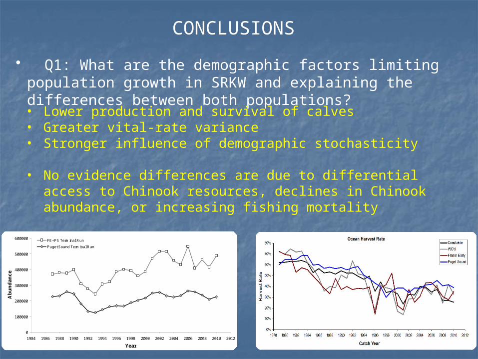
• Q1: What are the demographic factors limiting population growth in SRKW and explaining the differences between both populations?

CONCLUSIONS

• Lower production and survival of calves• Greater vital-rate variance• Stronger influence of demographic stochasticity

• No evidence differences are due to differential access to Chinook resources, declines in Chinook abundance, or increasing fishing mortality

0

100000

200000

300000

400000

500000

600000

1984 1986 1988 1990 1992 1994 1996 1998 2000 2002 2004 2006 2008 2010 2012

Year

Ab

un

da

nc

e

FE+PS Terminal Run

Puget Sound Terminal Run

42

• Q2: What is the influence of Chinook salmon on the population dynamics of both SRKW and NRKW?

CONCLUSIONS

• Numerous interactions between killer whale vital rates & Chinook abundance

• Interactions were weak on statistical & demographic grounds

• Other factors maybe limiting SRKW population growth & probably masking detection of stronger interactions

• Some interactions lent support for causation (Fraser River & Puget Sound)

British Columbia

Washington

50°N 50°N

55°N 55°N

130°W

130°W

N

Kilometres

0 100 200

SE Alaska

43

• Q3: How RKW populations are expected to respond to changes in Chinook fishing mortality?

CONCLUSIONS

• Maximum expected change in population growth resulting from a δ% change in the Chinook abundance of a given stock aggregate never exceeded 0.048*δ in SRKW or 0.046*δ in NRKW

• These low interaction levels could still produce slightly

positive population growth rates in SRKW approximately 50% of the time under extreme reductions to fishing mortality

• It remains a challenge exerting adjustments to ocean harvest rates of specific Chinook stock aggregates in mixed-stock fisheries

44

THANKS!!

QUESTIONS?

Prepared for: BioVeL Workshop “Modeling population response to environmental

change” Amsterdam, March 5-8 2013