Embed Size (px)
Citation preview

1
Rules of Thumb in Real Options Applications
George Y. WangGeorge Y. WangNational Dong-Hwa University
2004 NTU Conference on FinanceDecember 20, 2004

2
Capital Budgeting Practices
0%
20%
40%
60%
80%
Klammer (1972) 29% 30% 39% 35% 3%
Brigham (1975) 70% 78% 48% 74% 18%
Gitman and Forrester (1977) 10% 54% 25% 9% 3%
Oblak and Helm (1980) 14% 60% 14% 10% 2%
Klammer and Walker (1984) 54% 8% 4% 17%
Gilbert and Reichert (1995) 85% 82% 46% 63%
Jog and Srirastava (1995) 85% 82% 46% 63%
Arnold & Hatzopoulos (2000) 80% 81% 56% 70% 31%
Graham and Harvey (2001) 75% 76% 20% 86% 12%
NPVIRR (or Hurdle
Rate)ARR Payback PI Others

3
Capital Budgeting Practices
The literature indicates that NPV, IRR, and payback are top-three frequently used valuation techniques.
Busby and Pitts (1997) and Graham and Harvey (2001) reveal that only a small percentage of firms have formal procedures to appraise real options.

4
MotivationCapital budgeting literature suggests two important facts: first, conventional capital budgeting techniques are shown to have various theoretical shortcomings, yet still have widespread applications in practice; second, real options techniques are considered as relatively sophisticated analysis tools, yet most firms do not make explicit use of real options techniques to evaluate capital investments. This paper aims to bridge the theory-practice gap by translating real options theory into existing capital budgeting practices.

5
Research Purposes
Explore how real options decision criteria can be transformed into equivalent capital budgeting criteria such as NPV, profitability index, hurdle rate, and (discounted) payback. Propose heuristic investment rules in terms of capital budgeting practices to proxy for the inclusion of real options valuation.

6
Modified Capital Budgeting Rules under Real Options (Generalized
Expressions)
NPV
Profitability Index
Payback
Hurdle Rate
Cash Flow Trigger
Discounted Payback
( )NPV V I F V
V
I
V I
ln 1( )
, 0
1 , 0
P
1ln 1
1DP

7
The Comparison between the Modified Investment Rules and
Conventional Rules

8
Stochastic Processes of Interest
0
20
40
60
80
100
120
140
1 11 21 31 41 51 61 71 81 91 101 111 121 131 141 151 161 171 181 191 201
Week
$
GBM Mean Reversion
0
20
40
60
80
100
120
140
1 11 21 31 41 51 61 71 81 91 101 111 121 131 141 151 161 171 181 191 201
Week
$
GBM Mixed1 Mixed2

9
Options, F(V*), and Investment Triggers, V*
GBM
Mixed Diffusion-Jump
Mean Reversion
1( ; ) bF V V AV
1bA V I V
2
1 2 2 2
1 ( ) ( ) 1 2
2 2
r r rb
( ; ) ; ,MRF V V BV G x g
2
2 2 2
1 ( ) 1 2
2 2
r V r V r
2
2x V
2
22
r Vg
2 3( 1) ( 1)( 2)
; , 1( 1) 2! ( 1)( 2) 3!
x xG x g x
g g g g g g
2
2 2 2 2
1 ( ) ( ) 1 2( )
2 2
r r rb
where
2( ; ) bF V V AV
where
where
Pyndick (1991) and Dixit and Pindyck (1994)Pyndick (1991) and Dixit and Pindyck (1994)

10
Real Options in Capital Budgeting (GBM and Mixed Diffusion-Jump)
Profitability Index
Cash Flow Trigger
Hurdle Rate
Payback
Discounted Payback
1
11
1GBM b
1
1
1GBM I Ib
1
1
1GBM b
1
1
1
ln 1( 1)( )
, 0
1 1 , 0
GBM
bb
P
b
1lnDGBM
bP

11
The Option Impact
±=
Modified Rules = Conventional Rules + Option Impact(for PI, Hurdle Rate, and Cash Flow Rules)(for PI, Hurdle Rate, and Cash Flow Rules)
Modified Rules = Conventional Rules – Option Impact(for Payback Rules)(for Payback Rules)

12
Numerical Analysis of the Optimal Triggers under Alternative Processes
100
150
200
250
300
350
0 5% 10% 15% 20% 25% 30% 35% 40%
Volatility
Trig
ger V
alue
GBM or Mixe(λ = 0)
Mixed (λ = 10%)
Mixed (λ = 20%)
Mixed (λ = 30%)
MR (η = 0.02)
MR (η = 0.03)
MR (η = 0.04)
GBM Model
Mixed Diffusion-Jump
Mean Reversion
100, 5%, r 5%I V

13
Findings
The graph suggests that for a set of reasonable parameter values, both mean reversion and competitive arrivals have a significant influence on lowering optimal triggers, indicating that investment in both cases should be launched sooner than the normal GBM case. It seems that mean reversion has a stronger power to induce investment than the competitive arrival effect.

14
The Comparison between the Modified Investment Rules and
Conventional Rules

15
The Cost of Suboptimal Investment Rules under a GBM
0
4
8
12
16
100 120 140 160 180 200 220 240 260 280 300
Arbitrary Trigger ($)
Opt
ion
Val
ue ($
)
ρ =20%, σ =20% ρ =30%, σ =20% ρ =20%, σ =40% ρ =30%, σ =40%
L
H100, 5%, 5%V I r

16
The Cost of Suboptimal Investment Rules under a Mixed Diffusion-Jump
0
4
8
12
16
100 120 140 160 180 200 220 240 260 280 300
Arbitrary Trigger ($)
Opt
ion
Val
ue ($
)
ρ =20%, σ =20%, λ =0.2 ρ =30%, σ =20%, λ =0.2 ρ =20%, σ =40%, λ =0.2
ρ =30%, σ =40%, λ =0.2 ρ =20%, σ =40%, λ =0.4 ρ =20%, σ =40%, λ =0.4
H
L
100, 5%, 5%V I r

17
0
5
10
15
20
25
30
35
100 110 120 130 140 150 160 170 180 190 200
Arbitrary Trigger ($)
Opt
ion
Val
ue ($
)
η =0.03, σ =20% η =0.05, σ =20% η =0.03, σ =40% η =0.05, σ =40%
L H
100, 5%, r 5%V I V
The Cost of Suboptimal Investment Rules under a Mean Reversion

18
Findings
The best investment rule under uncertainty is the optimal investment rule itself.
However, if a simple heuristic decision rule is used to approximate V*, the rule should be as near as possible in order to minimize the opportunity cost of adopting the suboptimal investment policy.

19
The Process of Developing Heuristics
Identify a proper stochastic processConduct base-case analysis to determine target investment ruleConduct regression analysis and sensitivity analysis to identify key determinants and weightsFine-tuning the weightsDetermine heuristic rules
Model Formulation
Regression Analysis
Base Case Analysis
Sensitivity Analysis
Monte Carlo Simulation
3-9 Rule2-10 Rule or
2-10-(-2) Rule
GBM ModelDiffusion-Jump
ModelMean Reversion
Model
4-8 Rule
Adjusting the Weights

20
Optimal Hurdle Rate as a Function of σ and μ under a GBM
17%18%
21%
25%
30%
21%24%
28%
32%
37%
31%33%
36%
41%
46%
41%43%
46%
50%
55%
0%
10%
20%
30%
40%
50%
60%
10% 20% 30% 40% 50%
Volatility
The
Opt
imal
Hur
dle
Rat
e
Discount Rate = 10% Discount Rate = 20% Discount Rate = 30% Discount Rate = 40%
(σ )
(γ*
)
8%

21
Optimal Hurdle Rate as a Function of σ and μ under a Mixed Diffusion-
Jump
29%31%
33%35%
38%
42%41%42%
45%
49%
53%
27%25%
23%21%
0%
10%
20%
30%
40%
50%
60%
10% 20% 30% 40% 50%
Volatility
The
Opt
imal
Hur
dle
Rat
e
Discount Rate = 20% Discount Rate = 30% Discount Rate = 40%
(σ )
(γ*
)
8%, 20%

22
Optimal Hurdle Rate as a Function of σ and μ under a
Mean Reversion
21%23%
25%28%
30%31%34%
37%
40%
43%41%
44%
47%
51%
56%
0%
10%
20%
30%
40%
50%
60%
10% 20% 30% 40% 50%
Volatility
The
Opt
imal
Hur
dle
Rat
e
Discount Rate = 20% Discount Rate = 30% Discount Rate = 40%
(σ )
(γ*
)
100, 0.02V

23
The Sensitivity of Other Capital Budgeting Criteria to σ and μ under
a GBM
4.33
5.24
6.65
8.53
10.88
2.43
1.111.63
1.33
2.001.72
1.04
1.481.291.13
1.02 1.08 1.18 1.311.47
0
2
4
6
8
10
12
10% 20% 30% 40% 50%
Volatility
Equ
ival
ent
Pro
fitab
ility
Ind
ex T
rigge
r
Discount Rate = 10% Discount Rate = 20% Discount Rate = 30% Discount Rate = 40%
(σ )
(Π*
)
10.47
13.30
17.06
21.76
8.65
29.21
13.26
19.60
16.00
24.00
37.85
22.77
32.60
28.28
24.94
47.06
41.89
37.71
34.6032.66
0
5
10
15
20
25
30
35
40
45
50
10% 20% 30% 40% 50%
Volatility
Equ
ival
ent
Cas
h F
low
Trig
ger
Discount Rate = 10% Discount Rate = 20% Discount Rate = 30% Discount Rate = 40%
(σ )
(π*
)
7.09
5.89
4.81
3.91
8.19
3.03
5.90
4.28
5.07
3.60
2.40
3.76
2.743.11
3.48
1.962.18
2.402.602.74
0
1
2
3
4
5
6
7
8
9
10% 20% 30% 40% 50%
Volatility
Equ
ival
ent
Pya
back
Trig
ger
Discount Rate = 10% Discount Rate = 20% Discount Rate = 30% Discount Rate = 40%
(σ )
(P*
)
10.60
8.15
6.23
4.82
13.15
4.41
19.61
7.89
11.55
5.78
3.96
15.39
5.11
6.84
9.71
3.564.51
5.90
8.09
12.18
0
5
10
15
20
25
10% 20% 30% 40% 50%
Volatility
Equ
ival
ent
Dis
coun
edt
Pay
back
Trig
ger
Discount Rate = 10% Discount Rate = 20% Discount Rate = 30% Discount Rate = 40%
(σ )
()
DP

24
The Sensitivity of Other Capital Budgeting Criteria to σ and μ under
a MX Process
1.36
1.53
1.75
2.00
2.28
1.77
1.08
1.38
1.22
1.571.53
1.03
1.37
1.231.12
1.021.08
1.161.27
1.39
0
1
1
2
2
3
10% 20% 30% 40% 50%
Volatility
Equ
ival
ent
Pro
fitab
ility
Ind
ex T
rigge
r
Discount Rate = 10% Discount Rate = 20% Discount Rate = 30% Discount Rate = 40%
(σ )
(Π*
)
3.07 3.50 4.00 4.57
2.72
21.26
12.98
16.5914.65
18.80
33.62
22.74
30.16
27.13
24.60
44.54
40.56
37.16
34.4632.65
0
5
10
15
20
25
30
35
40
45
50
10% 20% 30% 40% 50%
Volatility
Equ
ival
ent
Cas
h F
low
Trig
ger
Discount Rate = 10% Discount Rate = 20% Discount Rate = 30% Discount Rate = 40%
(σ )
(π*
)
16.04
14.87
13.73
12.65
17.15
3.99
6.00
4.925.45
4.43
2.67
3.77
2.943.233.52
2.062.252.442.612.74
0
2
4
6
8
10
12
14
16
18
20
10% 20% 30% 40% 50%
Volatility
Equ
ival
ent
Pay
back
Trig
ger
Discount Rate = 10% Discount Rate = 20% Discount Rate = 30% Discount Rate = 40%
(σ )
(P*
)
52.77
42.36
34.66
28.80
66.58
6.93
21.52
10.7014.25
8.48
4.83
15.58
5.947.57
10.22
3.964.866.178.25
12.23
0
10
20
30
40
50
60
70
10% 20% 30% 40% 50%
Volatility
Equ
ival
ent
Dis
coun
ted
Pay
back
Trig
ger
Discount Rate = 10% Discount Rate = 20% Discount Rate = 30% Discount Rate = 40%
()
DP
(σ )

25
Monte Carlo Simulation
26
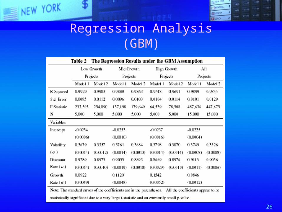
Regression Analysis(GBM)

27
Regression Analysis(Mixed Diffusion-Jump)

28
Regression Analysis(Mean Reversion)

29
Heuristic Investment Rules
Model Formulation
Regression Analysis
Base Case Analysis
Sensitivity Analysis
Monte Carlo Simulation
3-9 Rule2-10 Rule or
2-10-(-2) Rule
GBM ModelDiffusion-Jump
ModelMean Reversion
Model
4-8 Rule
Adjusting the Weights

30
Sensitivity to Growth Rate
Classify five types of projects Project A: high discount rate (μ=35%) and
high volatility (σ=40%) Project B: high discount rate (μ=35%) and
low volatility (σ=10%) Project C: middle discount rate (μ=25%)
and middle volatility (σ=25%) Project D: low discount rate (μ=15%) and
high volatility (σ=10%) Project E: low discount rate (μ=15%) and
low volatility (σ=10%)

31
Sensitivity to Growth RateGBM Model
0%
10%
20%
30%
40%
50%
60%
Growth Rate
Opt
imal
Hur
dle
Rat
e
Project A 44.74% 44.79% 44.84% 44.89% 44.94% 45.00% 45.06% 45.12% 45.19% 45.26% 45.34% 45.42% 45.51% 45.60% 45.70%
Project B 35.64% 35.65% 35.66% 35.66% 35.67% 35.68% 35.68% 35.69% 35.70% 35.71% 35.73% 35.74% 35.75% 35.77% 35.79%
Project C 29.30% 29.35% 29.41% 29.48% 29.55% 29.63% 29.72% 29.81% 29.92% 30.04% 30.18% 30.33% 30.50% 30.70% 30.93%
Project D 26.47% 26.63% 26.81% 27.00% 27.21% 27.43% 27.68% 27.94% 28.23% 28.54% 28.88% 29.25% 29.64% 30.06% 30.52%
Project E 16.00% 16.07% 16.15% 16.26% 16.41% 16.61% 16.89% 17.27% 17.77% 18.39% 19.11% 19.91% 20.76% 21.65% 22.57%
0% 1% 2% 3% 4% 5% 6% 7% 8% 9% 10% 11% 12% 13% 14%
( )
()

32
Sensitivity to Growth RateMixed Diffusion-Jump Model (λ= 20%)
0%
10%
20%
30%
40%
50%
60%
Growth Rate
Opt
imal
Hur
dle
Rat
e
Project A 43.61% 43.59% 43.58% 43.56% 43.54% 43.51% 43.49% 43.45% 43.42% 43.38% 43.33% 43.28% 43.22% 43.16% 43.08%
Project B 35.64% 35.64% 35.65% 35.65% 35.66% 35.66% 35.67% 35.68% 35.69% 35.69% 35.70% 35.71% 35.73% 35.74% 35.75%
Project C 28.78% 28.79% 28.79% 28.79% 28.80% 28.80% 28.79% 28.78% 28.77% 28.75% 28.73% 28.69% 28.65% 28.59% 28.51%
Project D 22.39% 22.22% 22.02% 21.80% 21.55% 21.26% 20.94% 20.57% 20.15% 19.68% 19.13% 18.52% 17.81% 17.00% 16.07%
Project E 15.88% 15.91% 15.94% 15.98% 16.02% 16.06% 16.11% 16.14% 16.17% 16.17% 16.14% 16.06% 15.93% 15.72% 15.41%
0% 1% 2% 3% 4% 5% 6% 7% 8% 9% 10% 11% 12% 13% 14%
()
( )

33
Sensitivity to Growth RateMean Reversion Model
0%
10%
20%
30%
40%
50%
60%
Growth Rate
Opt
imal
Hur
dle
Rat
e
Project A 44.40%44.51%44.62%45.09%45.41%45.45%45.30%45.03%44.69%44.30%43.89%43.48%43.06%42.64%42.22%41.81%
Project B 36.08%36.12%36.14%36.15%36.14%
Project C 29.00%29.29%29.51%29.72%29.75%29.65%29.48%29.26%29.01%28.76%28.50%28.25%27.99%27.74%27.49%27.24%
Project D 26.47%23.93%22.86%21.93%21.08%20.31%19.60%18.96%18.36%17.79%17.27%16.77%16.30%15.85%15.41%15.00%
Project E 16.00%16.07%16.20%16.23%16.19%16.12%16.02%15.91%15.80%15.69%15.57%15.46%15.34%15.23%15.11%15.00%
0% 1% 2% 3% 4% 5% 6% 7% 8% 9% 10% 11% 12% 13% 14% 15%
( )
()

34
4-8 Rule under a GBM
0%
20%
40%
60%
80%
0% 20% 40% 60% 80%
The Heuristic Hurdle Rate
The
Opt
imal
Hur
dle
Rat
e
ρ = 0.9925
0%
20%
40%
60%
80%
0% 20% 40% 60% 80%
The Heuristic Hurdle Rate
The
Opt
imal
Hur
dle
Rat
e
ρ = 0.9900
0%
20%
40%
60%
80%
0% 20% 40% 60% 80%
The Heuristic Hurdle Rate
The
Opt
imal
Hur
dle
Rat
e
ρ = 0.9830
Low-Growth Projects Mid-Growth Projects
High-Growth Projects

35
3-9 Rule under a Mixed Diffusion-Jump
0%
20%
40%
60%
80%
0% 20% 40% 60% 80%
The Heuristic Hurdle Rate
The
Opt
imal
Hur
dle
Rat
e
ρ = 0.9955
0%
20%
40%
60%
80%
0% 20% 40% 60% 80%
The Heuristic Hurdle Rate
The
Opt
imal
Hur
dle
Rat
e
ρ = 0.9909
0%
20%
40%
60%
80%
0% 20% 40% 60% 80%
The Heuristic Hurdle Rate
The
Opt
imal
Hur
dle
Rat
e
ρ = 0.9762
Low-Growth Projects Mid-Growth Projects
High-Growth Projects

36
2-10 Rule and 2-10-(-2) Rule under a Mean Reversion
0%
10%
20%
30%
40%
50%
0% 10% 20% 30% 40% 50%
The Heuristic Hurdle Rate
The
Opt
imal
Hur
dle
Rat
e
ρ = 0.9953
0%
20%
40%
60%
80%
0% 20% 40% 60% 80%
The Heuristic Hurdle Rate
The
Opt
imal
Hur
dle
Rat
e
0.9271
3.76%
( ) 3.37%
0.0023
SD
MSE
2-10 RuleZero-Growth Projects
2-10-(-2) RuleAll Projects
37
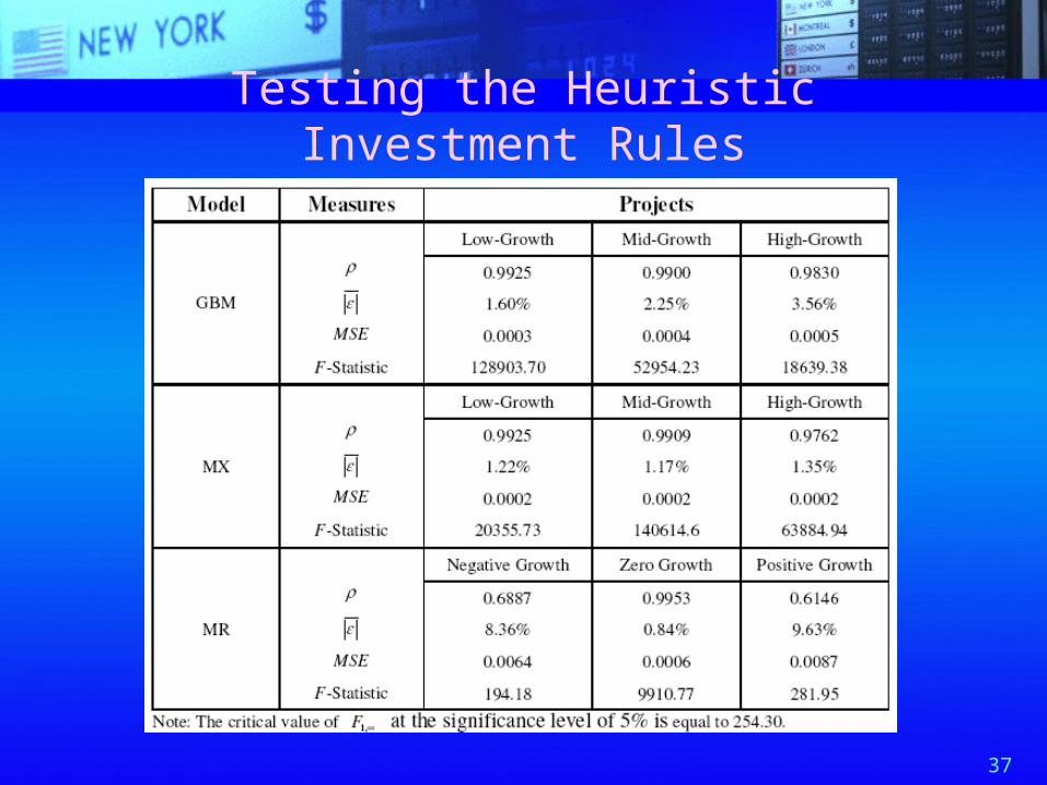
Testing the Heuristic Investment Rules

38
Implications
The heuristic investment rules provide a seemingly accurate approximation to the optimal investment rules by a set of two parameters, volatility and discount rate, under managerial flexibility and uncertainty. Corporate practitioners can apply real options techniques without always carrying out complicated analysis.