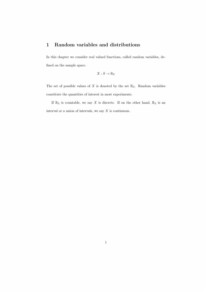
1 Random variables and distributions

In this chapter we consider real valued functions, called random variables, de-

fined on the sample space.

X : S → RX

The set of possible values of X is denoted by the set RX. Random variables

constitute the quantities of interest in most experiments.

If RX is countable, we say X is discrete. If on the other hand, RX is an

interval or a union of intervals, we say X is continuous.

1

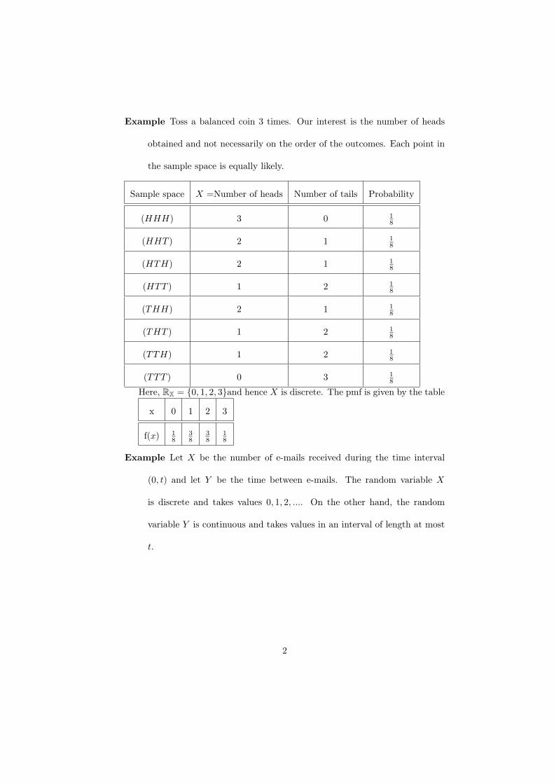
Example Toss a balanced coin 3 times. Our interest is the number of heads

obtained and not necessarily on the order of the outcomes. Each point in

the sample space is equally likely.

Sample space X =Number of heads Number of tails Probability

(HHH) 3 0 18

(HHT ) 2 1 18

(HTH) 2 1 18

(HTT ) 1 2 18

(THH) 2 1 18

(THT ) 1 2 18

(TTH) 1 2 18

(TTT ) 0 3 18

Here, RX = {0, 1, 2, 3}and hence X is discrete. The pmf is given by the table

x 0 1 2 3

f(x) 18

38

38

18

Example Let X be the number of e-mails received during the time interval

(0, t) and let Y be the time between e-mails. The random variable X

is discrete and takes values 0, 1, 2, .... On the other hand, the random

variable Y is continuous and takes values in an interval of length at most

t.

2

Defiinitions

• The probability mass function or probability distribution of the discrete

random variableX is the function f (x) = P (X = x) for all possible values

x. It satisfies the following properties

i) f (x) ≥ 0

ii)∑f (x) = 1

The cumulative distribution function F (x) of a discrete random variable X is

F (x) =∑t≤x

f (t) ,−∞ < x <∞

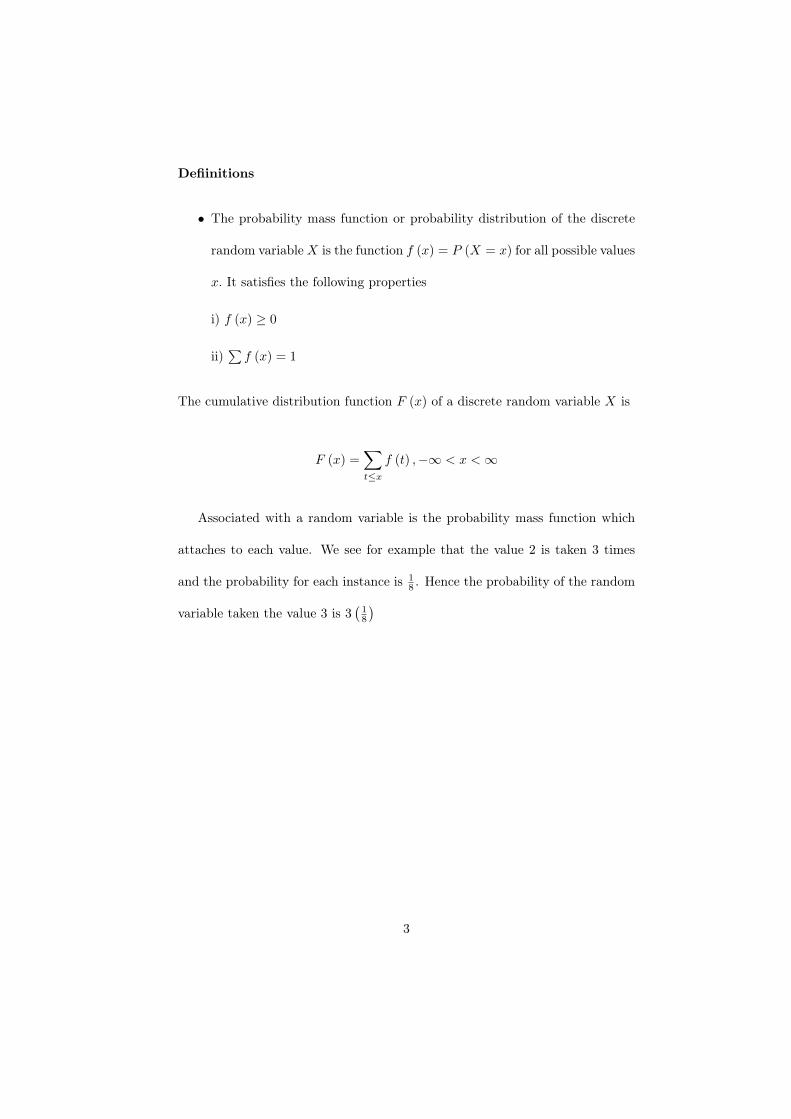
Associated with a random variable is the probability mass function which

attaches to each value. We see for example that the value 2 is taken 3 times

and the probability for each instance is 18 . Hence the probability of the random

variable taken the value 3 is 3(18

)

3

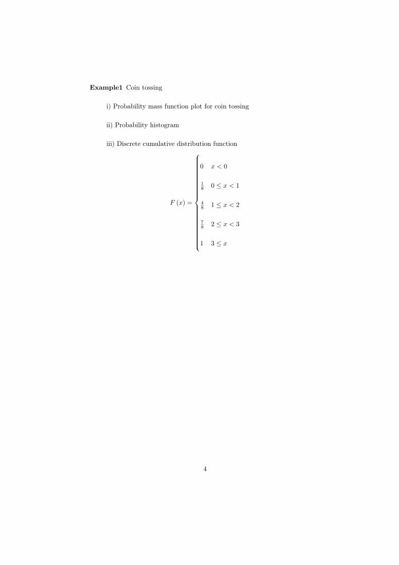
Example1 Coin tossing

i) Probability mass function plot for coin tossing

ii) Probability histogram

iii) Discrete cumulative distribution function

F (x) =

0 x < 0

18 0 ≤ x < 1

48 1 ≤ x < 2

78 2 ≤ x < 3

1 3 ≤ x

4

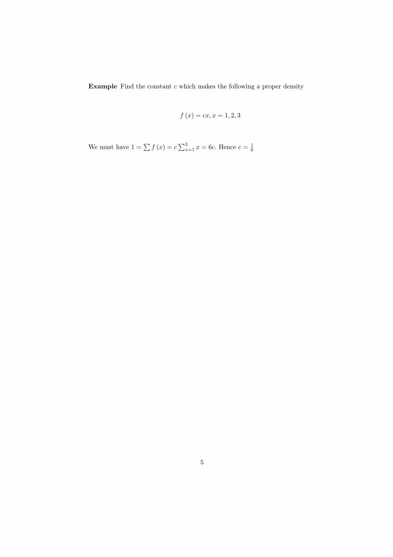
Example Find the constant c which makes the following a proper density

f (x) = cx, x = 1, 2, 3

We must have 1 =∑f (x) = c

∑3x=1 x = 6c. Hence c = 1

6

5

1.1 Continuous probability distributions

If a sample space contains an infinite number of possibilities equal to the number

of points on a line segment, it is called a continuous sample space. For such

a space, probabilities can no longer be assigned to individual values. Instead,

probabilities must be assigned to sub-intervals

P (a < X < b)

Definition The function f (x) is a probability density function for the contin-

uous random variable X defined over the set of real numbers if

i) f (x) ≥ 0, all real x

ii)∫∞−∞ f (x) dx = 1

iii) P (a < X < b) =∫ baf (t) dt

iv) the cumulative distribution function

F (x) = P (X ≤ x) =∫ x

−∞f (t) dt

6

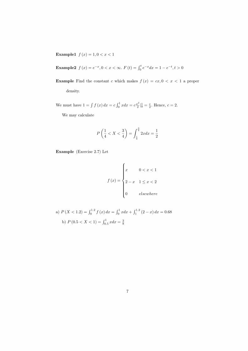
Example1 f (x) = 1, 0 < x < 1

Example2 f (x) = e−x, 0 < x <∞. F (t) =∫ t0e−xdx = 1− e−t, t > 0

Example Find the constant c which makes f (x) = cx, 0 < x < 1 a proper

density.

We must have 1 =∫f (x) dx = c

∫ 1

0xdx = cx

2

2 |10 = c

2 . Hence, c = 2.

We may calculate

P

(1

4< X <

3

4

)=

∫ 34

14

2xdx =1

2

Example (Exercise 2.7) Let

f (x) =

x 0 < x < 1

2− x 1 ≤ x < 2

0 elsewhere

a) P (X < 1.2) =∫ 1.2

0f (x) dx =

∫ 1

0xdx+

∫ 1.2

1(2− x) dx = 0.68

b) P (0.5 < X < 1) =∫ 1

0.5xdx = 3

8

7

1.2 Joint probability distributions

We have situations where more than characteristic is of interest. Suppose we

toss a pair of dice once. The discrete sample space consists of the pairs

{(x, y) : x = 1, ..., 6; y = 1, ..., 6}

where X,Y are the random variables representing the results of the first and

second die respectively. For two electric components in a series connection, we

may be interested in the lifetimes of each.

8

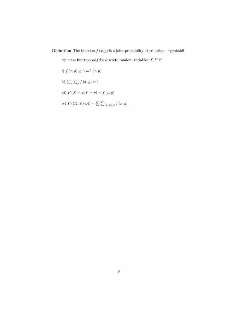
Definition The function f (x, y) is a joint probability distribution or probabil-

ity mass function oϑfthe discrete random variables X,Y if

i) f (x, y) ≥ 0, all (x, y)

ii)∑x

∑y f (x, y) = 1

iii) P (X = x, Y = y) = f (x, y)

iv) P ((X,Y ) εA) =∑∑

(x,y)εA f (x, y)

9

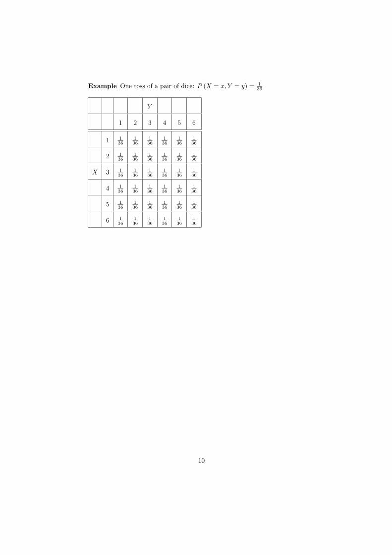
Example One toss of a pair of dice: P (X = x, Y = y) = 136

Y

1 2 3 4 5 6

1 136

136

136

136

136

136

2 136

136

136

136

136

136

X 3 136

136

136

136

136

136

4 136

136

136

136

136

136

5 136

136

136

136

136

136

6 136

136

136

136

136

136

10

Definition The function f (x, y) is a joint probability distribution of the con-

tinuous random variables X,Y if

i) f (x, y) ≥ 0, all (x, y)

ii)∫ ∫

f (x, y) dxdy = 1

iii) P ((X,Y ) εA) =∫ ∫

Af (x, y) dxdy

11

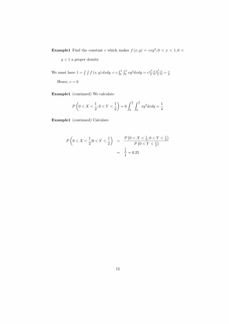
Example1 Find the constant c which makes f (x, y) = cxy2, 0 < x < 1, 0 <

y < 1 a proper density

We must have 1 =∫ ∫

f (x, y) dxdy = c∫ 1

0

∫ 1

0xy2dxdy = cx

2

2 |10y3

3 |10 = c

6

Hence, c = 6

Example1 (continued) We calculate

P

(0 < X <

1

2, 0 < Y <

1

2

)= 6

∫ 12

0

∫ 12

0

xy2dxdy =1

4

Example1 (continued) Calculate

P

(0 < X <

1

2|0 < Y <

1

2

)=

P(0 < X < 1

2 , 0 < Y < 12

)P(0 < Y < 1

2

)=

14

1= 0.25

12

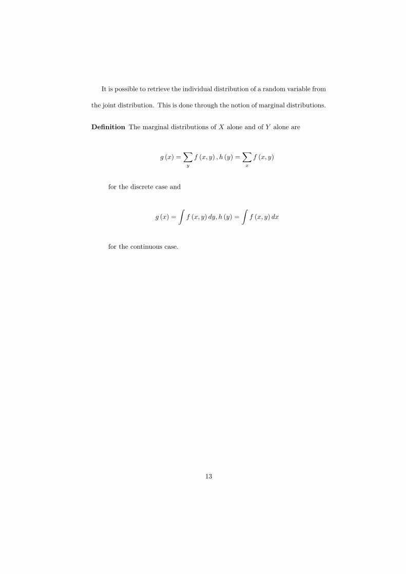
It is possible to retrieve the individual distribution of a random variable from

the joint distribution. This is done through the notion of marginal distributions.

Definition The marginal distributions of X alone and of Y alone are

g (x) =∑y

f (x, y) , h (y) =∑x

f (x, y)

for the discrete case and

g (x) =

∫f (x, y) dy, h (y) =

∫f (x, y) dx

for the continuous case.

13

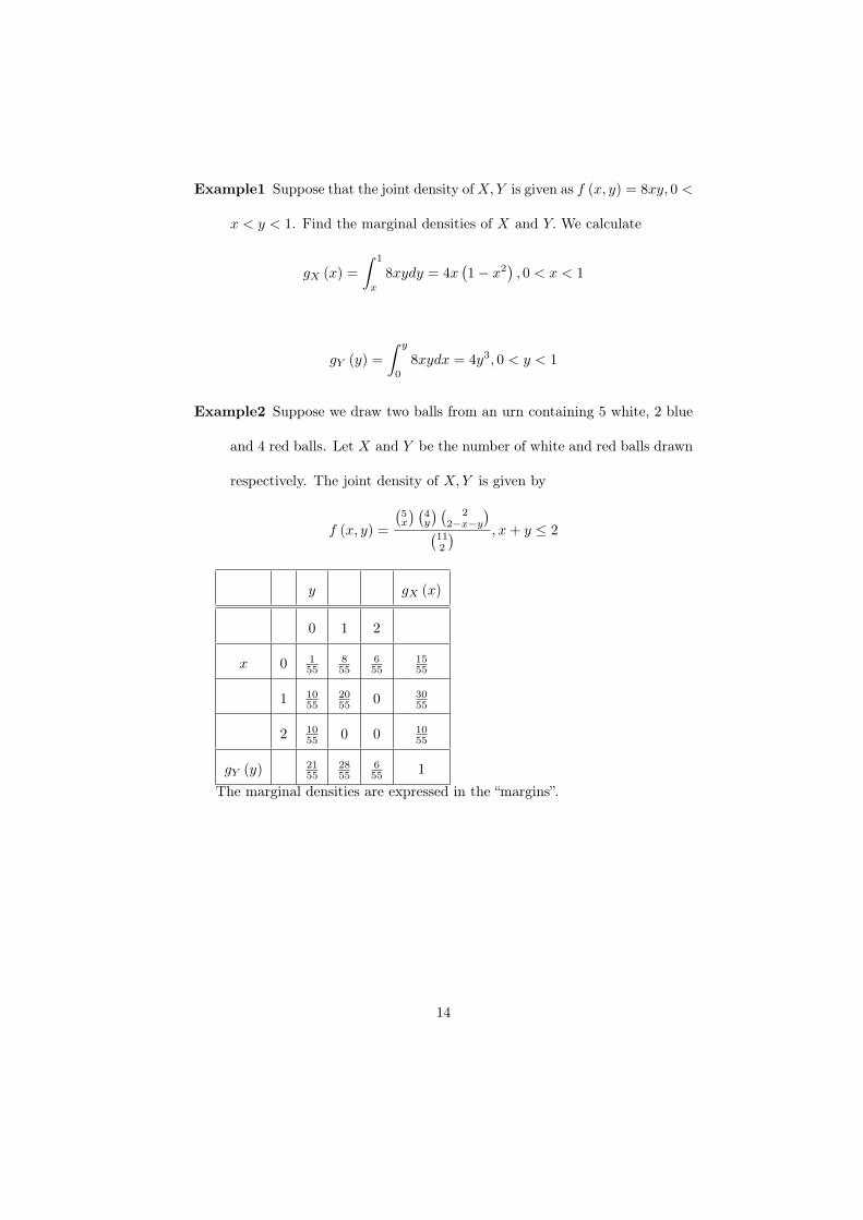
Example1 Suppose that the joint density ofX,Y is given as f (x, y) = 8xy, 0 <

x < y < 1. Find the marginal densities of X and Y. We calculate

gX (x) =

∫ 1

x

8xydy = 4x(1− x2

), 0 < x < 1

gY (y) =

∫ y

0

8xydx = 4y3, 0 < y < 1

Example2 Suppose we draw two balls from an urn containing 5 white, 2 blue

and 4 red balls. Let X and Y be the number of white and red balls drawn

respectively. The joint density of X,Y is given by

f (x, y) =

(5x

) (4y

) (2

2−x−y)(

112

) , x+ y ≤ 2

y gX (x)

0 1 2

x 0 155

855

655

1555

1 1055

2055 0 30

55

2 1055 0 0 10

55

gY (y) 2155

2855

655 1

The marginal densities are expressed in the “margins”.

14

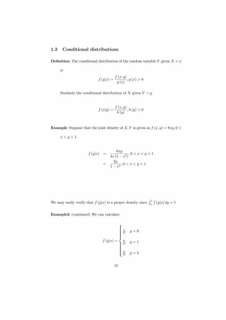
1.3 Conditional distributions

Definition The conditional distribution of the random variable Y given X = x

is

f (y|x) = f (x, y)

g (x), g (x) > 0

Similarly the conditional distribution of X given Y = y

f (x|y) = f (x, y)

h (y), h (y) > 0

Example Suppose that the joint density of X,Y is given as f (x, y) = 8xy, 0 <

x < y < 1.

f (y|x) =8xy

4x (1− x2), 0 < x < y < 1

=2y

1− x2, 0 < x < y < 1

We may easily verify that f (y|x) is a proper density since∫ 1

xf (y|x) dy = 1

Example2 (continued) We can calculate

f (y|x) =

115 y = 0

815 y = 1

615 y = 2

15

The variables are said to be independent if

f (x, y) = g (x)h (y) , all (x, y)

For random variablesX1, ..., Xn with joint density f (x1, ..., xn) and marginals

f1 (x1) , ..., fn (xn) we say they are mutually independent if and only if

f (x1, ..., xn) = f1 (x1) ...fn (xn)

for all tuples (x1, ..., xn) within their range.

Examples In the urn example, X and Y are not independent. Similarly for

the continuous density example.

16

1.4 Properties of random variables

Definition The mean or expected value of a function L of a random variable

X , say L (X) is

µ = E [L (X)] =

∑L (x) f (x) X discrete

∫L (x) f (x) dx X continuous

Definition The mean or expected value of a function L of random variables

X,Y , say L (X,Y ) is

µ = E [L (X,Y )] =

∑L (x, y) f (x, y) X Y, discrete

∫L (x, y) f (x, y) dxdy X Y, continuous

17

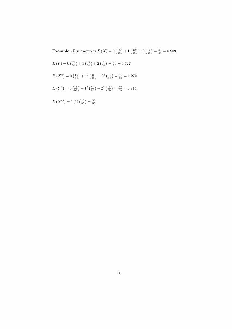
Example (Urn example) E (X) = 0(1555

)+ 1

(3055

)+ 2

(1055

)= 50

55 = 0.909.

E (Y ) = 0(2155

)+ 1

(2855

)+ 2

(655

)= 40

55 = 0.727.

E(X2)= 0

(1555

)+ 12

(3055

)+ 22

(1055

)= 70

55 = 1.272.

E(Y 2)= 0

(1555

)+ 12

(2855

)+ 22

(655

)= 52

55 = 0.945.

E (XY ) = 1 (1)(2055

)= 20

55

18

Definition The covariance of two random variablesX,Y is σXY = E [(X − µX) (Y − µY )] =

E (XY )− µXµY .

Definition The variance of a random variable X is σ2X = E (X − µX)

2=

E (X)2 − µ2

X

Definition The correlation between X,Y is ρ = σXY

σXσY

The variance measures the amount of variation in a random variable taking

into account the weighting given to the values of the random variable. The

correlation measures the “interaction” between the variables. A positive corre-

lation indicates that an increase in X results in an increase in Y . A negative

correlation indicates that an increase inX results in a decrease in Y.

19

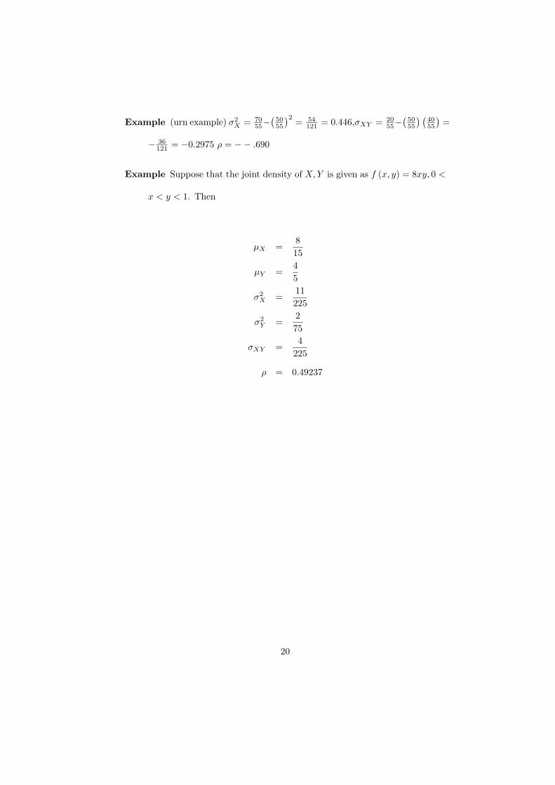
Example (urn example) σ2X = 70

55−(5055

)2= 54

121 = 0.446,σXY = 2055−

(5055

) (4055

)=

− 36121 = −0.2975 ρ = −− .690

Example Suppose that the joint density of X,Y is given as f (x, y) = 8xy, 0 <

x < y < 1. Then

µX =8

15

µY =4

5

σ2X =

11

225

σ2Y =

2

75

σXY =4

225

ρ = 0.49237

20

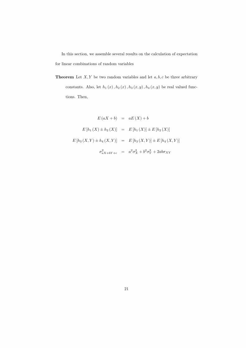
In this section, we assemble several results on the calculation of expectation

for linear combinations of random variables

Theorem Let X,Y be two random variables and let a, b, c be three arbitrary

constants. Also, let h1 (x) , h2 (x) , h3 (x, y) , h4 (x, y) be real valued func-

tions. Then,

E (aX + b) = aE (X) + b

E [h1 (X)± h2 (X)] = E [h1 (X)]± E [h2 (X)]

E [h3 (X,Y )± h4 (X,Y )] = E [h3 (X,Y )]± E [h4 (X,Y )]

σ2aX+bY+c = a2σ2

X + b2σ2Y + 2abσXY

21

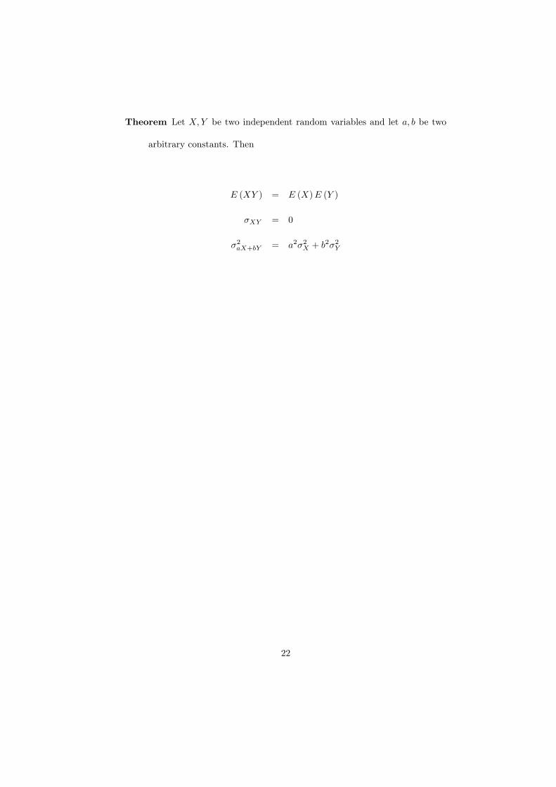
Theorem Let X,Y be two independent random variables and let a, b be two

arbitrary constants. Then

E (XY ) = E (X)E (Y )

σXY = 0

σ2aX+bY = a2σ2

X + b2σ2Y

22

This theorem generalizes to several independent random variables X1, ..., Xn

Theorem Let X1, ..., Xn be random variables and let a1, ..., an be arbitrary

constants. Then

i) E [∑aiXi] =

∑aiE [Xi]

ii)If in addition, X1, ..., Xn are independent random variables

σ2∑aiXi

=∑

a2iσ2Xi

Example Flip a coin with probability of heads p, n times and let Xi = 1 if

we observe heads on the ith toss and Xi = 0, if we observe tails. Assume

the results of the tosses are independent and performed under indentical

conditions. Then, X1, ..., Xn are independent and identically distributed

random variables. The sum,∑Xi represents the number of heads in n

tosses. It follows from the theorem

i) E[1n

∑Xi

]=∑

1nE [Xi] =

1n (np) = p

ii) σ21n

∑Xi

=∑(

1n

)2σ2Xi

= σ2

n = p(1−p)n

The example demonstrates that the average of a set of independent random

variables preserves the mean and importantly reduces the variance by a factor

equal to the size of the sample. .

23