1 Quantitative Approaches to Longitudinal Research Session 2 of RCBN training workshop Longitudinal Research in Education, University of York, 23.1.04

1

Quantitative Approaches to Longitudinal Research

Session 2 of RCBN training workshop Longitudinal Research in Education,

University of York, 23.1.04

Paul Lambert Vernon GayleDept Applied Social Science,

Stirling University

as pl, and: Longitudinal Studies Centre, University of St Andrews

[email protected] [email protected]

http://staff.stir.ac.uk/paul.lambert/

mailto:[email protected]


http://staff.stir.ac.uk/paul.lambert/

2


1. Introduction to and motivations for quantitative longitudinal research

2. Repeated cross-sections

3. Panel datasets 4. Cohort studies

5. Event history datasets 6. Time series analyses

3






4

Introduction to quantitative longitudinal research

i. What constitutes QnLR?

ii. Hypothetical motivations for QnLR

iii. (Perceived) Pragmatic Drawbacks to QnLR

iv. Some advice…

5

i) QnLR in the social sciences

• Data analysis Survey resources – Micro-data (individuals, households, ..)– Macro-data (aggregate summary for year,

country..)

Data analysis is used to give a parsimonious summary of patterns of relations between

variables in the survey dataset

6

i) QnLR in the social sciences

• Qn longitudinal research involves – Focus on time / durations– Focus on change (or stability)– Use of time as control: ‘residual heterogeneity’

• Specific features to QnL– Tends to use ‘large and complex’ secondary

datasets– Particular techniques of data analysis

7

Large & complex social science data

Complexity in: – Multiple points of measurement – Multiple hierarchies of measurement– Array of variables / operationalisations– Relations between / subgroups of cases– Sample collection and weighting

8

ii) Motivations for QnLR

• Time dimension: substantive role of – repeated information over time – durations – changes and stability

• Distinguish age, period and cohort effects• Causality and residual heterogeneity

• Examining multivariate relationships• Representative conclusions• Secondary data analysis positives: other users;

cheap access; range of topics available

9

iii) Drawbacks to QnLR

• Dataset expense: mostly 2ndary; limited access to some data (eg disclosure risk)

• Data analysis: software availability and complexity of some methods

• Unavoidable data management: complex file & variable management requires training and skills of good practice

10

iv) QnLR: Prescriptions for the casual user

• Be aware of range of analytical options – Some research fields get stuck in paradigms

• Technical skills = data management– Put some effort into understanding software

command files (eg STATA or SPSS syntax; ‘dipping into’ windows menus isn’t enough)

• Network– UK QnLR social sciences is quite a small field,

currently quite supportive to each other

11

QnLR: Some research resources

• See reading list for text and internet resources• Training courses in UK – see RCBN site

• A plug for 2 projects at Stirling: Longitudinal Studies Seminar Series

http://www.lss.stir.ac.uk eg workshop St Andrews 27/8 Feb

‘Longitudinal studies in the social sciences’ ESRC funded research methods programme, e-learning &

workshops 2004/5, contact [email protected]

http://www.lss.stir.ac.uk/

http://www.lss.stir.ac.uk/


12






13

Repeated Cross-sections

• By far the most widely used longitudinal analysis in contemporary social sciences

Whole surveys, with same variables, repeated at different time points

and

Same information extracted from different surveys from different time points

14

Illustration: Repeated x-sect dataSurvey Person Person-level Vars

1 1 1 38 1 1

1 2 2 34 2 2

1 3 2 6 - -

2 4 1 45 1 3

2 5 2 41 1 1

3 6 1 20 2 2

3 7 1 25 2 2

3 8 1 20 1 1

N_s=3 N_c=8

15

Some leading repeated cross-section surveys : UK

OPCS Census British Crime Survey

Labour Force Survey British Social Attitudes

New Earnings Survey British Election Studies

Family Expenditure S. Policy Studies (Ethnicity)

General Household Survey

Social Mobility enquires

16

Some leading repeated cross-section surveys : International

European Social Survey PISA

(schoolkid’s aptitudes)

IPUMS census harmonisation

ISSP

LIS/LES (income and employment)

Eurobarometer

17

Repeated cross sections

Easy to communicate & appealing: how things have changed between certain time points

Distinguishes age / period / cohortEasier to analyse – less data management

However.. No other QnL attractions: nature of changers; residual

heterogeneity; causality; durations Hidden complications: are sampling methods, variable

operationalisations really comparable? (don’t overdo: concepts are more often robust than not)

18

Repeated X-sectional analysis

1. Present stats distinctively by time pts– Analytically sound – Tends to be descriptive, limited # vars

2. Time points as an explanatory variable– More complex, requires more assumptions of

data comparability– Can allow a more detailed analysis / models

19

Example 2.1: UK Census• Directly access aggregate statistics from

census reports, books or web, eg:

• Census not that widely used: larger scale surveys often more data and more reliable

Wales: Proportion able to speak Welsh

Year 1891 1981 1991 2001

% 54 19 19 21

20

Eg2.2: UK Labour Force Surveysee syntax examples 2.2

LFS: free download from UK data archive http://www.data-archive.ac.uk/

Same questions asked yearly / quarterly i. Analysis via time groups: output within

survey time pointsii. Analysis by time: pool records and use

time and interactions with time as explanatory variables

http://www.data-archive.ac.uk/

21

Example 2.2i: LFS yearly stats

Percent of UK workers with a higher degree, by employment category and gender (m / f )

Sample size ~35,000 m / 30,000 f each year

1991 1996 2001

Profess. 14.4 19.9 24.9

Non-Prof. 1.3 2.5 3.5

Profess. 11.0 24.4 28.3

Non-Prof 0.6 2.3 3.2

22

Example 2.2ii: LFS and timeLog regression: odds of being a professional from LFS adult workers in 1991,

1996 and 2001

2.383 .000 10.842

-.955 .000 .385

.777 .000 2.174

-.857 .000 .424

.094 .000 1.098

-.195 .000 .823

-.030 .000 .971

-4.232 .000 .015

Higher degree

Female

Age in years (/10)

Age in years squared (/1000)

Time point 1991

Time point 2001

(Time in years)* (Higher Degree)

Constant

aB Sig. Exp(B)

Nagelkere R2=0.11a.

23






24

Panel Datasets

– ‘classic’ longitudinal design

– incorporates ‘follow-up’, ‘repeated measures’, and ‘cohort’

Information collected on the same cases at more than one point in time

25

Panel data in the social sciences

• Large scale studies are ambitious and expensive, normally by major organisations, with efforts made to promote use

• But small scale panels are surprisingly common…

• ‘Balanced’ and ‘Unbalanced’ designs

26

Illustration: Unbalanced panelWave* Person Person-level Vars

1 1 1 38 1 36

1 2 2 34 2 0

1 3 2 6 9 -

2 1 1 39 1 38

2 2 2 35 1 16

3 1 1 40 1 36

3 2 2 36 1 18

3 3 2 8 9 -

N_w=3 N_p=3 *also ‘sweep’, ‘contact’,..

27

Panel data advantages

• Study ‘changers’ – how many of them, what are they like, what caused change

• Control for individuals’ unknown characteristics (‘residual heterogeneity’)

• Develop a full and reliable life history – eg family formation, employment patterns

28

Panel data drawbacks

• Data analysis : can be complex, some methods are advanced / still developing

• Data management : tends to complexity, need training to get on top of

• Dataset access : varies by topics (disclosure risks)

• Attrition (dropout of cases from recontacts)• Long Duration: eg politics of funding

29

Some leading panel surveys : UK

British Household Panel Study (BHPS)

ONS Longitudinal Study (Census 1971->)

British Election Panel Studies

Labour Force Survey rotating panel

School attainment studies (various)

Health and medical progress studies (various)

30

Some leading panel studies : International

European Community Household Panel Study

CHER, PACO, CNEF (individual projects harmonising panels)

Panel Study of Income Dynamics (US)

31

Analytical approaches

i) Study of Transitions / changers – simple methods in any package, eg cross-tab

if changed or not by background influence – but complex data management

ii) Study of durations / life histories – See section 5 ‘event histories’

32

Analytical approachesiii) Panel data models:

Cases i Year t Variables 1 1 1 17 1 1

1 2 1 18 2 1

1 3 1 19 2 -

2 1 1 17 1 3

2 2 1 18 1 1

3 2 2 20 2 2

Yit = ΒXit + … + Є

33

Panel data model types

• Fixed effects - suits smaller samples

• Random effects - ‘variance components’, ‘multilevel model’, suits larger samples

• Growth curves - as VC + time parameters

• Dynamic Lag-effects models - best in theory, but most complex methodologically

Analytically complex and often need advanced or specialist software, eg STATA, S-PLUS, SABRE / GLIM, LIMDEP, MLWIN, …

34

Example 3.1: Panel transitions

• BHPS : annual survey of ~ 10,000 adult householders, plus children interviews

• Attrition very low (though initial non-contacts, & item non-response, are higher)

• Complex recent sample additions

• See many promotional websites..!

35

Aside: BHPS data management

Major BHPS issue is successful data

management

• Good practice: – SPSS or STATA command files to match records

between multiple data files

– Liase with BHPS user support at Essex

– Attend training workshops / see other users’ files, eg http://www.cf.ac.uk/socsi/main/lambertp/stirbhps/

http://www.cf.ac.uk/socsi/main/lambertp/stirbhps/

36

Example 3.1: Panel transitions

Young people’s household circumstance changes by subjective well-being between 1994 and 1995.

BHPS youth panel, 11-14yrs in 1994, row percents. Stays happy

Cheers up

Becomes miserable

Stays miserable

N

HH Stable 54% 19% 10% 18% 499

HH Changes 42% 22% 14% 22% 81

37

Example 3.2: Panel model

BHPS 1994-8: Output from Variance Components Panel model fordeterminants of GHQ scale score (higher = more miserable), by individual

factors for multiple time points per persona

12.69 .168 .000 12.4 13.0

-1.36 .076 .000 -1.5 -1.2

-1.23 .082 .000 -1.4 -1.1

.50 .131 .000 .2 .8

-1.70 .141 .000 -2.0 -1.4

.00 .002 .055 .0 .0

-.07 .076 .356 -.2 .1

.03 .014 .020 .0 .1

ParameterIntercept

Female

In work

Unemployed

FT studying

Age in years

Holds degree ordiploma

Time point

Estimate Std. Error Sig.LowerBound

UpperBound

95% ConfidenceInterval

Variance components : Person level= 46%, individual level = 54%a.

38






39

Cohort Datasets

Information on a group of cases which share a common circumstance, collected

repeatedly as they progress through a life course

– Simple extension of panel dataset

– One of most widely used and intuitive types of repeated contact data (eg ‘7-up’ series)

40

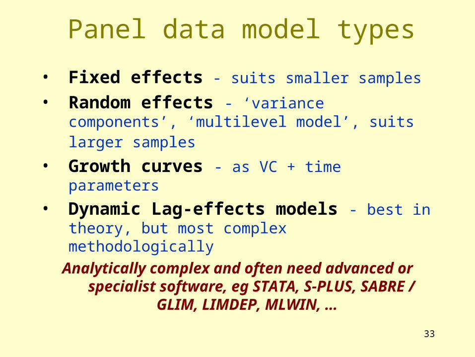
Cohort data in the social sciences

• Circumstances parallel other panel types:Large scale studies ambitious & expensiveSmall scale cohorts still quite common…

Attrition problems often more severeConsiderable study duration problems –

have to wait for generations to age

41

Cohort data advantages

• Study of ‘changers’ a main focus, looking at how group of cases develop after a certain point in time

• Build up a full and reliable life history –often covers a very long span

• May inform on a variety of issues as cohort progresses through lifecourse

42

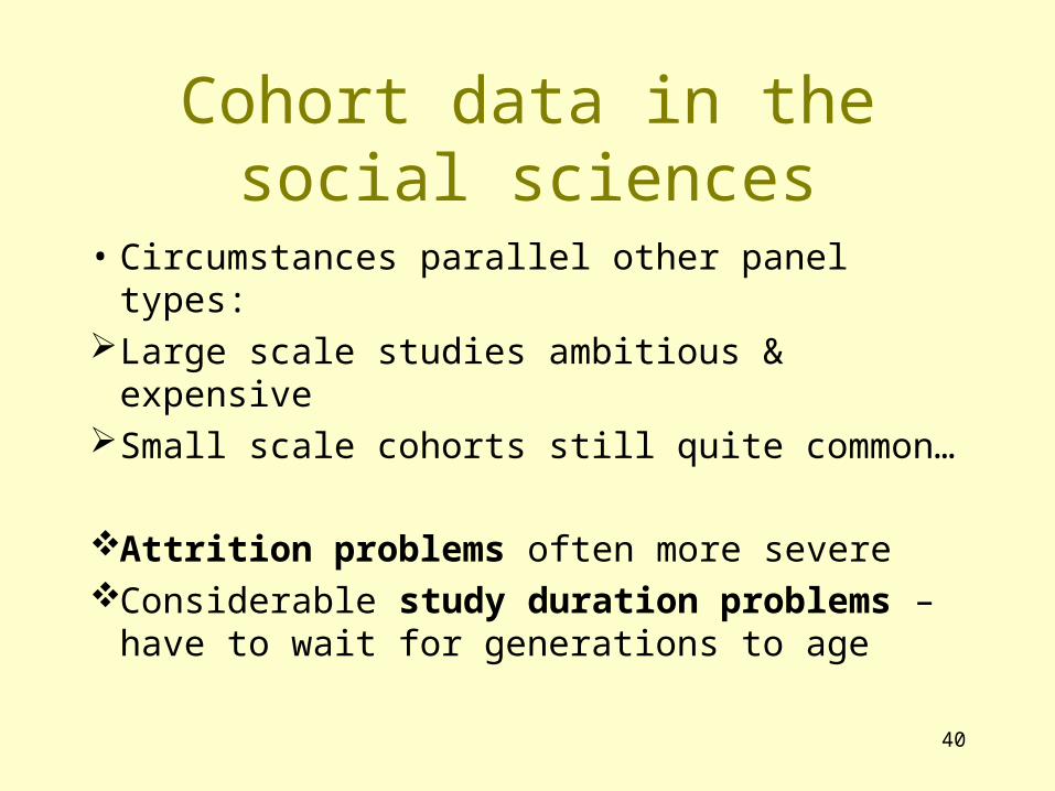
Cohort data drawbacks

• Data analysis & management complexity (less severe than other panels, as generally fewer contact points)

• Attrition problems more severe than panel

• Longer Duration

• Very specific findings – eg only for people of a specific age group

43

Some leading UK cohort surveys

Birth Cohort Studies •1946 National Survey of Health and Development•1958 National Child Development Study•1970 Birth cohort study•2000 Millenium Cohort Study

Youth Cohort Studies (1985 onwards)

Health and medical progress studies (various)

Criminology studies of recidivism (various)

44

Example cohort dataset:

1958 National Child Development Study All women who gave birth in G.B. during the

week of 3-9th March 1958. Approx 17,000 original subjects Several contacts for perinatal mortality studies Subsequent ‘sweeps’ of children at ages 7, 11, 16,

20, 23, 33, 41 12% attrition by 1991 age 33 (this is quite low..)

45

Cohort data analytical approaches

..parallel those of other panel data:

i. Study of transitions / changers

ii. Study of durations / life histories

iii. Panel data models

But focus more on life-course development than shorter term transitions

46

Cohort data analysis example:

“Econometric Analysis of the Demand for Higher Education” (Gayle, Berridge and Davies 2003)

• Youth Cohort Study annual recontacts with teenagers as progress through, then leave, school

• Statistical models: – chances of staying to A-levels,

– then chances of University start, given A-level route

47

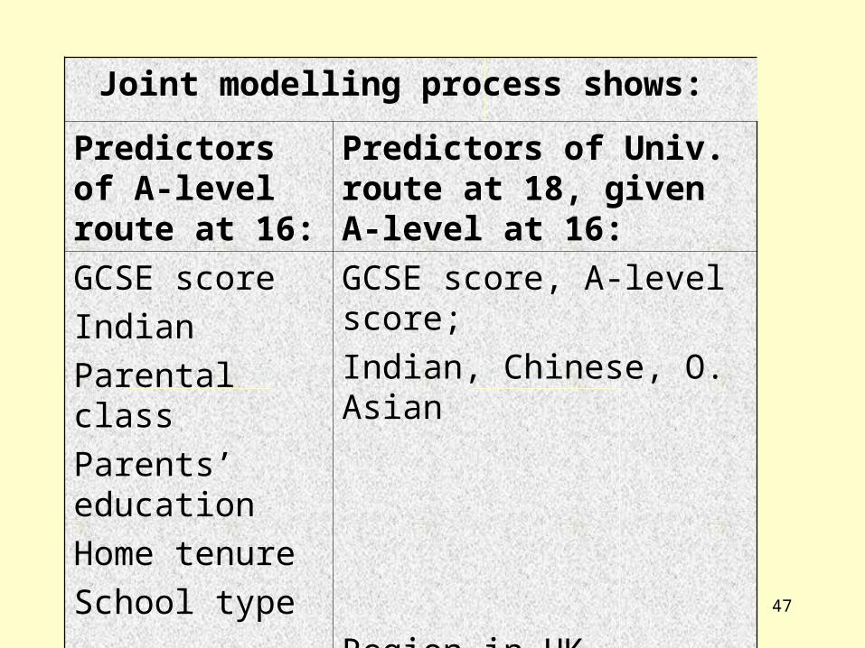
Joint modelling process shows:

Predictors of A-level route at 16:

Predictors of Univ. route at 18, given A-level at 16:

GCSE score

Indian

Parental class

Parents’ education

Home tenure

School type

GCSE score, A-level score;

Indian, Chinese, O. Asian

Region in UK

48






49

Event history data analysis

• Focus shifts to length of time in a ‘state’

• Analyse determinants of time in state

• Alternative data sources: – Panel / cohort (more reliable)– Retrospective (cheaper, but recall errors)

• Aka: ‘Survival data analysis’; ‘Failure time analysis’; ‘hazards’; ‘risks’; ..

50

Social Science event histories:

• Time to labour market transitions

• Time to family formation

• Time to recidivism

Comment: Data analysis techniques relatively new, and aren’t suited to complex variates

Many event history applications have used quite simplistic variable operationalisations

51

Event histories differ:

• In form of dataset (cases are spells in time, not individuals)

Some complex data management issues

• In types of analytical methodMany techniques are new or rare, and

specialist software may be needed

52

Key to event histories is ‘state space’ Episodes within state space : Lifetime work histories for 3 adults born 1935 State space Person 1 FT work PT work Not in work Person 2 FT work PT work Not in work Person 3 FT work PT work Not in work 1950 1960 1970 1980 1990 2000

53

Illustration of a continuous time retrospective dataset Case Person Start

time End time

Duration Origin State

Destination state

{Other vars, person/state}

1 1 1 158 157 1 (FT) 3 (NW) 2 1 158 170 12 3 (NW) 3(NW) 3 2 1 22 21 3 (NW) 1 (FT) 4 2 22 106 84 1 (FT) 3 (NW) 5 2 106 149 43 3 (NW) 2 (PT) 6 2 149 170 21 2 (PT) 2 (PT) 7 3 1 10 9 1 (FT) 2 (PT) . . . . . . .

54

Illustration of a discrete time retrospective dataset Case Person Discrete

Time Approx real time

State End of state

{Other person, state, or time unit level variables}

1 1 1 5 1 FT 0 2 1 2 20 1 FT 0 3 1 3 35 1 FT 0 4 1 4 50 1 FT 0 5 1 5 65 1 FT 0 6 1 6 80 1 FT 0 7 1 7 95 1 FT 0 8 1 8 110 1 FT 0 9 1 9 125 1 FT 0 10 1 10 140 1 FT 1 11 1 11 155 3 NW 0 12 1 12 170 3 NW 1 13 2 1 5 3 NW 0 14 2 2 20 3 NW 1 15 2 3 35 1 FT 0 16 2 4 50 1 FT 1 . . . . . .

55

Event history data permutations

• Single state single episode– Eg Duration in first post-school job till end

• Single episode competing risks– Eg Duration in job until promotion / retire / unemp.

• Multi-state multi-episode– Eg adult working life histories

• Time varying covariates– Eg changes in family circumstances as influence on

employment durations

56

Some UK event history datasets

British Household Panel Study (see separate ‘combined life history’ files)

National Birth Cohort Studies

Family and Working Lives Survey

Social Change and Economic Life Initiative

Youth Cohort Studies

57

Event history analysis software

SPSS – very limited analysis options

STATA – wide range of pre-prepared methods

SAS – as STATA

S-Plus/R – vast capacity but non-introductory

GLIM / SABRE – some unique options

TDA – simple but powerful freeware

MLwiN; lEM; {others} – small packages targeted at specific analysis situations

58

Types of Event History Analysis

i. Descriptive: compare times to event by different groups (eg survival plots)

ii. Modelling: variations of Cox’s Regression models, which allow for particular conditions of event history data structures

• Type of data permutations influences analysis – only simple data is easily used!

59

Eg 5.1 : Mean durations by states

46107141679953328541605658161 172127711862843520870194515516442N =

BHPS first job durations by EGP class200

100

0

Male

Female

60

Eg 5.1 : Kaplan-Meir survival

BHPS males 1st job KM

duration in months

7006005004003002001000-100

Cu

m S

urv

iva

l

1.2

1.0

.8

.6

.4

.2

0.0

-.2

agricultural w k

semi,unskilled

skilled manual

foreman,technicians

farmers

sml props w /o

sml props w /e

personal service

routine non-mnl

service class,lo

service class,hi

61

Eg 5.2: Cox’s regression

Cox regression estimates: risks of quicker exit from firstemployment state of BHPS adults

.194 .081 .017

-.617 .179 .001

-.062 .003 .000

.000 .000 .000

-.013 .001 .000

.214 .109 .049

-.003 .002 .061

.000 .004 .897

.006 .001 .000

Female

Self-employed

Age in 1990

Age in 1990 squared

Hope-Goldthorpe scale

Female*self-employed

Female* HG scale

Self-employed*HG scale

Female*Age in 1990

B SE Sig.

62






63

Time series data

Statistical summary of one particular concept, collected at repeated time points from one or

more subjects

Examples:• Unemployment rates by year in UK• University entrance rates by year by country

64

Time Series Analysis

i) Descriptive analyses

– charts / text commentaries on values by time periods and different groups

– Widely used in social science research – But exactly equivalent to repeated cross-

sectional descriptives.

65

Time Series Analysis

ii) Time Series statistical models

– Advanced methods of modelling data analysis are possible, require specialist stats packages

– Main feature : many measurement points and few cases

– Major area in business / economics, but largely unused in other social sciences

66

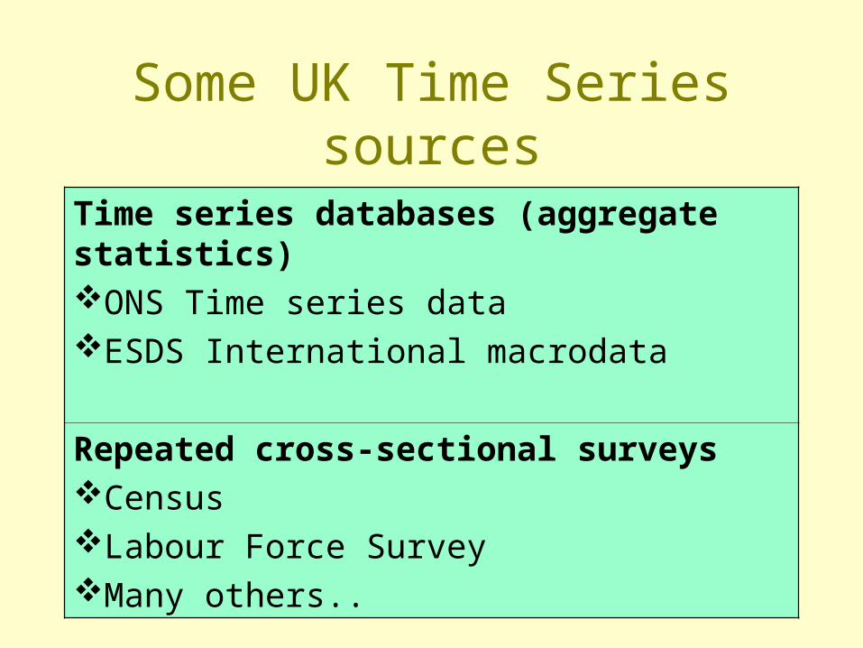
Some UK Time Series sources

Time series databases (aggregate statistics) ONS Time series data ESDS International macrodata

Repeated cross-sectional surveysCensusLabour Force SurveyMany others..

67

….Phew!





68

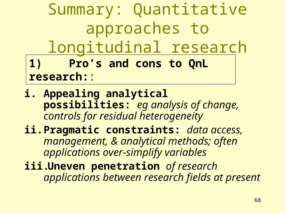
Summary: Quantitative approaches to longitudinal research

i. Appealing analytical possibilities: eg analysis of change, controls for residual heterogeneity

ii. Pragmatic constraints: data access, management, & analytical methods; often applications over-simplify variables

iii. Uneven penetration of research applications between research fields at present

1) Pro’s and cons to QnL research::

69


i. Don’t have to be an expert: Qn longitudinal research influential to social sciences – should be able to understand / critique even if not a practitioner

ii. Understand data collection process and retain sociological background

iii. Make better research proposals!

2) Importance of knowing the research field:

70


i. Needs a bit of effort: learn software, data management practice – workshops and training facilities available

ii. Remain sociologically driven: ‘methodolatry’ widespread in QnL, applications ‘forced’ into desired techniques; often simpler techniques make for the more popular & influential reports

iii. Learn by doing (..try the syntax examples..)

3) Undertaking QnL research::

71

See reading list / internet resources for further information

Documents

1 Quantitative Approaches to Longitudinal Research Session 2 of RCBN training workshop Longitudinal Research in Education, University of York, 23.1.04