1

Psych 5510/6510

Chapter 12

Factorial ANOVA: Models with Multiple Categorical Predictors and Product Terms.

Spring, 2009

2

Factorial Designs

Designs with ‘q’ number of independent variables, each having two or more levels (i.e. each IV has two or more groups), combined in such a way that every level of one independent variable is combined with every level of the other independent variables.

3

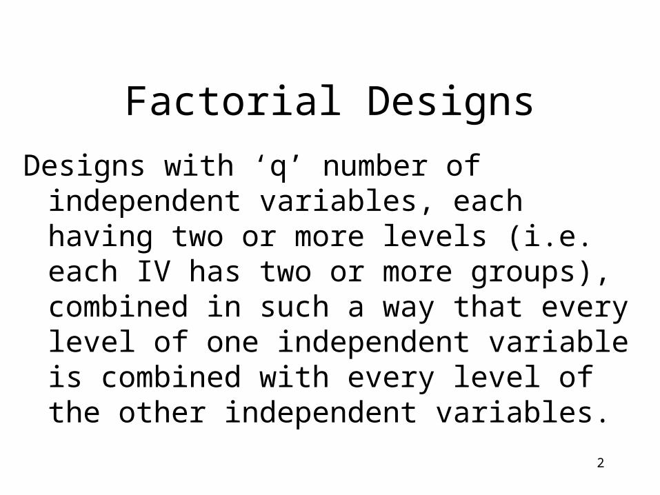
Our example

Independent Variable A: Type of DrugA1: Drug A

A2: Drug B

A3: Placebo

‘a’ = number of levels of A = 3

Independent Variable B: EnzymeB1: With Enzyme

B2: Without Enzyme

‘b’ = number of levels of B = 2

Dependent Variable = Mood

4

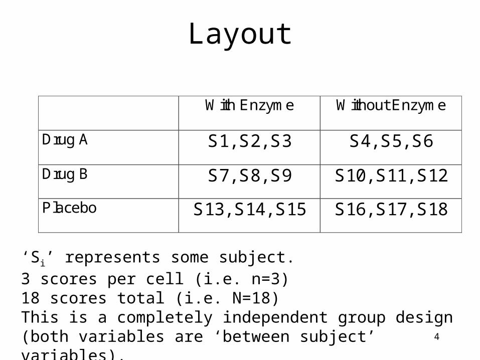
Layout

With Enzyme Without Enzyme

Drug A S1, S2, S3 S4, S5, S6

Drug B S7, S8, S9 S10, S11, S12

Placebo S13, S14, S15 S16, S17, S18

‘Si’ represents some subject.3 scores per cell (i.e. n=3)18 scores total (i.e. N=18)This is a completely independent group design (both variables are ‘between subject’ variables).

5

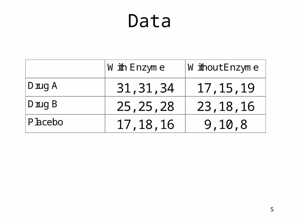
Data

With Enzyme Without Enzyme

Drug A 31, 31, 34 17, 15, 19 Drug B 25, 25, 28 23, 18, 16 Placebo 17, 18, 16 9, 10, 8

6

Means W i t h E n z y m e

( b 1 ) W i t h o u t E n z y m e ( b 2 )

R o w m e a n s

D r u g A ( a 1 )

32Y a1b1 17Y a1b2 5.24Y Drug_A D r u g B ( a 2 )

26Y a2b1 19Y a2b2 5.22Y Drug_B P l a c e b o ( a 3 )

17Y a3b1 9Y 23 ba 13Y Placebo C o l u m n m e a n s

25Y With_E 15Y Without_E

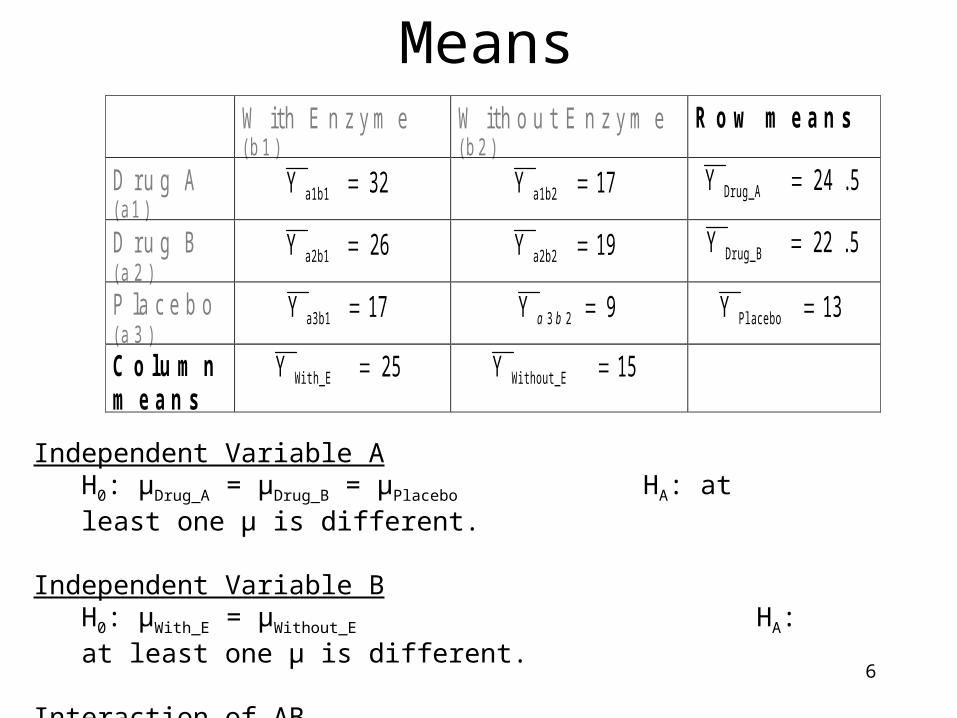
Independent Variable AH0: μDrug_A = μDrug_B = μPlacebo HA: at least one μ is different.

Independent Variable BH0: μWith_E = μWithout_E HA: at least one μ is different.

Interaction of ABH0: A and B do not interact HA: A and B interact

7

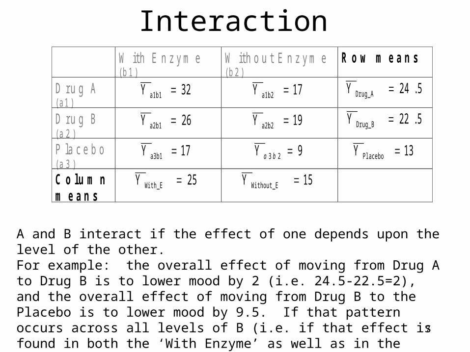
Interaction W i t h E n z y m e

( b 1 ) W i t h o u t E n z y m e ( b 2 )

R o w m e a n s

D r u g A ( a 1 )

32Y a1b1 17Y a1b2 5.24Y Drug_A D r u g B ( a 2 )

26Y a2b1 19Y a2b2 5.22Y Drug_B P l a c e b o ( a 3 )

17Y a3b1 9Y 23 ba 13Y Placebo C o l u m n m e a n s

25Y With_E 15Y Without_E

A and B interact if the effect of one depends upon the level of the other.For example: the overall effect of moving from Drug A to Drug B is to lower mood by 2 (i.e. 24.5-22.5=2), and the overall effect of moving from Drug B to the Placebo is to lower mood by 9.5. If that pattern occurs across all levels of B (i.e. if that effect is found in both the ‘With Enzyme’ as well as in the ‘Without Enzyme’ groups) then the two variables DO NOT interact.

8

Interaction W i t h E n z y m e

( b 1 ) W i t h o u t E n z y m e ( b 2 )

R o w m e a n s

D r u g A ( a 1 )

32Y a1b1 17Y a1b2 5.24Y Drug_A D r u g B ( a 2 )

26Y a2b1 19Y a2b2 5.22Y Drug_B P l a c e b o ( a 3 )

17Y a3b1 9Y 23 ba 13Y Placebo C o l u m n m e a n s

25Y With_E 15Y Without_E

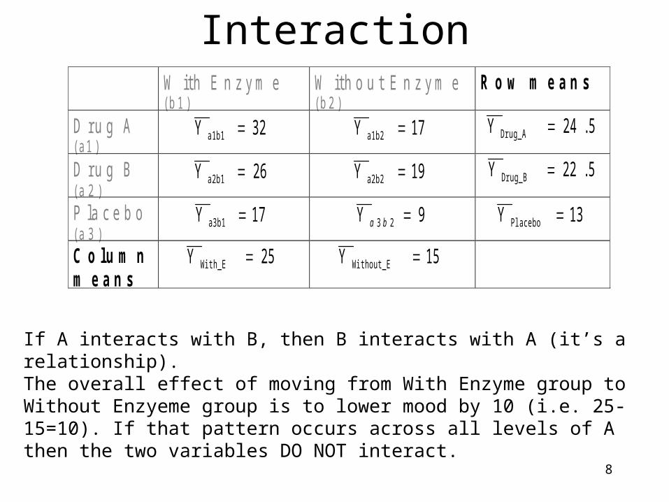
If A interacts with B, then B interacts with A (it’s a relationship).The overall effect of moving from With Enzyme group to Without Enzyeme group is to lower mood by 10 (i.e. 25-15=10). If that pattern occurs across all levels of A then the two variables DO NOT interact.

9

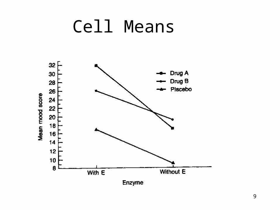
Cell Means

10

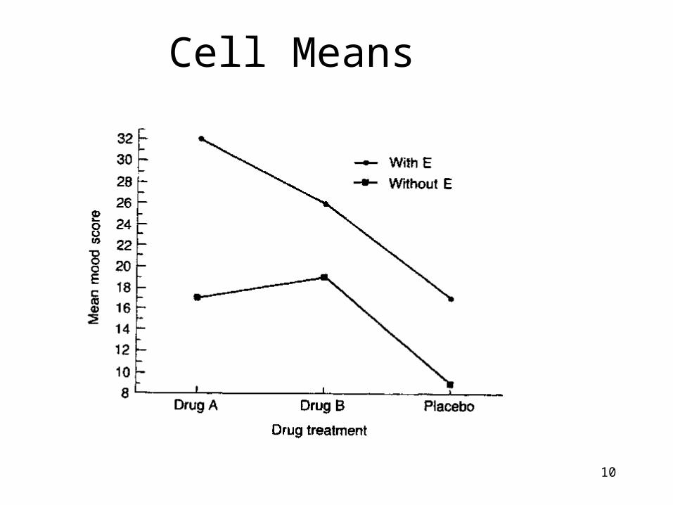
Cell Means

11

Traditional ANOVA Summary Table

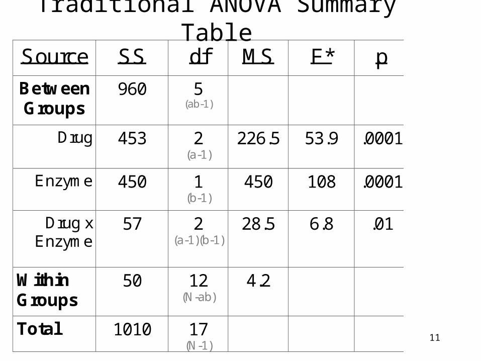
Source SS df MS F* p

Between Groups

960 5 (ab-1)

Drug 453 2 (a-1)

226.5 53.9 .0001

Enzyme 450 1 (b-1)

450 108 .0001

Drug x Enzyme

57 2 (a-1)(b-1)

28.5 6.8 .01

Within Groups

50 12 (N-ab)

4.2

Total 1010 17 (N-1)

12

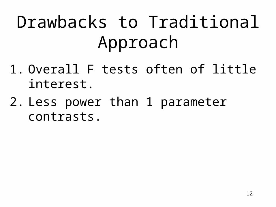
Drawbacks to Traditional Approach

1. Overall F tests often of little interest.

2. Less power than 1 parameter contrasts.

13

Book’s Approach: Setting up Contrast Codes

Drug A With E

Drug B With E

Placebo With E

Drug A Without E

Drug B Without E

Placebo Without E

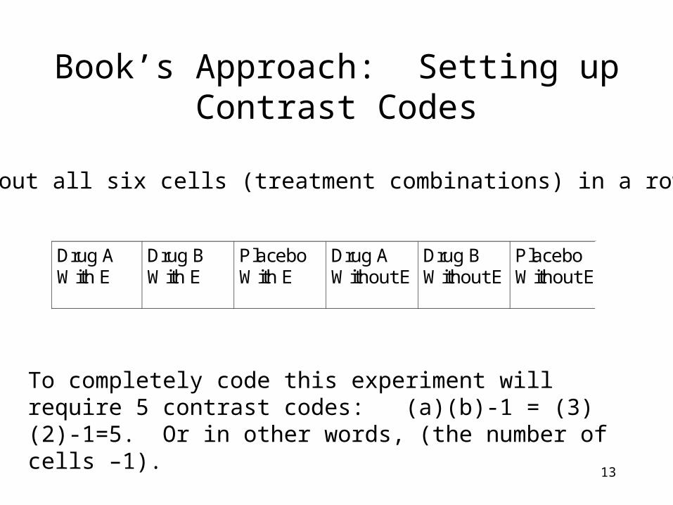
Layout all six cells (treatment combinations) in a row.

To completely code this experiment will require 5 contrast codes: (a)(b)-1 = (3)(2)-1=5. Or in other words, (the number of cells –1).

14

Generating codes

Begin by creating a complete set of contrast codes for each independent variable.

15

IV: Type of Drug

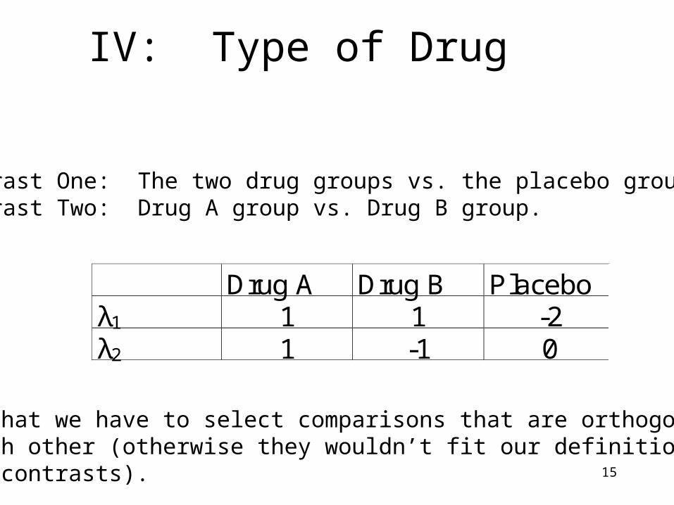
Drug A Drug B Placebo λ1 1 1 -2 λ2 1 -1 0

Contrast One: The two drug groups vs. the placebo groupContrast Two: Drug A group vs. Drug B group.

Note that we have to select comparisons that are orthogonalto each other (otherwise they wouldn’t fit our definition ofbeing contrasts).

16

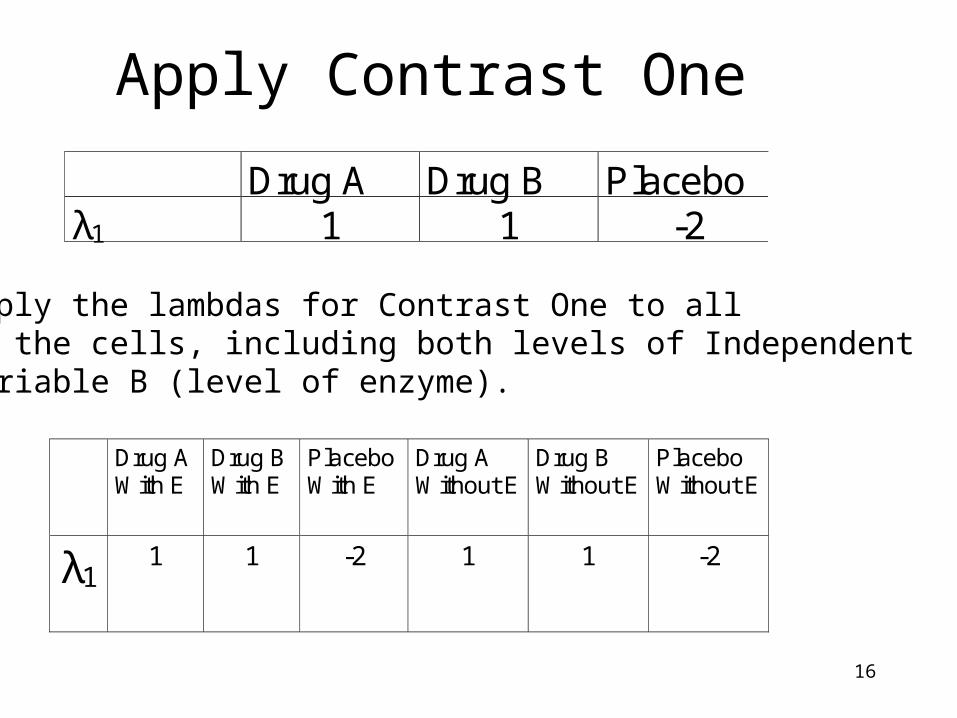
Apply Contrast One

Apply the lambdas for Contrast One to allof the cells, including both levels of Independent Variable B (level of enzyme).

Drug A With E

Drug B With E

Placebo With E

Drug A Without E

Drug B Without E

Placebo Without E

λ1 1 1 -2 1 1 -2

Drug A Drug B Placebo λ1 1 1 -2

17

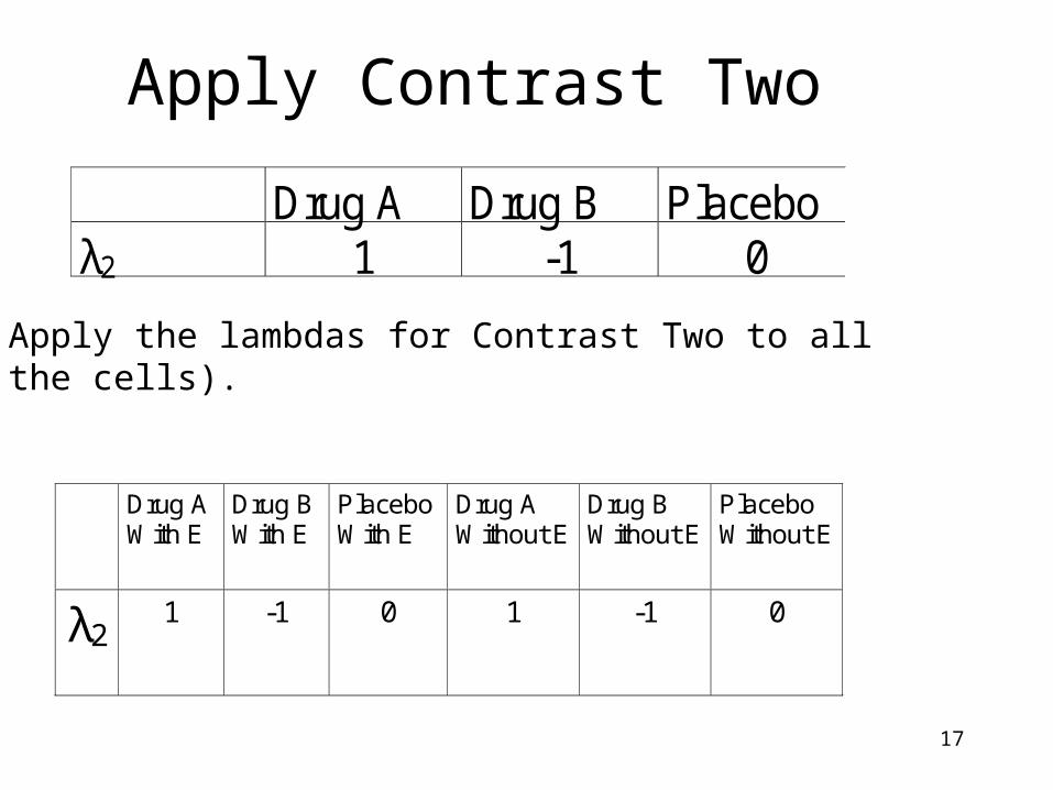
Apply Contrast Two

Apply the lambdas for Contrast Two to allthe cells).

Drug A With E

Drug B With E

Placebo With E

Drug A Without E

Drug B Without E

Placebo Without E

λ2 1 -1 0 1 -1 0

Drug A Drug B Placebo λ2 1 -1 0

18

Contrasts So Far

Drug A With E

Drug B With E

Placebo With E

Drug A Without E

Drug B Without E

Placebo Without E

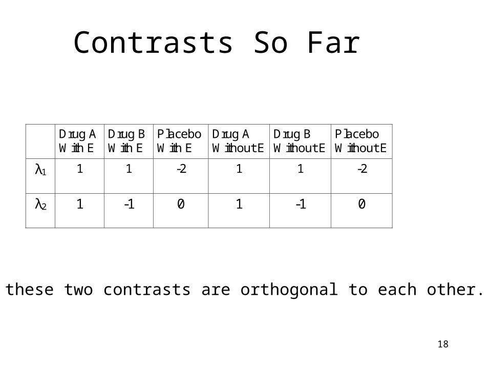
λ1 1 1 -2 1 1 -2

λ2 1 -1 0 1 -1 0

Note these two contrasts are orthogonal to each other.

19

IV: Level of Enzyme

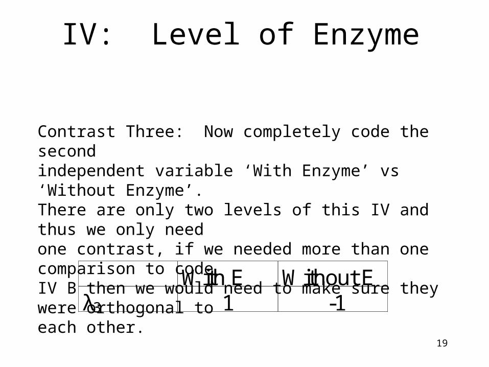
With E Without E λ3 1 -1

Contrast Three: Now completely code the secondindependent variable ‘With Enzyme’ vs ‘Without Enzyme’.There are only two levels of this IV and thus we only needone contrast, if we needed more than one comparison to codeIV B then we would need to make sure they were orthogonal toeach other.

20

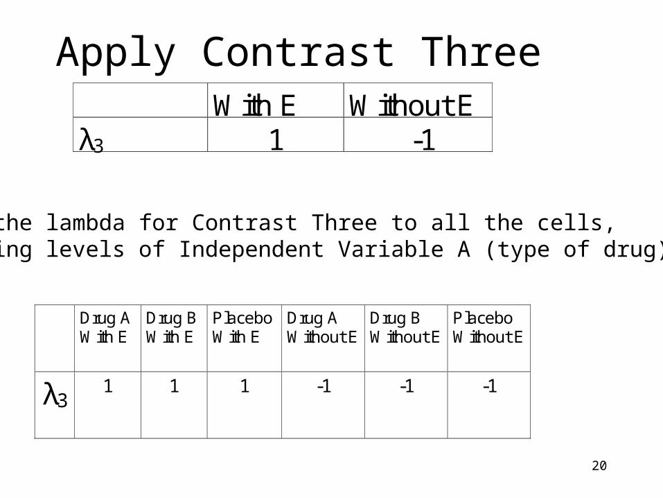
Apply Contrast Three

Apply the lambda for Contrast Three to all the cells,including levels of Independent Variable A (type of drug).

Drug A With E

Drug B With E

Placebo With E

Drug A Without E

Drug B Without E

Placebo Without E

λ3 1 1 1 -1 -1 -1

With E Without E λ3 1 -1

21

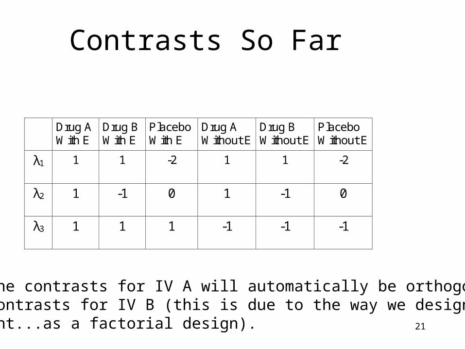
Contrasts So Far

Drug A With E

Drug B With E

Placebo With E

Drug A Without E

Drug B Without E

Placebo Without E

λ1 1 1 -2 1 1 -2

λ2 1 -1 0 1 -1 0

λ3 1 1 1 -1 -1 -1

Note: the contrasts for IV A will automatically be orthogonalto the contrasts for IV B (this is due to the way we designed theexperiment...as a factorial design).

22

Interaction of Type of Drug and Level of Enzyme

Remember we should end up with 5 contrasts, so far we have come up with 3. The final two contrasts will cover the interaction of our two independent variables.

To generate interaction contrast codes multiply each contrast in one IV by each contrast in the other IV.

23

The Interaction Contrasts

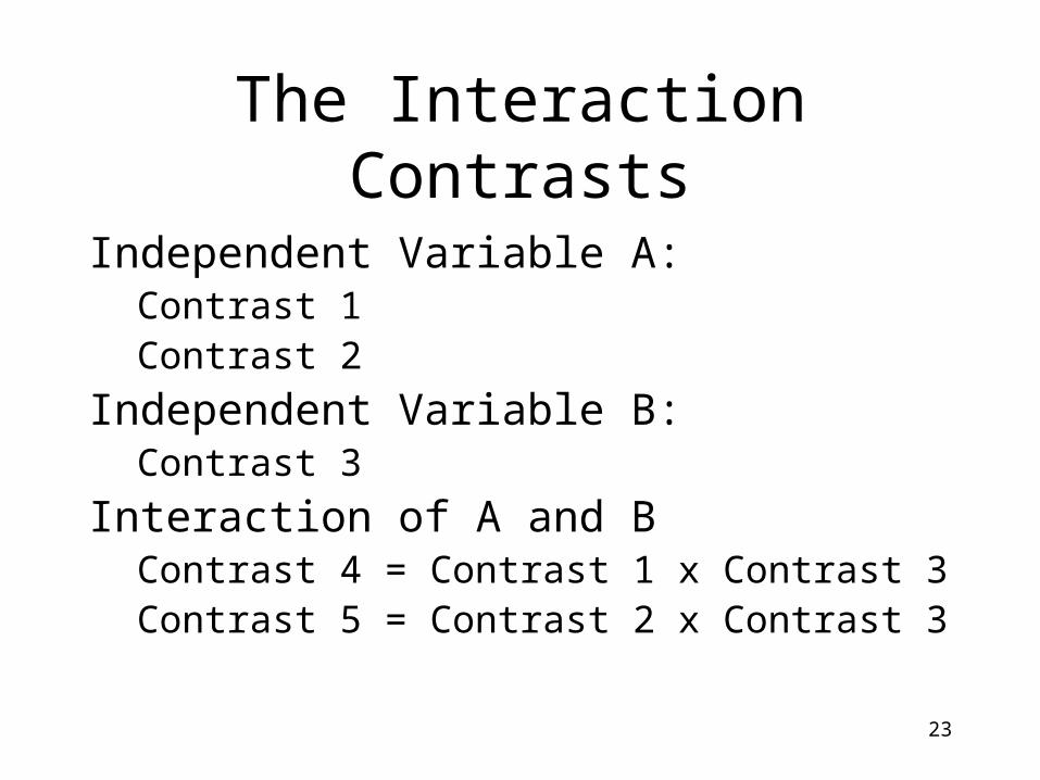
Independent Variable A:Contrast 1Contrast 2

Independent Variable B:Contrast 3

Interaction of A and BContrast 4 = Contrast 1 x Contrast 3Contrast 5 = Contrast 2 x Contrast 3

24

Interaction Contrasts

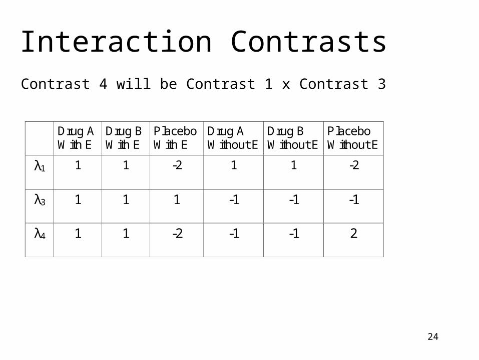
Contrast 4 will be Contrast 1 x Contrast 3

Drug A With E

Drug B With E

Placebo With E

Drug A Without E

Drug B Without E

Placebo Without E

λ1 1 1 -2 1 1 -2

λ3 1 1 1 -1 -1 -1

λ4 1 1 -2 -1 -1 2

25

What Does Contrast 4 test?

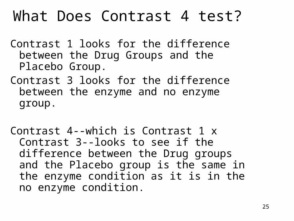
Contrast 1 looks for the difference between the Drug Groups and the Placebo Group.

Contrast 3 looks for the difference between the enzyme and no enzyme group.

Contrast 4--which is Contrast 1 x Contrast 3--looks to see if the difference between the Drug groups and the Placebo group is the same in the enzyme condition as it is in the no enzyme condition.

26

02

---or- 2

:0 PlaceboDrug_BDrug_A

PlaceboDrug_BDrug_A

H

:0 zymeWithout_EneWith_Enzym H

Condition) Enzyme Without (in the Condition) Enzyme With (in the

PlaceboDrug_BDrug_A

PlaceboDrug_BDrug_A

2

2:0

H

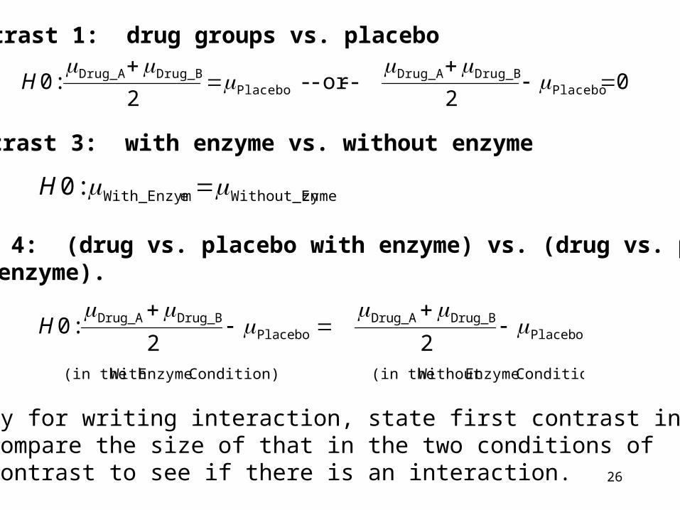
Contrast 1: drug groups vs. placebo

Contrast 3: with enzyme vs. without enzyme

Contrast 4: (drug vs. placebo with enzyme) vs. (drug vs. placebowithout enzyme).

Note strategy for writing interaction, state first contrast in its ‘=0’form, then compare the size of that in the two conditions ofthe second contrast to see if there is an interaction.

27

Interaction Contrasts

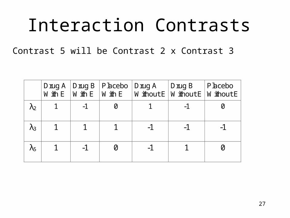
Contrast 5 will be Contrast 2 x Contrast 3

Drug A With E

Drug B With E

Placebo With E

Drug A Without E

Drug B Without E

Placebo Without E

λ2 1 -1 0 1 -1 0

λ3 1 1 1 -1 -1 -1

λ5 1 -1 0 -1 1 0

28

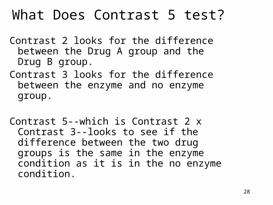
What Does Contrast 5 test?

Contrast 2 looks for the difference between the Drug A group and the Drug B group.

Contrast 3 looks for the difference between the enzyme and no enzyme group.

Contrast 5--which is Contrast 2 x Contrast 3--looks to see if the difference between the two drug groups is the same in the enzyme condition as it is in the no enzyme condition.

29

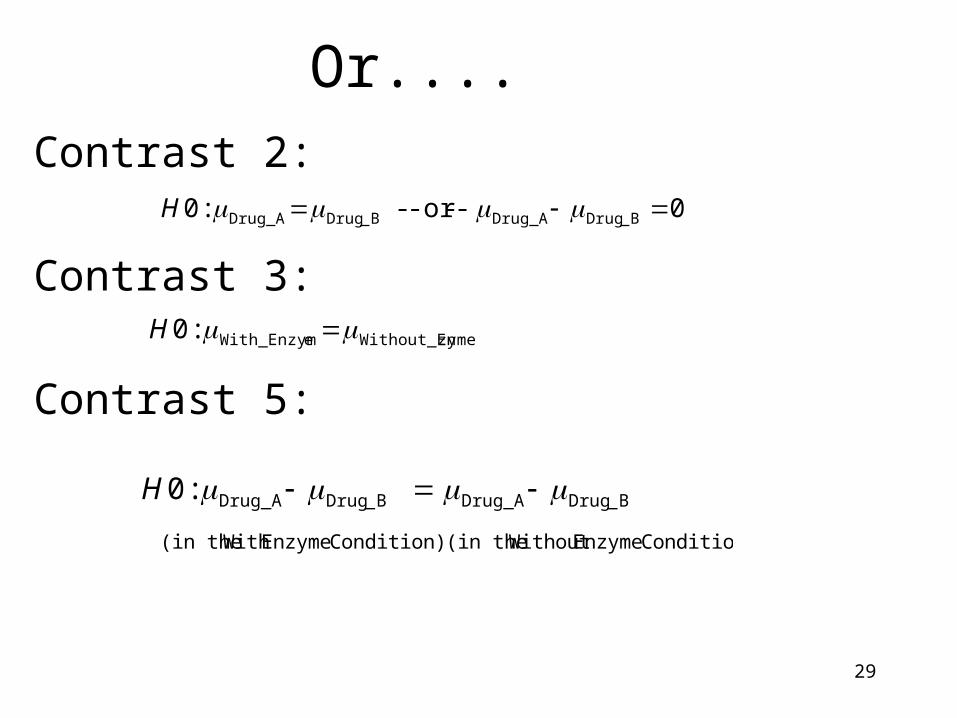
Or....Contrast 2:

Contrast 3:

Contrast 5:

0 ---or- :0 B_DrugDrug_AB_DrugDrug_A H

:0 zymeWithout_EneWith_Enzym H

Condition) Enzyme Without (in the Condition) Enzyme With (in the

B_DrugDrug_AB_DrugDrug_A :0 H

30

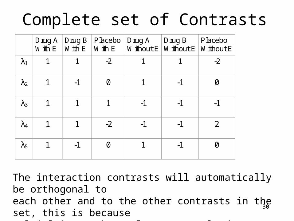
Complete set of Contrasts Drug A

With E Drug B With E

Placebo With E

Drug A Without E

Drug B Without E

Placebo Without E

λ1 1 1 -2 1 1 -2

λ2 1 -1 0 1 -1 0

λ3 1 1 1 -1 -1 -1

λ4 1 1 -2 -1 -1 2

λ5 1 -1 0 1 -1 0

The interaction contrasts will automatically be orthogonal toeach other and to the other contrasts in the set, this is becausemultiplying orthogonal contrasts leads to an orthogonal contrast.

31

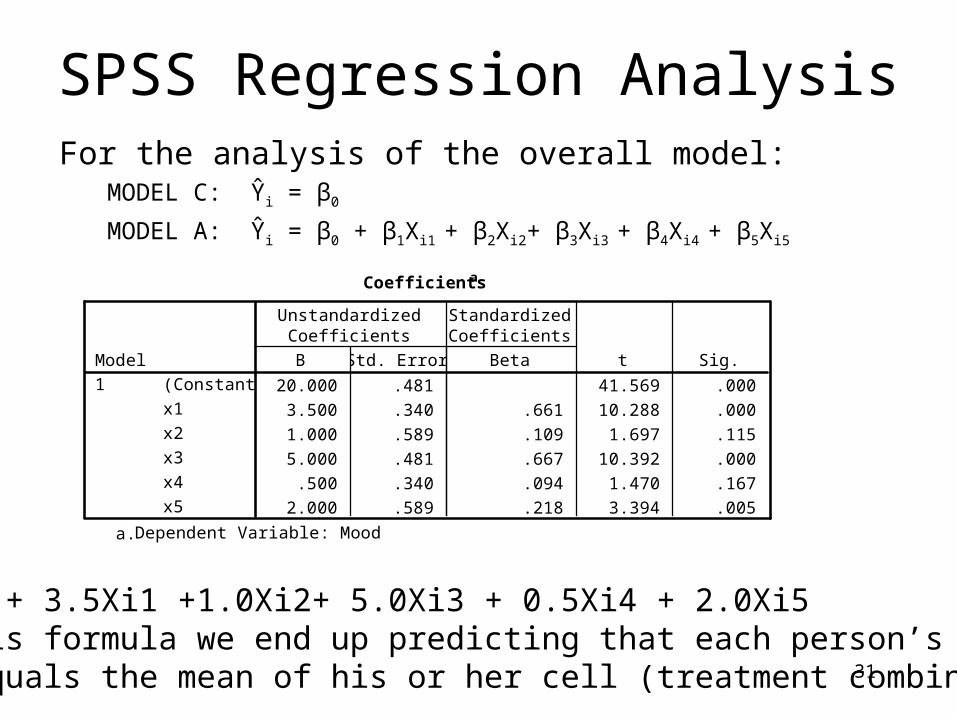
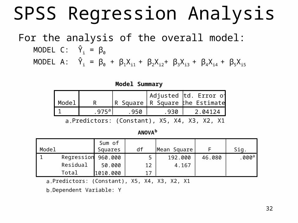
SPSS Regression AnalysisFor the analysis of the overall model:

MODEL C: Ŷi = β0

MODEL A: Ŷi = β0 + β1Xi1 + β2Xi2+ β3Xi3 + β4Xi4 + β5Xi5

Coefficientsa

20.000 .481 41.569 .000

3.500 .340 .661 10.288 .000

1.000 .589 .109 1.697 .115

5.000 .481 .667 10.392 .000

.500 .340 .094 1.470 .167

2.000 .589 .218 3.394 .005

(Constant)

x1

x2

x3

x4

x5

Model1

B Std. Error

UnstandardizedCoefficients

Beta

StandardizedCoefficients

t Sig.

Dependent Variable: Mooda.

Ŷi = 20 + 3.5Xi1 +1.0Xi2+ 5.0Xi3 + 0.5Xi4 + 2.0Xi5With this formula we end up predicting that each person’sscore equals the mean of his or her cell (treatment combination)

32

SPSS Regression Analysis

Model Summary

.975a .950 .930 2.04124Model1

R R SquareAdjustedR Square

Std. Error ofthe Estimate

Predictors: (Constant), X5, X4, X3, X2, X1a.

ANOVAb

960.000 5 192.000 46.080 .000a

50.000 12 4.167

1010.000 17

Regression

Residual

Total

Model1

Sum ofSquares df Mean Square F Sig.

Predictors: (Constant), X5, X4, X3, X2, X1a.

Dependent Variable: Yb.

For the analysis of the overall model:MODEL C: Ŷi = β0

MODEL A: Ŷi = β0 + β1Xi1 + β2Xi2+ β3Xi3 + β4Xi4 + β5Xi5

33

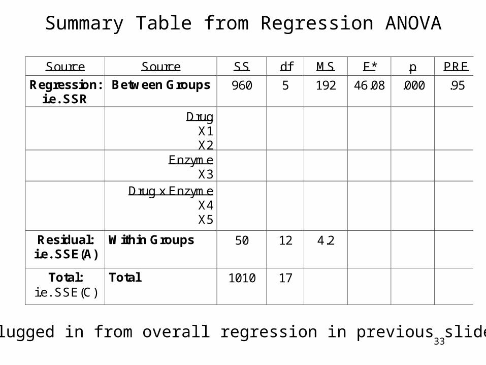
Summary Table from Regression ANOVA

Source Source SS df MS F* p PRE

Regression: i.e. SSR

Between Groups 960 5

192 46.08 .000 .95

Drug X1 X2

Enzyme X3

Drug x Enzyme X4 X5

Residual: i.e. SSE(A)

Within Groups 50 12

4.2

Total: i.e. SSE(C)

Total 1010 17

Values plugged in from overall regression in previous slide.

34

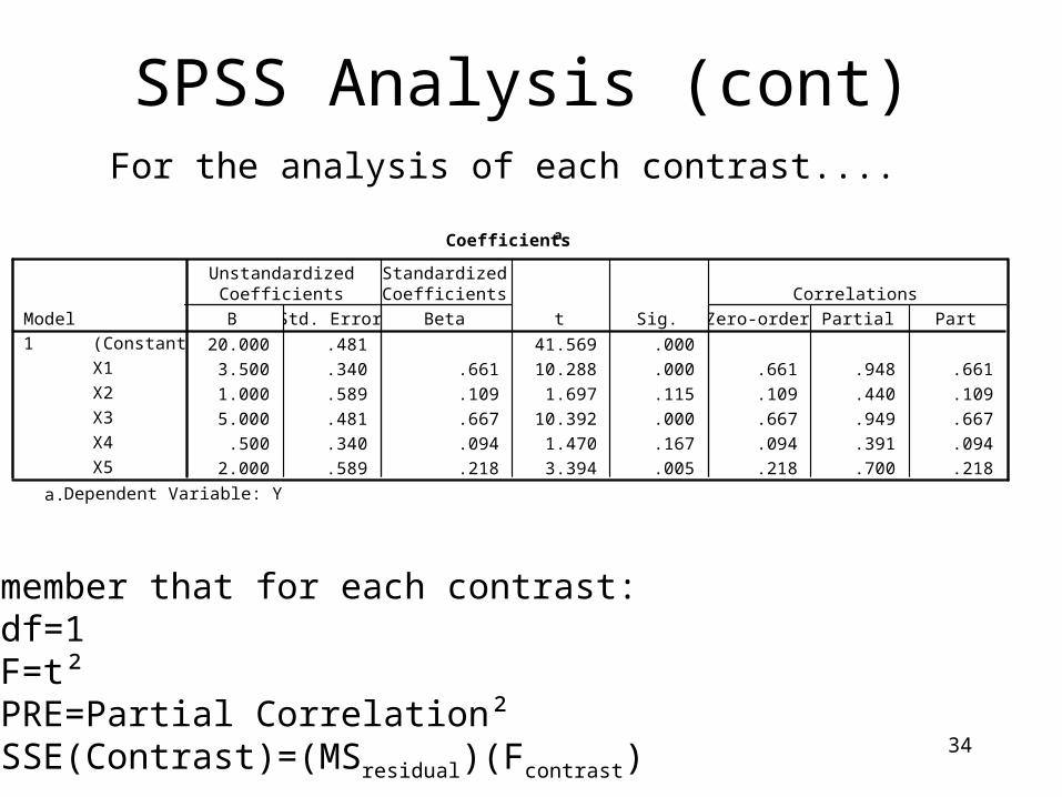
SPSS Analysis (cont)

Coefficientsa

20.000 .481 41.569 .000

3.500 .340 .661 10.288 .000 .661 .948 .661

1.000 .589 .109 1.697 .115 .109 .440 .109

5.000 .481 .667 10.392 .000 .667 .949 .667

.500 .340 .094 1.470 .167 .094 .391 .094

2.000 .589 .218 3.394 .005 .218 .700 .218

(Constant)

X1

X2

X3

X4

X5

Model1

B Std. Error

UnstandardizedCoefficients

Beta

StandardizedCoefficients

t Sig. Zero-order Partial Part

Correlations

Dependent Variable: Ya.

Remember that for each contrast: df=1 F=t² PRE=Partial Correlation² SSE(Contrast)=(MSresidual)(Fcontrast)

For the analysis of each contrast....

35

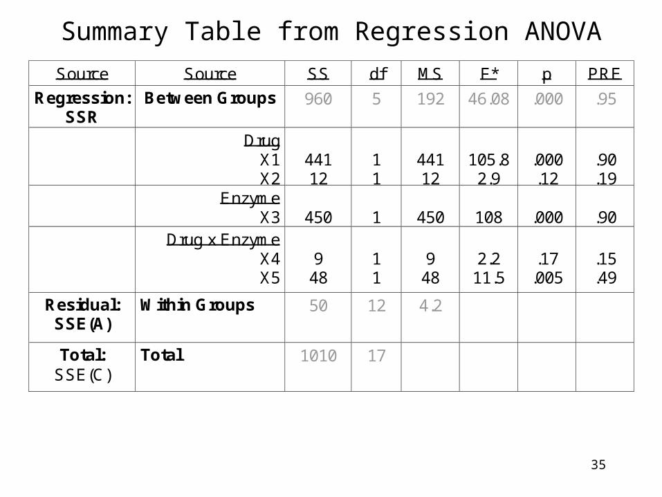
Summary Table from Regression ANOVA

Source Source SS df MS F* p PRE

Regression: SSR

Between Groups 960 5

192 46.08 .000 .95

Drug X1 X2

441 12

1 1

441 12

105.8

2.9

.000 .12

.90 .19

Enzyme X3

450

1

450

108

.000

.90

Drug x Enzyme X4 X5

9

48

1 1

9

48

2.2

11.5

.17

.005

.15 .49

Residual: SSE(A)

Within Groups 50 12

4.2

Total: SSE(C)

Total 1010 17

36

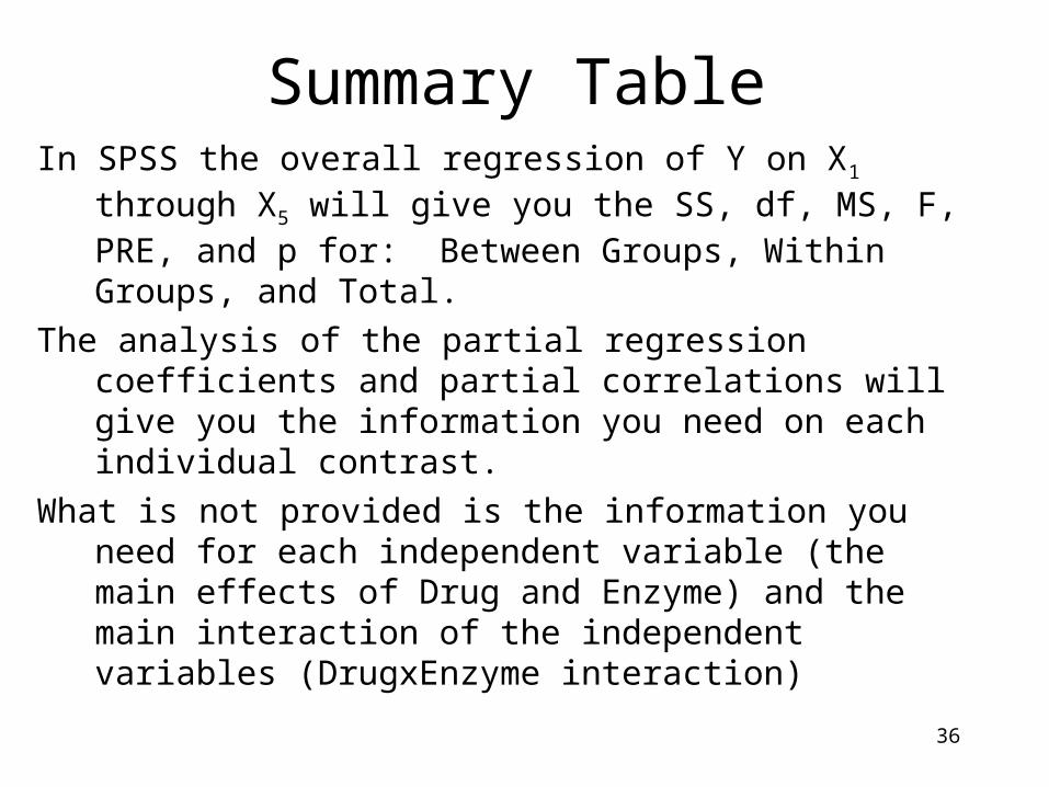
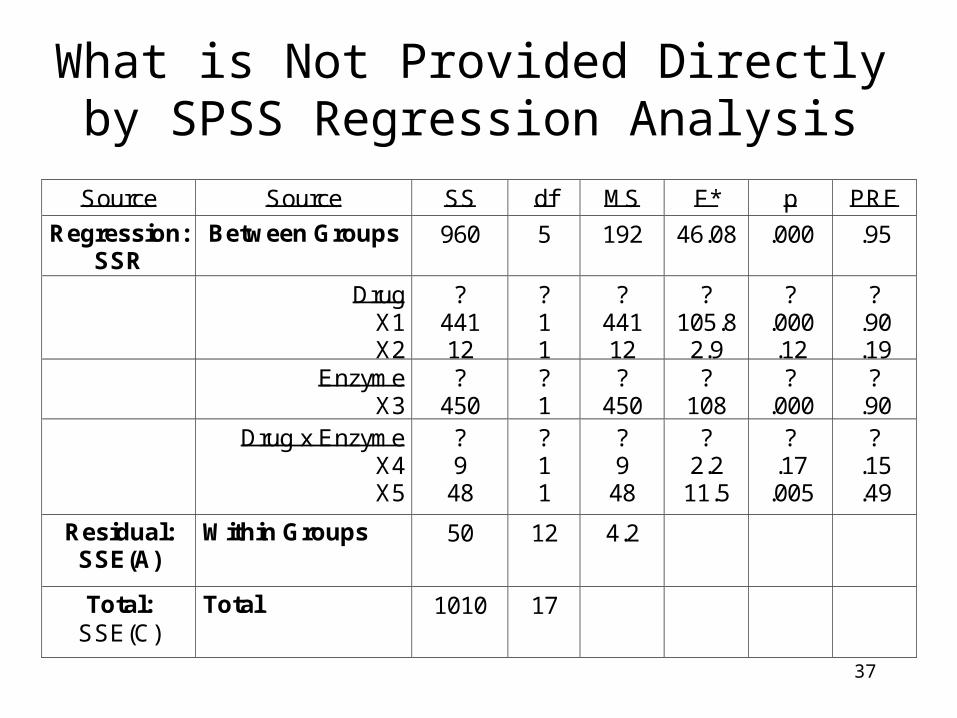
Summary TableIn SPSS the overall regression of Y on X1 through X5

will give you the SS, df, MS, F, PRE, and p for: Between Groups, Within Groups, and Total.

The analysis of the partial regression coefficients and partial correlations will give you the information you need on each individual contrast.

What is not provided is the information you need for each independent variable (the main effects of Drug and Enzyme) and the main interaction of the independent variables (DrugxEnzyme interaction)

37

What is Not Provided Directly by SPSS Regression Analysis

Source Source SS df MS F* p PRE

Regression: SSR

Between Groups 960 5

192 46.08 .000 .95

Drug X1 X2

? 441 12

? 1 1

? 441 12

? 105.8

2.9

? .000 .12

? .90 .19

Enzyme X3

? 450

? 1

? 450

? 108

? .000

? .90

Drug x Enzyme X4 X5

? 9

48

? 1 1

? 9

48

? 2.2

11.5

? .17

.005

? .15 .49

Residual: SSE(A)

Within Groups 50 12

4.2

Total: SSE(C)

Total 1010 17

38

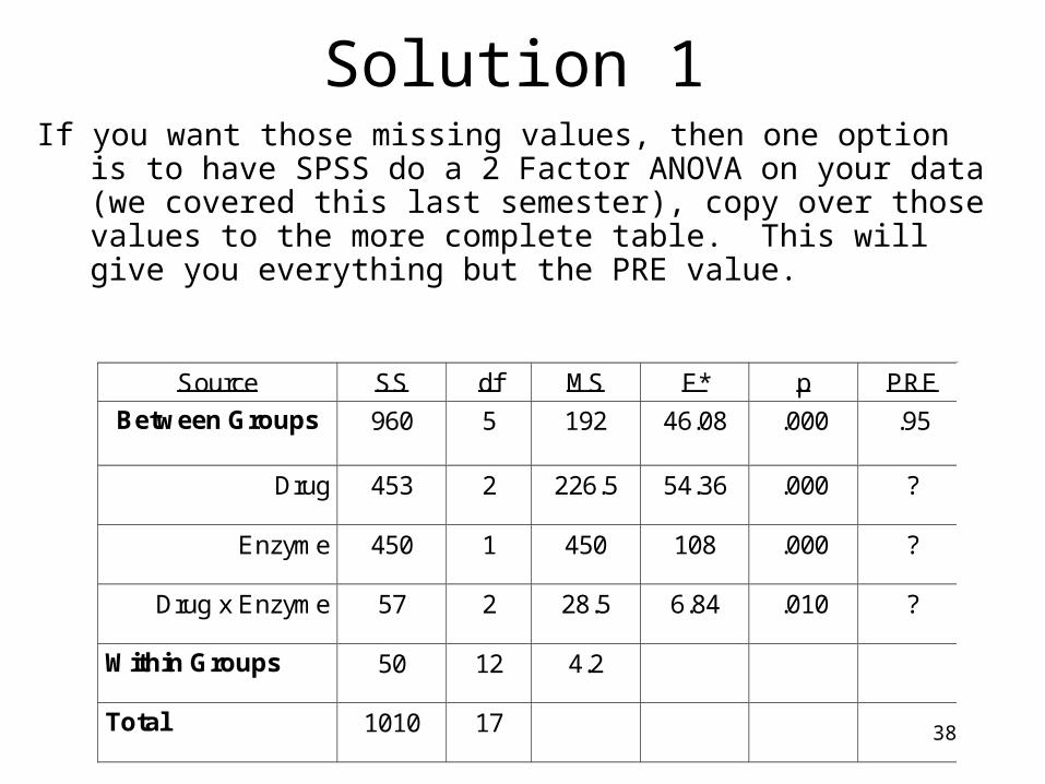
Solution 1If you want those missing values, then one option is to have

SPSS do a 2 Factor ANOVA on your data (we covered this last semester), copy over those values to the more complete table. This will give you everything but the PRE value.

Source SS df MS F* p PRE

Between Groups 960 5

192 46.08 .000 .95

Drug

453

2

226.5

54.36

.000

?

Enzyme

450

1

450

108

.000

?

Drug x Enzyme

57

2

28.5

6.84

.010

?

Within Groups 50 12

4.2

Total 1010 17

39

Solution 1 (cont.)

PRE = (SS for the variable) / (SS for the variable + SS Within Groups)

40

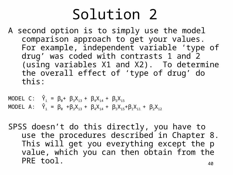
Solution 2A second option is to simply use the model comparison

approach to get your values. For example, independent variable ‘type of drug’ was coded with contrasts 1 and 2 (using variables X1 and X2). To determine the overall effect of ‘type of drug’ do this:

MODEL C: Ŷi = β0+ β3Xi3 + β4Xi4 + β5Xi5

MODEL A: Ŷi = β0 +β3Xi3 + β4Xi4 + β5Xi5+β1Xi1 + β2Xi2

SPSS doesn’t do this directly, you have to use the procedures described in Chapter 8. This will get you everything except the p value, which you can then obtain from the PRE tool.

41

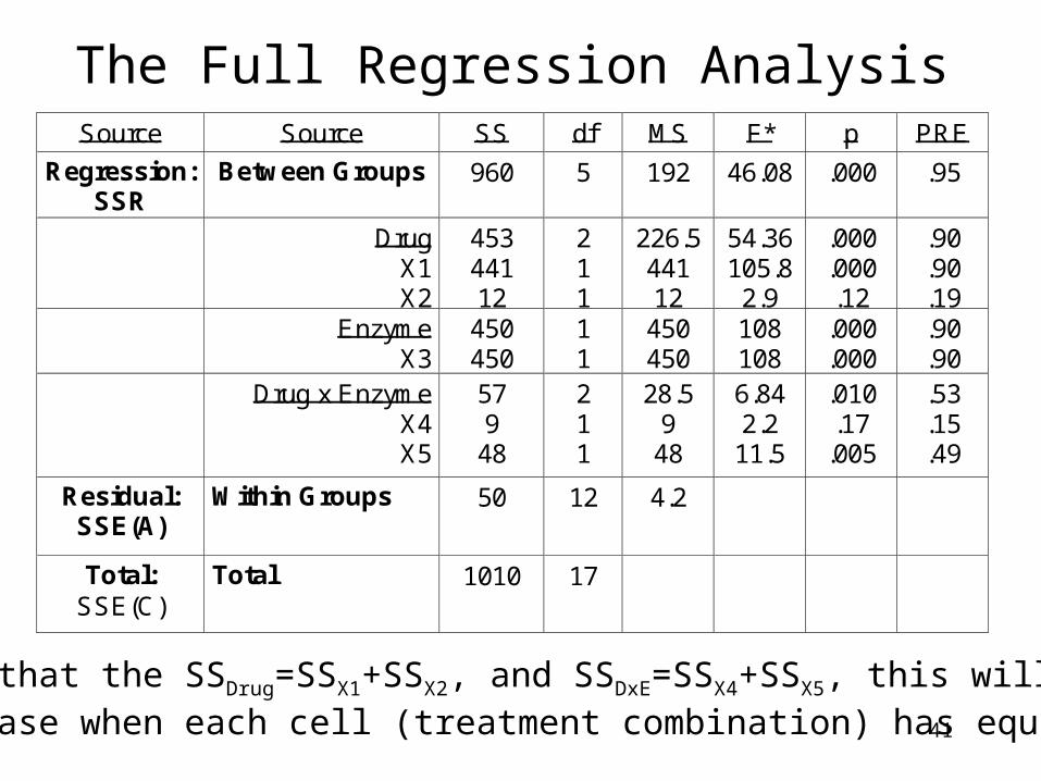
The Full Regression AnalysisSource Source SS df MS F* p PRE

Regression: SSR

Between Groups 960 5

192 46.08 .000 .95

Drug X1 X2

453 441 12

2 1 1

226.5 441 12

54.36 105.8

2.9

.000

.000 .12

.90

.90

.19 Enzyme

X3 450 450

1 1

450 450

108 108

.000

.000 .90 .90

Drug x Enzyme X4 X5

57 9

48

2 1 1

28.5 9

48

6.84 2.2

11.5

.010 .17

.005

.53

.15

.49

Residual: SSE(A)

Within Groups 50 12

4.2

Total: SSE(C)

Total 1010 17

Note that the SSDrug=SSX1+SSX2, and SSDxE=SSX4+SSX5, this will bethe case when each cell (treatment combination) has equal N.

42

Source Source SS df MS F* p PRE

Regression: SSR

Between Groups 960 5

192 46.08 .000 .95

Drug X1 X2

453 441 12

2 1 1

226.5 441 12

54.36 105.8

2.9

.000

.000 .12

.90

.90

.19 Enzyme

X3 450 450

1 1

450 450

108 108

.000

.000 .90 .90

Drug x Enzyme X4 X5

57 9

48

2 1 1

28.5 9

48

6.84 2.2

11.5

.010 .17

.005

.53

.15

.49

Residual: SSE(A)

Within Groups 50 12

4.2

Total: SSE(C)

Total 1010 17

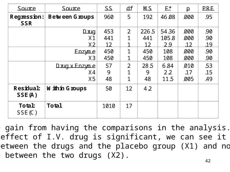
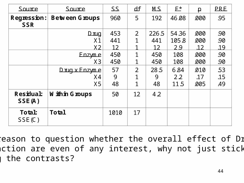
Note what we gain from having the comparisons in the analysis. Whilethe overall effect of I.V. drug is significant, we can see it is due to thedifference between the drugs and the placebo group (X1) and not due toa difference between the two drugs (X2).

43

Source Source SS df MS F* p PRE

Regression: SSR

Between Groups 960 5

192 46.08 .000 .95

Drug X1 X2

453 441 12

2 1 1

226.5 441 12

54.36 105.8

2.9

.000

.000 .12

.90

.90

.19 Enzyme

X3 450 450

1 1

450 450

108 108

.000

.000 .90 .90

Drug x Enzyme X4 X5

57 9

48

2 1 1

28.5 9

48

6.84 2.2

11.5

.010 .17

.005

.53

.15

.49

Residual: SSE(A)

Within Groups 50 12

4.2

Total: SSE(C)

Total 1010 17

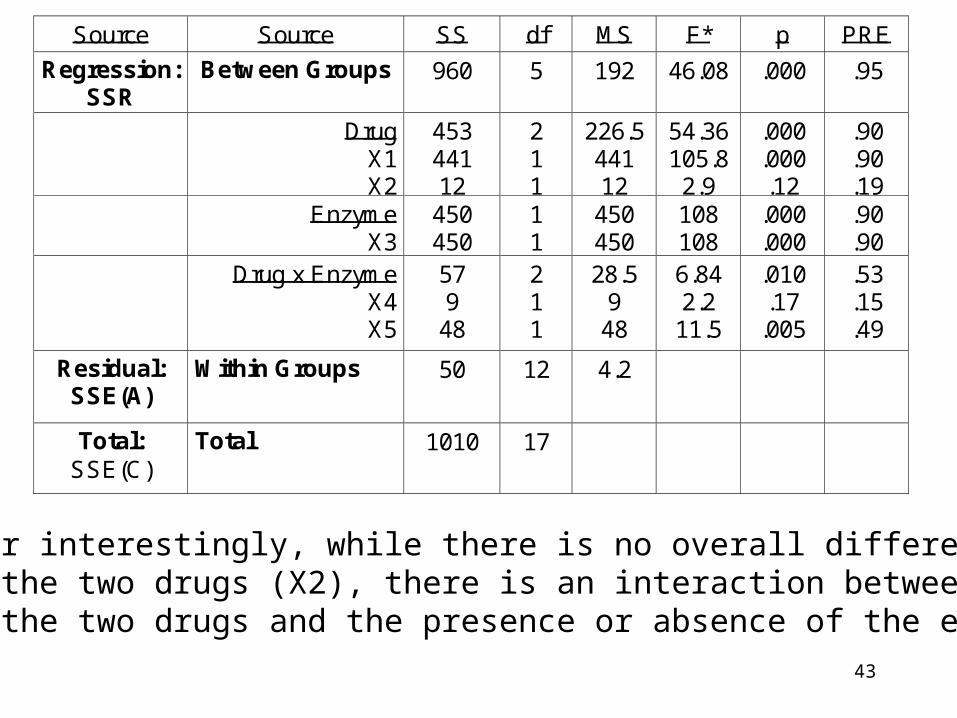
And, rather interestingly, while there is no overall difference in theeffect of the two drugs (X2), there is an interaction between theeffect of the two drugs and the presence or absence of the enzyme (X5).

44

Source Source SS df MS F* p PRE

Regression: SSR

Between Groups 960 5

192 46.08 .000 .95

Drug X1 X2

453 441 12

2 1 1

226.5 441 12

54.36 105.8

2.9

.000

.000 .12

.90

.90

.19 Enzyme

X3 450 450

1 1

450 450

108 108

.000

.000 .90 .90

Drug x Enzyme X4 X5

57 9

48

2 1 1

28.5 9

48

6.84 2.2

11.5

.010 .17

.005

.53

.15

.49

Residual: SSE(A)

Within Groups 50 12

4.2

Total: SSE(C)

Total 1010 17

There is reason to question whether the overall effect of Drug, Enzymeand Interaction are even of any interest, why not just stick with evaluating the contrasts?

45

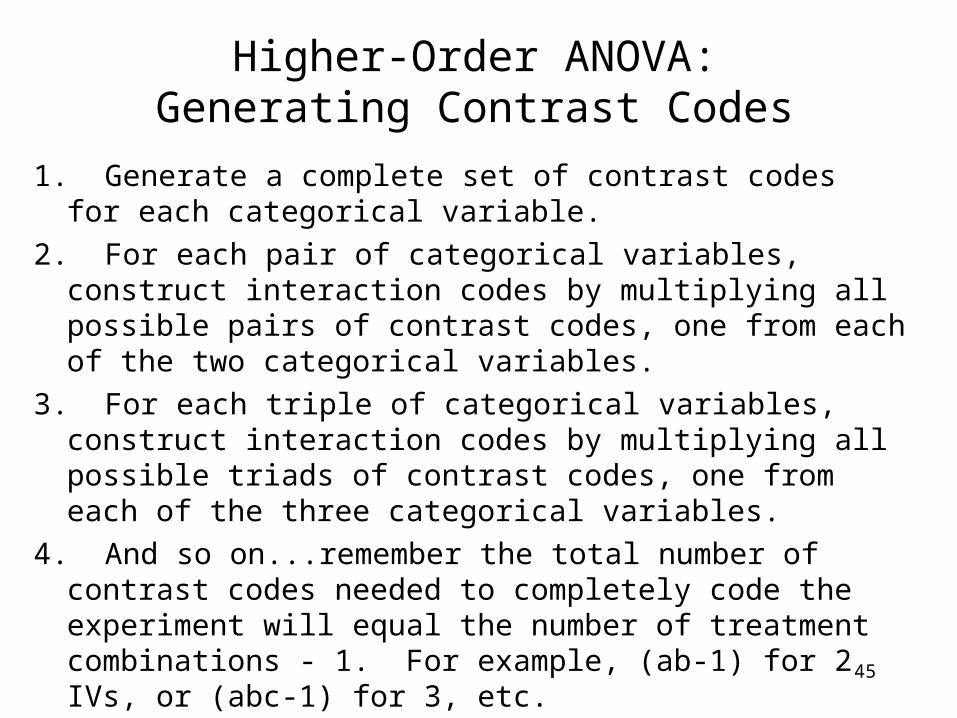
Higher-Order ANOVA:Generating Contrast Codes

1. Generate a complete set of contrast codes for each categorical variable.

2. For each pair of categorical variables, construct interaction codes by multiplying all possible pairs of contrast codes, one from each of the two categorical variables.

3. For each triple of categorical variables, construct interaction codes by multiplying all possible triads of contrast codes, one from each of the three categorical variables.

4. And so on...remember the total number of contrast codes needed to completely code the experiment will equal the number of treatment combinations - 1. For example, (ab-1) for 2 IVs, or (abc-1) for 3, etc.

46

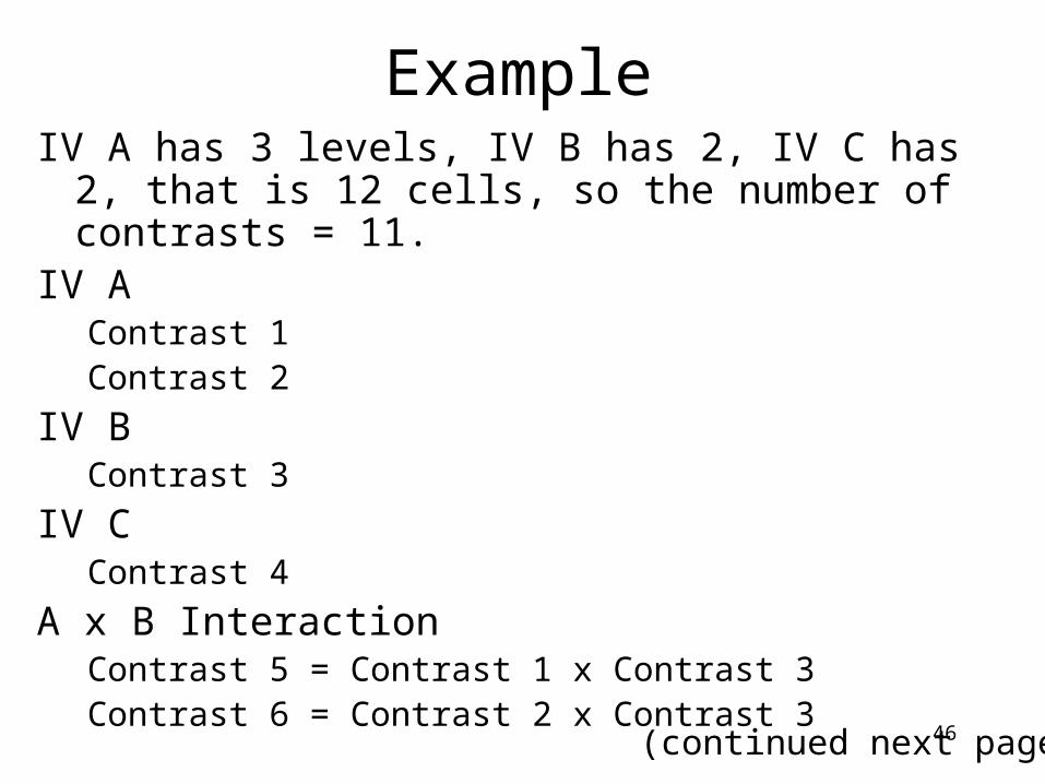
ExampleIV A has 3 levels, IV B has 2, IV C has 2, that is 12 cells,

so the number of contrasts = 11.IV A

Contrast 1Contrast 2

IV BContrast 3

IV CContrast 4

A x B InteractionContrast 5 = Contrast 1 x Contrast 3Contrast 6 = Contrast 2 x Contrast 3

(continued next page)

47

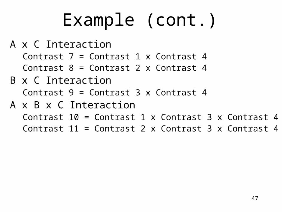
Example (cont.)A x C Interaction

Contrast 7 = Contrast 1 x Contrast 4Contrast 8 = Contrast 2 x Contrast 4

B x C InteractionContrast 9 = Contrast 3 x Contrast 4

A x B x C InteractionContrast 10 = Contrast 1 x Contrast 3 x Contrast 4Contrast 11 = Contrast 2 x Contrast 3 x Contrast 4

48

Yikes!The process of generating contrast codes can lead

to a large number of codes in a factorial design, the 4x3x2 design in the example in the book leads to 23 contrasts (4x3x2-1), 6 of which involve triple interactions. These are rarely all of a priori interest, let alone understandable.

49

Galloping (Type 1) Error Rates

Remember from last semester, if we make many null hypothesis significance tests, and if H0 is true for all of them, then the probability of making at least one Type 1 error (rejecting H0 when H0 is false) becomes unacceptably high. Also, remember that the probability of making a type 1 error when H0 is true in any particular test equals our significance level, usually .05.

50

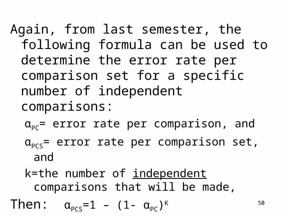
Again, from last semester, the following formula can be used to determine the error rate per comparison set for a specific number of independent comparisons: αPC= error rate per comparison, and

αPCS= error rate per comparison set, and

k=the number of independent comparisons that will be made,

Then: αPCS=1 – (1- αPC)K

With 23 contrasts αPCS=1 – (1- .05)23 =0.70

51

All 23 contrasts are independent of each other as they are orthogonal, if each comparison has a .05 chance of making a type 1 error then the error rate for the whole analysis equals .70.

There is a good chance that some of these comparison will be significant just due to chance, and that in turn could cause you to spend a great deal of time and energy tying your theory (and your brain) into knots trying to explain them.

52

SolutionProbably the best solution is to attend carefully to which

of these contrasts have a priori interest, either because they replicate previous studies or because they test specific theories you are investigating. Before you gather your data make a list of which contrasts have a priori interest and make those the focus of your analysis. For those you can either simply use either .05 or (.05)/(# of a priori contrasts) as your significance level (I would choose the latter if there were more than just a few a priori comparisons), then use Scheffe’s for the other (a posteriori) comparisons. In determining how to handle error rate remember, you are trying to understand your data, not get brownie points for the number of significant results.

53

Solution (cont.)

Any contrasts that look interesting a posteriori might play a role in what study you do next. There might be something really interesting that crops up, but be aware that it might well just be just due to chance, you might not want to invest a lot of thought and energy into pursuing it until you find if it can be replicated.

You could also choose to just note any interesting contrasts and then see if they appear again in later studies before you investigate further.

54

Three Thoughts (1)

While it may be a bother to work out all of the contrasts to do the equivalent of a factorial ANOVA, remember that you gain several things by doing so:

1. Deciding upon the comparisons helps insure that you are thinking quite specifically about your theory and what you are trying to test in the analysis.

55

Three Thoughts (2)

2. Comparisons give you much more specific information about what is going on among the groups, going beyond simply asking did anything happen? This seems particularly true to me as we work our way up into the interactions. Go back to our example with the complete summary table to see what we gained in understanding by having the contrasts in our analysis.

56

Three Thoughts (3)

3. Comparisons have more power than the overall (main) effects. If an independent variable is coded with three contrasts, then the test for the overall effect of that independent variable is based upon the PRE per parameter added (in this case three parameters, one for each contrast). If one of those contrasts is strong and the other two weak, then the PRE per parameter added for the independent variable considered as a whole may not be statistically significant.

57

More on Power

So, if an independent variable is coded with more than one contrast, the tests for the statistical significance of each contrast will be more powerful than the test for the overall effect of the independent variable.

There is, in addition, another statement to be made about power, and that is that the power of the test for any part of the analysis (individual contrasts or the overall effect of an independent variable) is likely to be greater in a factorial design than in a design that looks at each contrast, or each independent variable, separately. The following slides will (I hope) make this clear.

58

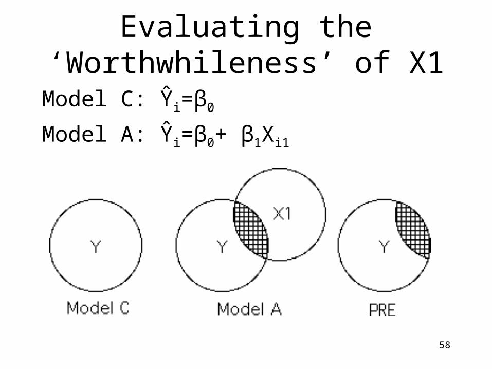
Evaluating the ‘Worthwhileness’ of X1

Model C: Ŷi=β0

Model A: Ŷi=β0+ β1Xi1

59

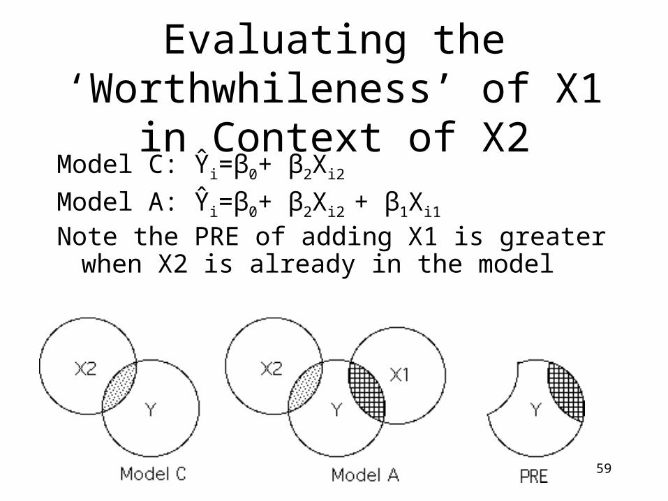
Evaluating the ‘Worthwhileness’ of X1 in Context of X2

Model C: Ŷi=β0+ β2Xi2

Model A: Ŷi=β0+ β2Xi2 + β1Xi1

Note the PRE of adding X1 is greater when X2 is already in the model

60

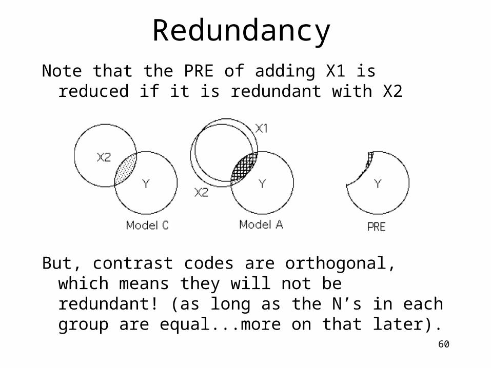
RedundancyNote that the PRE of adding X1 is reduced if it is

redundant with X2

But, contrast codes are orthogonal, which means they will not be redundant! (as long as the N’s in each group are equal...more on that later).

61

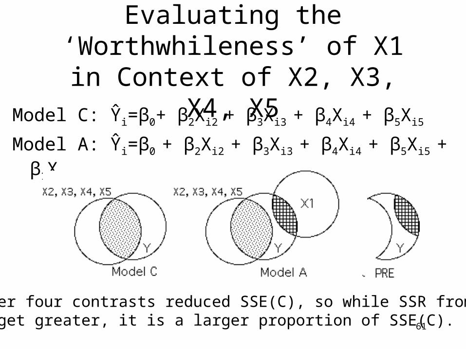
Evaluating the ‘Worthwhileness’ of X1 in Context of X2, X3, X4, X5

Model C: Ŷi=β0+ β2Xi2 + β3Xi3 + β4Xi4 + β5Xi5

Model A: Ŷi=β0 + β2Xi2 + β3Xi3 + β4Xi4 + β5Xi5 + β1Xi1

The other four contrasts reduced SSE(C), so while SSR from X1didn’t get greater, it is a larger proportion of SSE(C).

62

Unequal N’s

As in the previous chapter, there is no particular reason why the n’s in each treatment cell have to be equal, if they are not then:

1. SS for an independent variable will probably not equal the sum of the SS for its contrasts.

2. There could be a loss of power due to redundancies that appear between the contrasts due to the unequal n’s. It is important to look at the tolerances of the contrasts so that you can appropriate interpret a lack of significance (i.e. it could be due to low tolerance rather than to low effect).

63

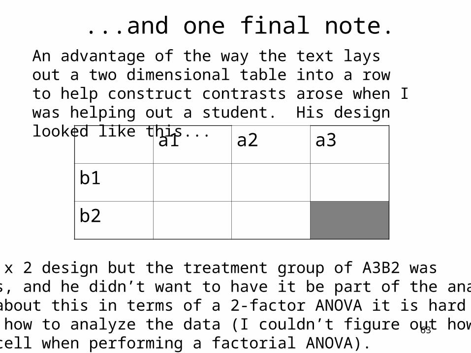
...and one final note.An advantage of the way the text lays out a two dimensional table into a row to help construct contrasts arose when I was helping out a student. His design looked like this...

a1 a2 a3

b1

b2

It was a 3 x 2 design but the treatment group of A3B2 was meaningless, and he didn’t want to have it be part of the analysis. Ifyou think about this in terms of a 2-factor ANOVA it is hard to figure out how to analyze the data (I couldn’t figure out how toexclude a cell when performing a factorial ANOVA).

64

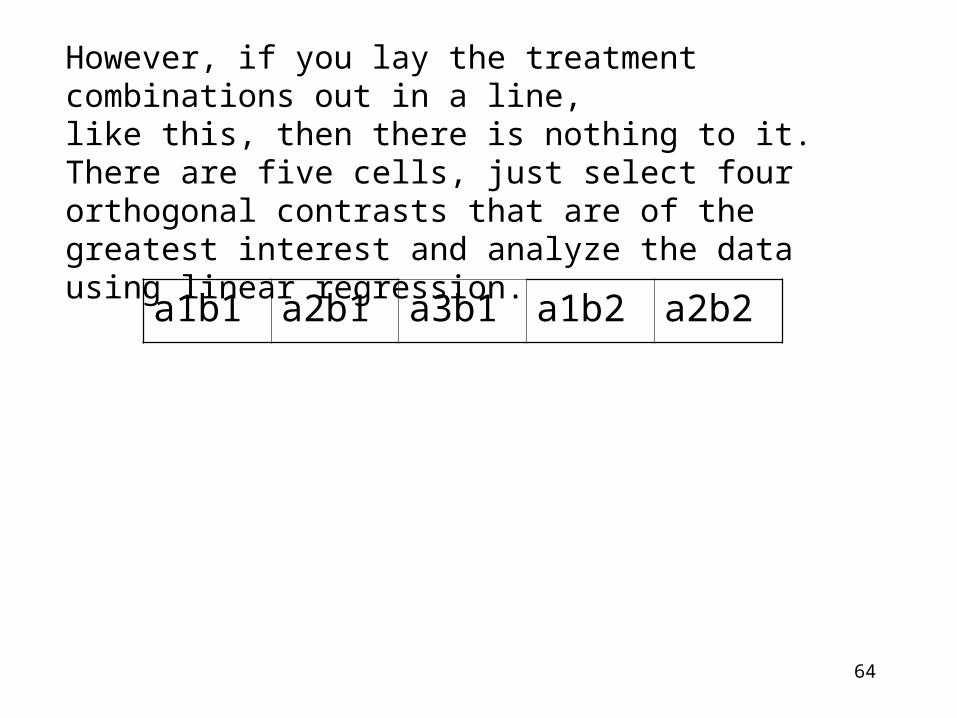
However, if you lay the treatment combinations out in a line,like this, then there is nothing to it. There are five cells, just select four orthogonal contrasts that are of the greatest interest and analyze the data using linear regression.

a1b1 a2b1 a3b1 a1b2 a2b2