1

Predicting peaks and troughs in real house prices: a probit

approach

LIME WorkshopBrussels, 8 December 2011

Paul van den Noord

2

Sharp reboundsReal house prices, index 2009Q1 = 100

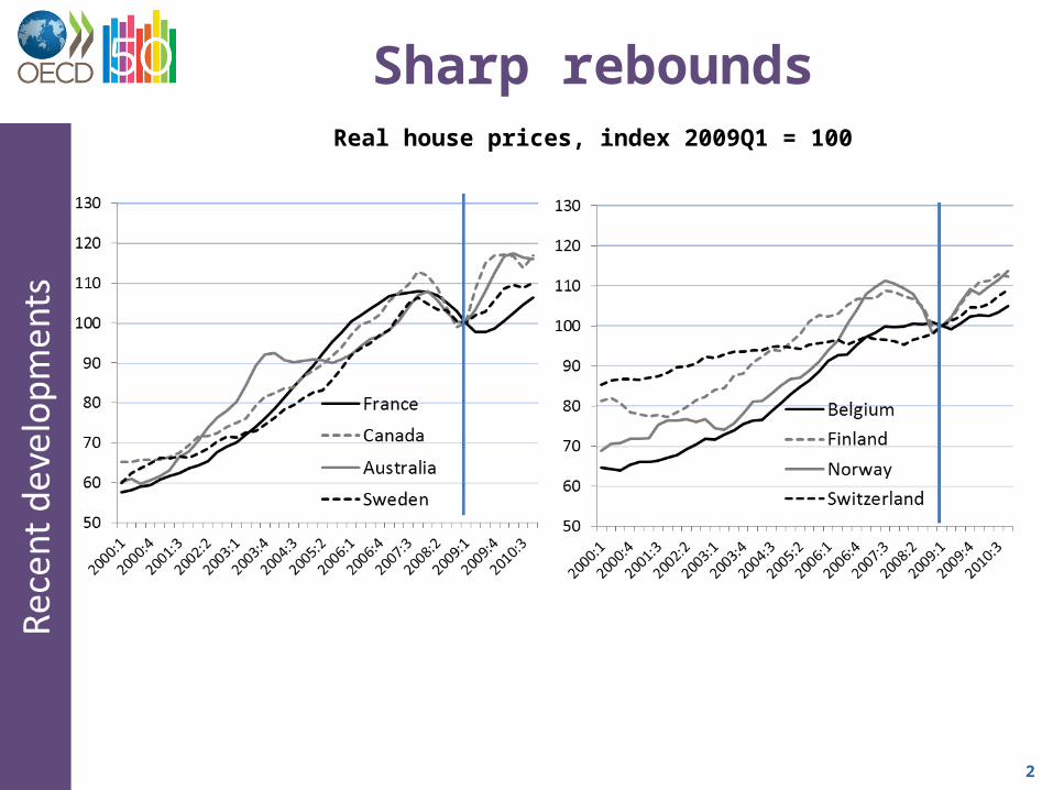
3

Weak or faltering reboundsReal house prices, index 2009Q1 = 100

4

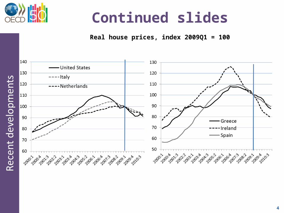
Continued slidesReal house prices, index 2009Q1 = 100

5

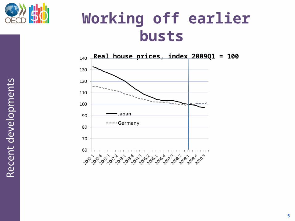
Working off earlier busts Real house prices, index 2009Q1 = 100

6

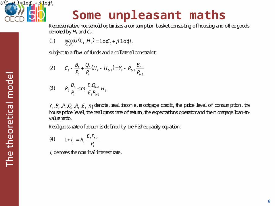
Some unpleasant mathsRepresentative household optimises a consumption basket consisting of housing and other goods, denoted by Ht and Ct:

(1) ttHC

HCUtt

,max, tt HC loglog

subject to a flow of funds and a collateral constraint:

(2) 1

111

t

ttttt

t

t

t

tt P

BRYHH

P

Q

P

BC

(3) t

tt

ttt

t

tt H

PE

QEm

P

BR

1

1

ttttttt mERQPBY ,,,,,, denote, real income, mortgage credit, the price level of consumption, the

house price level, the real gross rate of return, the expectations operator and the mortgage loan-to-value ratio.

Real gross rate of return is defined by the Fisher parity equation:

(4) t

tttt

P

PERi 11

it denotes the nominal interest rate.

tttt HCHCU loglog,

7

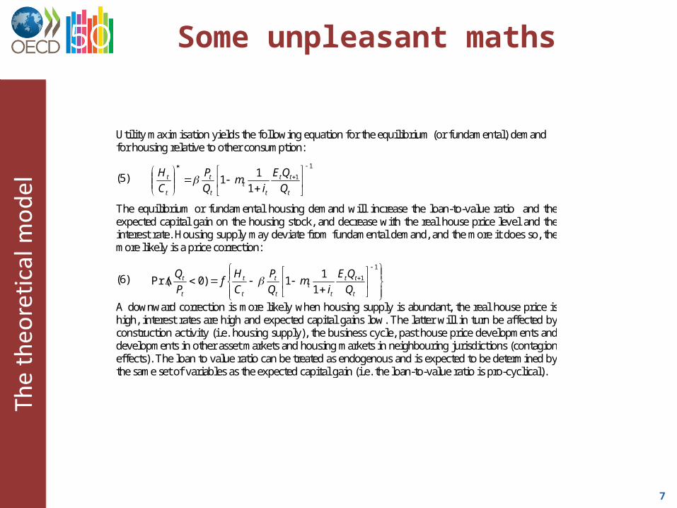
Some unpleasant maths

Utility maximisation yields the following equation for the equilibrium (or fundamental) demand for housing relative to other consumption:

(5) 1

1

1

11

t

tt

tt

t

t

t

t

Q

QE

im

Q

P

C

H

The equilibrium or fundamental housing demand will increase the loan-to-value ratio and the expected capital gain on the housing stock, and decrease with the real house price level and the interest rate. Housing supply may deviate from fundamental demand, and the more it does so, the more likely is a price correction:

(6)

1

1

1

11)0Pr(

t

tt

tt

t

t

t

t

t

t

Q

QE

im

Q

P

C

Hf

P

Q

A downward correction is more likely when housing supply is abundant, the real house price is high, interest rates are high and expected capital gains low. The latter will in turn be affected by construction activity (i.e. housing supply), the business cycle, past house price developments and developments in other asset markets and housing markets in neighbouring jurisdictions (contagion effects). The loan to value ratio can be treated as endogenous and is expected to be determined by the same set of variables as the expected capital gain (i.e. the loan-to-value ratio is pro-cyclical).

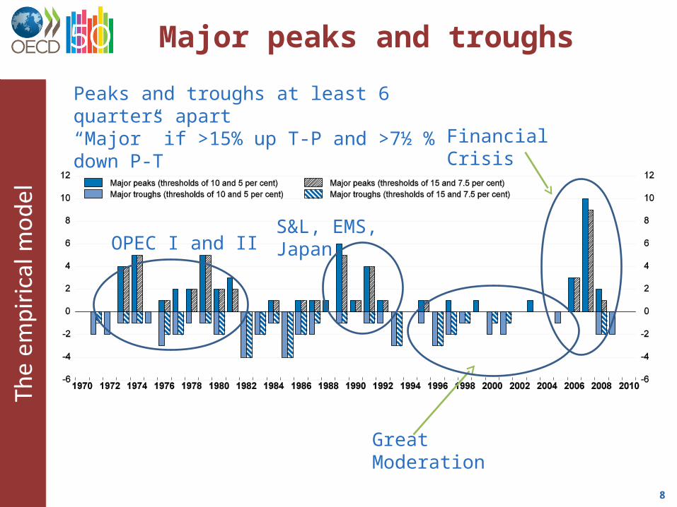
8

Major peaks and troughs

Great Moderation

Financial Crisis

S&L, EMS, Japan OPEC I and II

Peaks and troughs at least 6 quarters apart“Major” if >15% up T-P and >7½ % down P-T

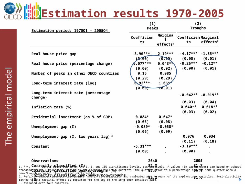
9

Estimation results 1970-2005

(1)Peaks

(2)Troughs

Estimation period: 1970Q1 – 2005Q4

CoefficientsMarginal effects2

CoefficientsMarginal effects2

Real house price gap 3.90*** 2.19*** -4.17*** -1.85***(0.00) (0.00) (0.00) (0.01)

Real house price (percentage change) 0.077*** 0.043** -0.26*** -0.12**(0.00) (0.02) (0.00) (0.01)

Number of peaks in other OECD countries 0.15 0.085(0.29) (0.29)

Long-term interest rate (log) 0.92*** 1.06**(0.00) (0.01)

Long-term interest rate (percentage change) -0.042** -0.019**(0.03) (0.04)

Inflation rate (%) 0.040** 0.018**(0.03) (0.02)

Residential investment (as % of GDP) 0.084* 0.047*(0.05) (0.08)

Unemployment gap (%) -0.089* -0.050*(0.06) (0.09)

Unemployment gap (%, two years lag) 3 0.076 0.034(0.11) (0.18)

Constant -5.31*** . -3.10*** .(0.00) . (0.00) .

Observations 2640 2605Correctly classified (%) 82.3 81.7Correctly classified peaks/troughs (%) 85.7 86.1Correctly classified non-peaks/non-troughs (%) 82.2 81.6

1. ***, **, * denote significance at the 1, 5, and 10% significance levels, res pectively. P-values (in parentheses) are based on robust standard errors. Explanatory variables are averaged over two quarters (the quarter prior to a peak/trough and the same quarter when a peak/trough occurs), if not stated differently.2. Refer to changes in percentage points, not in probabilities, and evaluated at the means of the explanatory variables. Semi-elasticity rather than a marginal effect is reported for the log of the long-term interest rate.3. Averaged over four quarters.

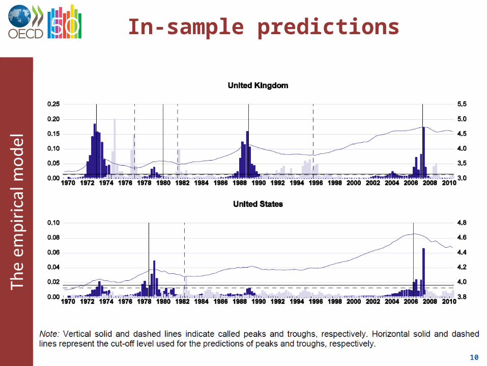
10

In-sample predictions

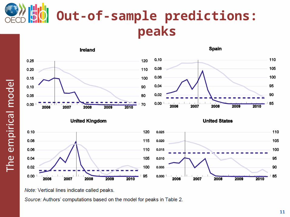
11

Out-of-sample predictions: peaks

12

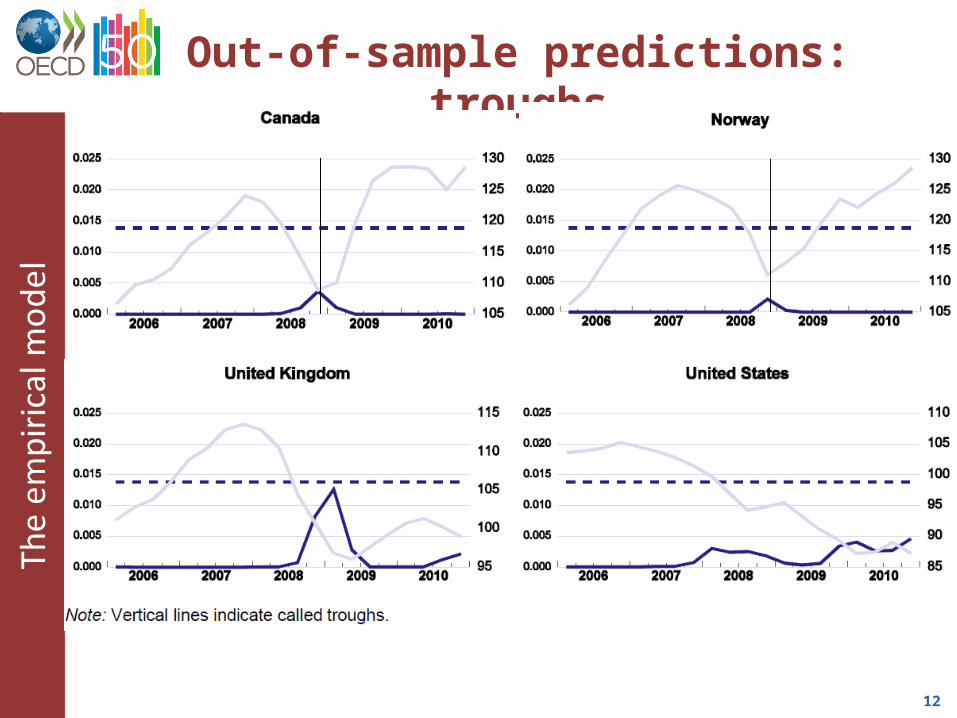
Out-of-sample predictions: troughs

13

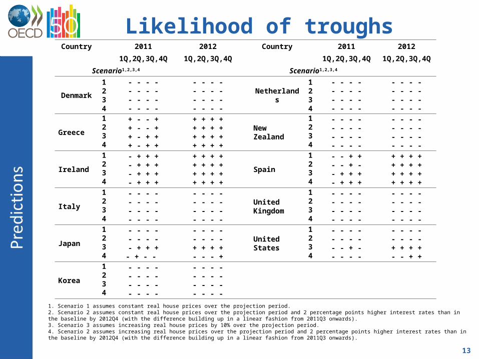
Likelihood of troughsCountry 2011 2012 Country 2011 2012

1Q,2Q,3Q,4Q 1Q,2Q,3Q,4Q 1Q,2Q,3Q,4Q 1Q,2Q,3Q,4Q

Scenario1,2,3,4 Scenario1,2,3,4

Denmark

1234

- - - -- - - -- - - -- - - -

- - - -- - - -- - - -- - - -

Netherlands

1234

- - - -- - - -- - - -- - - -

- - - -- - - -- - - -- - - -

Greece

1234

+ - - ++ - - ++ - + ++ - + +

+ + + ++ + + ++ + + ++ + + +

New Zealand

1234

- - - -- - - -- - - -- - - -

- - - -- - - -- - - -- - - -

Ireland

1234

- + + +- + + +- + + +- + + +

+ + + ++ + + ++ + + ++ + + +

Spain

1234

- - + +- - + -- + + +- + + +

+ + + ++ + + ++ + + ++ + + +

Italy

1234

- - - -- - - -- - - -- - - -

- - - -- - - -- - - -- - - -

United Kingdom

1234

- - - -- - - -- - - -- - - -

- - - -- - - -- - - -- - - -

Japan

1234

- - - -- - - -

- + + +- + - -

- - - -- - - -

+ + + +- - - +

United States

1234

- - - -- - - -- - + -- - - -

- - - -- - - -

+ + + +- - + +

Korea

1234

- - - -- - - -- - - -- - - -

- - - -- - - -- - - -- - - -

1. Scenario 1 assumes constant real house prices over the projection period.2. Scenario 2 assumes constant real house prices over the projection period and 2 percentage points higher interest rates than in the baseline by 2012Q4 (with the difference building up in a linear fashion from 2011Q3 onwards). 3. Scenario 3 assumes increasing real house prices by 10% over the projection period. 4. Scenario 2 assumes increasing real house prices over the projection period and 2 percentage points higher interest rates than in the baseline by 2012Q4 (with the difference building up in a linear fashion from 2011Q3 onwards).

14

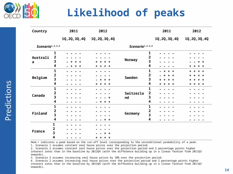
Likelihood of peaks

Country 2011 2012 2011 2012

1Q,2Q,3Q,4Q 1Q,2Q,3Q,4Q 1Q,2Q,3Q,4Q 1Q,2Q,3Q,4Q

Scenario1,2,3,4 Scenario1,2,3,4

Australia

1234

- - - -- - - -

- + + +- + + +

- - - -- - - -

+ + + ++ + + +

Norway

1234

- - - -- - - -- - - -- - - -

- - - -- - - -- - + ++ + + +

Belgium

1234

- - - -- - - -- - - -- - - -

- - - -- - - -

- + + ++ + + +

Sweden

1234

- + + +- + + ++ + + ++ + + +

+ + + ++ + + ++ + + ++ + + +

Canada

1234

- - - -- - - -- - - -- - - -

- - - -- - - -- - - +- + + +

Switzerland

1234

- - - -- - - -- - - -- - - -

- - - -- - - -- - - -- - - -

Finland

1234

- - - -- - - -- - - -- - - -

- - - -- - - -- - - -- - + +

Germany

1234

- - - -- - - -- - - -- - - -

- - - -- - - -- - - -- - - -

France

1234

- - - -- - - -- - - -- - - -

- - - -- - - -- - + ++ + + +

Note: + indicates a peak based on the cut-off level corresponding to the unconditional probability of a peak. 1. Scenario 1 assumes constant real house prices over the projection period.2. Scenario 2 assumes constant real house prices over the projection period and 2 percentage points higher interest rates than in the baseline by 2012Q4 (with the difference building up in a linear fashion from 2011Q3 onwards). 3. Scenario 3 assumes increasing real house prices by 10% over the projection period. 4. Scenario 2 assumes increasing real house prices over the projection period and 2 percentage points higher interest rates than in the baseline by 2012Q4 (with the difference building up in a linear fashion from 2011Q3 onwards).

15

Forecasts

Source: Authors’ calculations.

1.Downturns ending? United States*, United Kingdom†, Italy†, Denmark†, Greece**, Ireland**, Korea†, Netherlands†, New Zealand†, Spain**

2.Rebounds ending? France*, Canada*, Australia*, Belgium*, Finland*, Norway*, Sweden** ,Switzerland †

3.Long-term declines ending ? Japan* , Germany**

___________† No* Yes after a further fall (rise) in real

prices** Also at current real prices