1

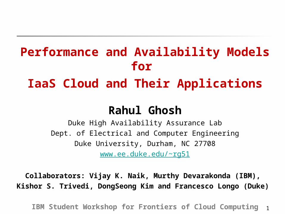
Performance and Availability Models for

IaaS Cloud and Their Applications

Rahul GhoshDuke High Availability Assurance Lab

Dept. of Electrical and Computer EngineeringDuke University, Durham, NC 27708

www.ee.duke.edu/~rg51

Collaborators: Vijay K. Naik, Murthy Devarakonda (IBM), Kishor S. Trivedi, DongSeong Kim and Francesco Longo (Duke)

IBM Student Workshop for Frontiers of Cloud ComputingHawthorne, NY, USASeptember 10, 2010

2

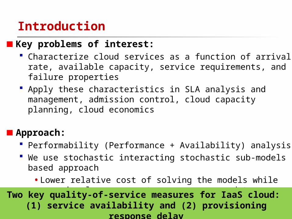
Key problems of interest: Characterize cloud services as a function of arrival rate,

available capacity, service requirements, and failure properties

Apply these characteristics in SLA analysis and management, admission control, cloud capacity planning, cloud economics

Approach: Performability (Performance + Availability) analysis We use stochastic interacting stochastic sub-models based

approach

•Lower relative cost of solving the models while covering large parameter space compared to measurement based analysis

Introduction

Two key quality-of-service measures for IaaS cloud: (1) service availability and (2) provisioning response

delay

3

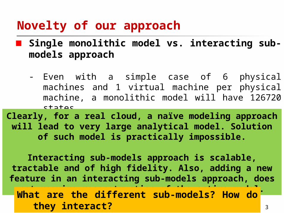
Novelty of our approachSingle monolithic model vs. interacting sub-models approach

- Even with a simple case of 6 physical machines and 1 virtual machine per physical machine, a monolithic model will have 126720 states.

- In contrast, our approach of interacting sub-models has only 41 states.

Clearly, for a real cloud, a naïve modeling approach will lead to very large analytical model. Solution of such

model is practically impossible.

Interacting sub-models approach is scalable, tractable and of high fidelity. Also, adding a new feature in an interacting sub-models approach, does not require

reconstruction of the entire model.What are the different sub-models? How do

they interact?

4

Main Assumptions All requests are homogenous, where each request is for one

virtual machine (VM) with fixed size CPU cores, RAM, disk capacity.

We use the term “job” to denote a user request for provisioning a VM.

Submitted requests are served in FCFS basis by resource provisioning decision engine (RPDE).

If a request can be accepted, it goes to a specific physical machine (PM) for VM provisioning. After getting the VM, the request runs in the cloud and releases the VM when it finishes.

To reduce cost of operations, PMs can be grouped into multiple pools. We assume three pools – hot (running with VM instantiated), warm (turned on but VM not instantiated) and cold (turned off).

All physical machines (PMs) in a particular type of pool are identical.

System model

5

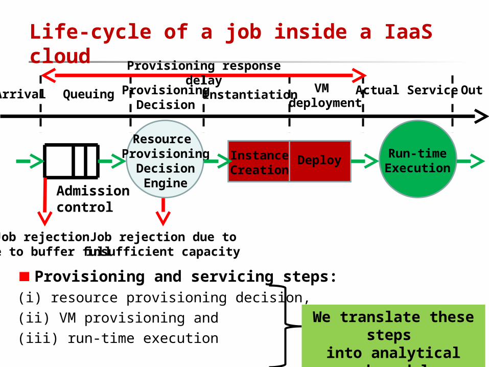
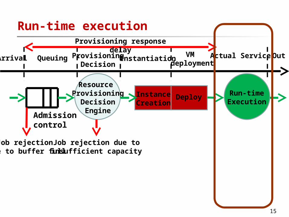
Provisioning and servicing steps:(i) resource provisioning decision, (ii) VM provisioning and (iii) run-time execution

Life-cycle of a job inside a IaaS cloud

We translate these steps

into analytical sub-models

Resource Provisioning

DecisionEngine

Run-timeExecution

InstanceCreation

Deploy

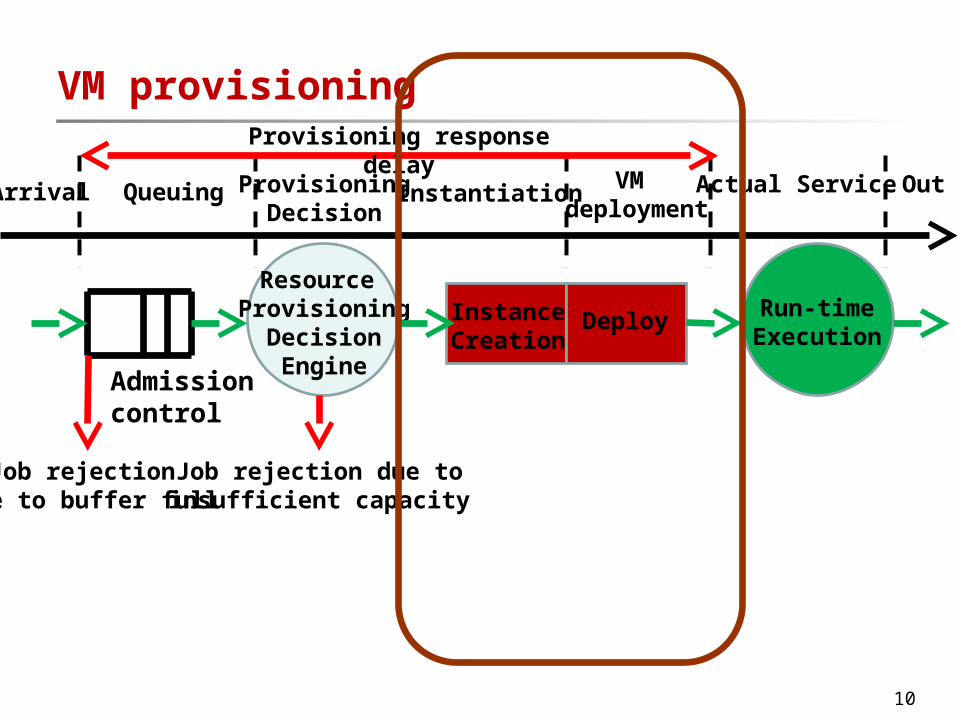
Job rejection due to buffer full

Job rejection due toinsufficient capacity

Arrival Queuing ProvisioningDecision

Instantiation VM deployment

Actual Service Out

Provisioning response delay

Admissioncontrol

6

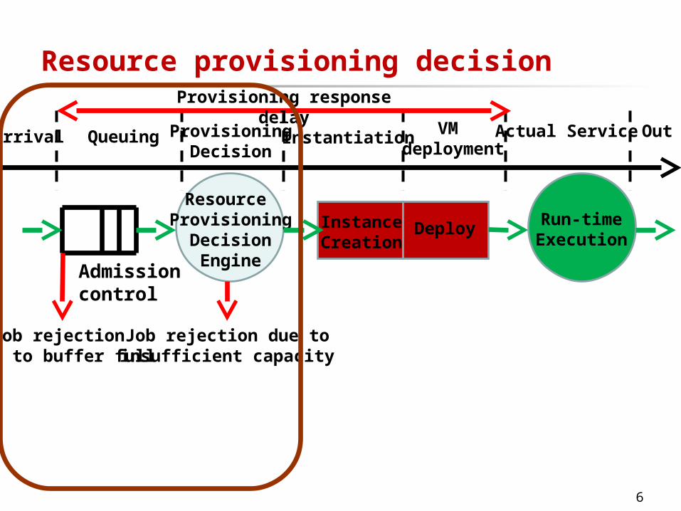
Resource provisioning decision

Resource Provisioning

DecisionEngine

Run-timeExecution

InstanceCreation

Deploy

Job rejection due to buffer full

Job rejection due toinsufficient capacity

Arrival Queuing ProvisioningDecision

Instantiation VM deployment

Actual Service Out

Provisioning response delay

Admissioncontrol

7

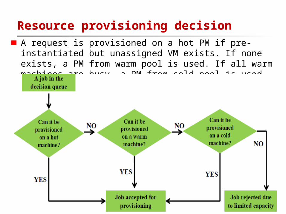
A request is provisioned on a hot PM if pre-instantiated but unassigned VM exists. If none exists, a PM from warm pool is used. If all warm machines are busy, a PM from cold pool is used.

Resource provisioning decision

8

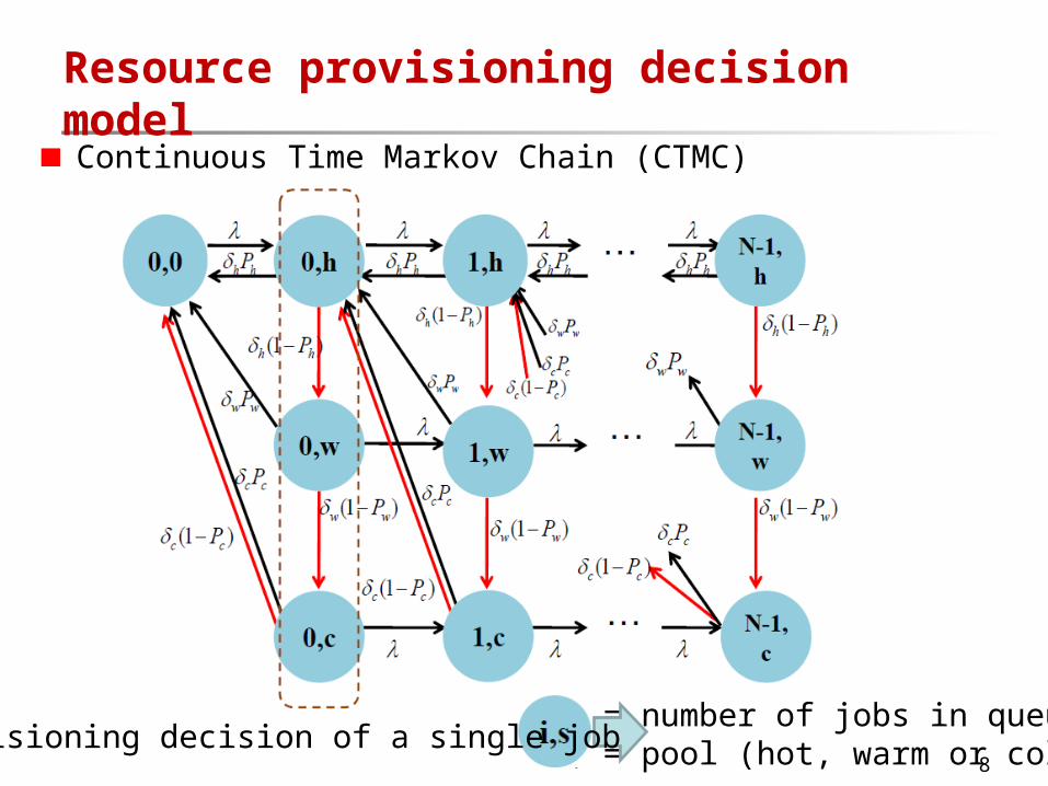
Continuous Time Markov Chain (CTMC)

Resource provisioning decision model

i = number of jobs in queue, s = pool (hot, warm or cold)Provisioning decision of a single job

9

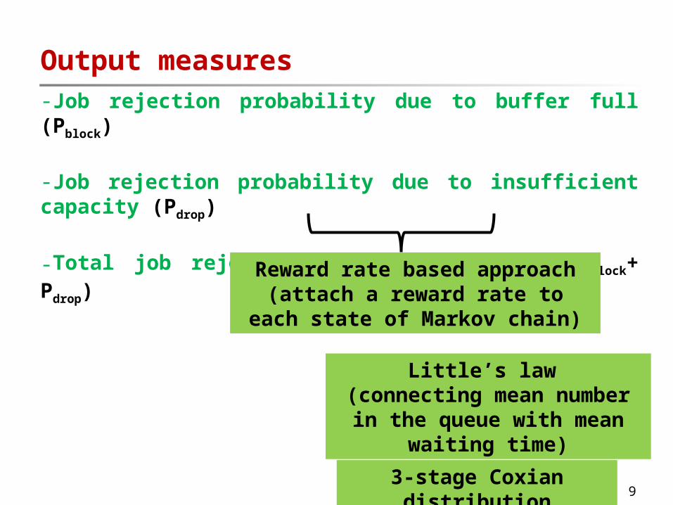
Output measures-Job rejection probability due to buffer full (Pblock)

-Job rejection probability due to insufficient capacity (Pdrop)

-Total job rejection probability (Preject= Pblock+ Pdrop)

-Mean queuing delay (E[Tq_dec])

-Mean decision delay (E[Tdecision])

Reward rate based approach(attach a reward rate to each

state of Markov chain)

Little’s law (connecting mean number

in the queue with mean waiting time)

3-stage Coxian distribution

10

VM provisioning

Resource Provisioning

DecisionEngine

Run-timeExecution

InstanceCreation

Deploy

Job rejection due to buffer full

Job rejection due toinsufficient capacity

Arrival Queuing ProvisioningDecision

Instantiation VM deployment

Actual Service Out

Provisioning response delay

Admissioncontrol

11

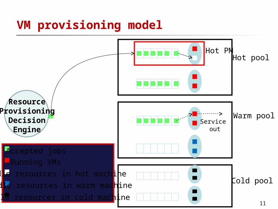
VM provisioning model

Service out

ResourceProvisioning

DecisionEngine

Accepted jobs

Running VMs

Idle resources in hot machine

Idle resources in warm machine

Idle resources in cold machine

Hot pool

Warm pool

Cold pool

Hot PM

12

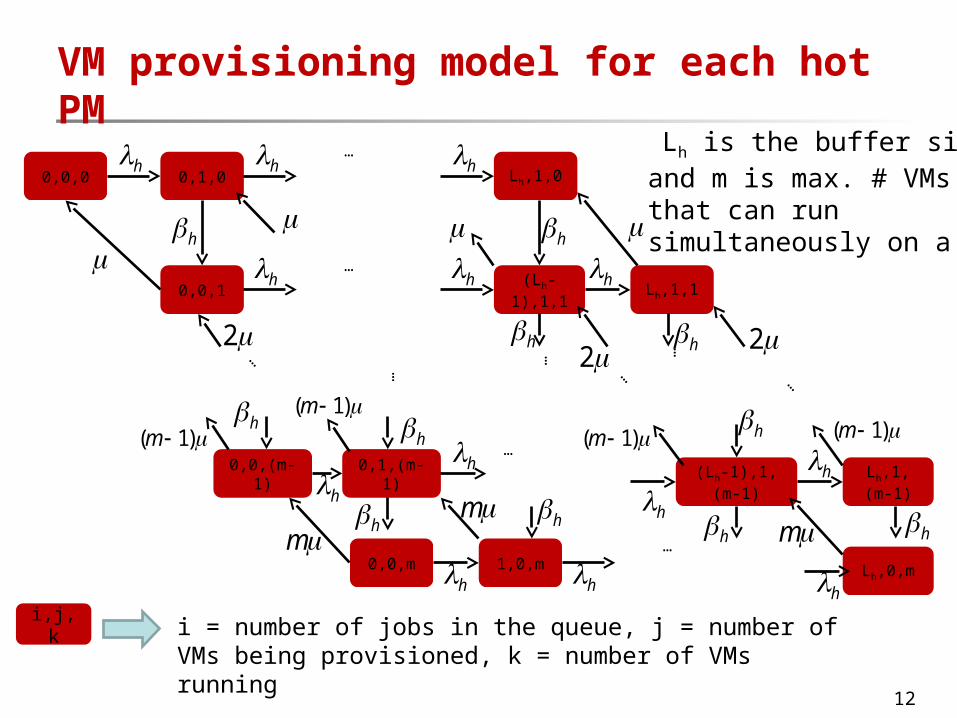
VM provisioning model for each hot PM

0,0,0 0,1,0 Lh,1,0

0,0,1(Lh-

1),1,1Lh,1,1

1,0,m Lh,0,m

Lh,1,(m-1)

0,0,m

(Lh-1),1,(m-1)

0,0,(m-1) 0,1,(m-1)

h h h

hh h

hh

hh

hhh

h h

hh h

hh

h hh h

22 2

)1( m

m

)1( m

mm

)1( m)1( m

…

…

…

…

…

… …

…

… …

Lh is the buffer sizeand m is max. # VMs that can run simultaneously on a PM

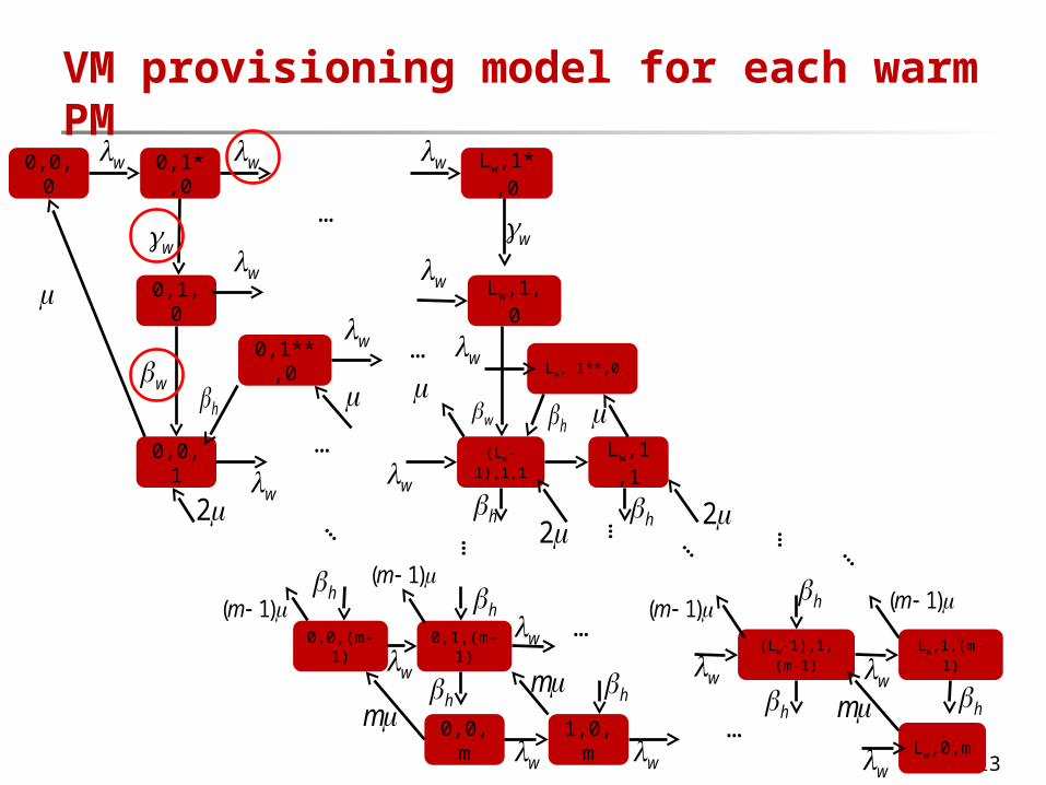
i,j,k i = number of jobs in the queue, j = number of VMs being provisioned, k = number of VMs running

13

VM provisioning model for each warm PM

0,0,00,1*,

0Lw,1*,

0

0,0,1(Lw-

1),1,1

Lw,1,1

w

w

hh

22 2

…

…

1,0,m Lw,0,m

Lw,1,(m-1)

0,0,m

(Lw-1),1,(m-1)

0,0,(m-1)

0,1,(m-1)

hh h

h hh h

)1( m

m

)1( m

mm

)1( m)1( m…

……

… …

…

… …

0,1,0 Lw,1,0

0,1**,0 Lw, 1**,0

w w

w ww w

whh

w…

w w

w

ww

w w

w w w

14

Output measures from VM provisioning models Prob. that a job can be accepted in the hot/warm/cold

pool (Ph /Pw /Pc)

Weighted mean queuing delay for VM provisioning (E[Tvm_q])

Weighted mean provisioning delay (E[Tprov])

15

Run-time execution

Resource Provisioning

DecisionEngine

Run-timeExecution

InstanceCreation

Deploy

Job rejection due to buffer full

Job rejection due toinsufficient capacity

Arrival Queuing ProvisioningDecision

Instantiation VM deployment

Actual Service Out

Provisioning response delay

Admissioncontrol

16

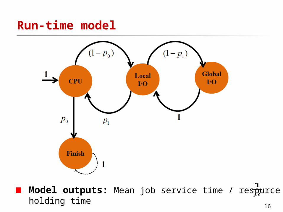
Run-time model

Model outputs: Mean job service time / resource holding time

1

17

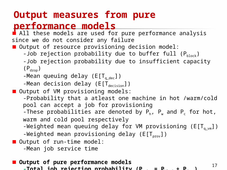
Output measures from pure performance models All these models are used for pure performance analysis since we do

not consider any failure Output of resource provisioning decision model:

-Job rejection probability due to buffer full (Pblock)-Job rejection probability due to insufficient capacity (Pdrop)-Mean queuing delay (E[Tq_dec])-Mean decision delay (E[Tdecision])

Output of VM provisioning models:-Probability that a atleast one machine in hot /warm/cold pool can accept a job for provisioning-These probabilities are denoted by Ph, Pw and Pc for hot, warm and cold pool respectively-Weighted mean queuing delay for VM provisioning (E[Tq_vm])-Weighted mean provisioning delay (E[Tprov])

Output of run-time model:-Mean job service time

Output of pure performance models-Total job rejection probability (Preject= Pblock + Pdrop)-Net mean response delay (E[Tresp]=E[Tq_dec]+E[Tdecision]+E[Tq_vm]+E[Tprov])

18

Availability model

Model outputs: Probability that the cloud service is available, downtime in minutes per year

19

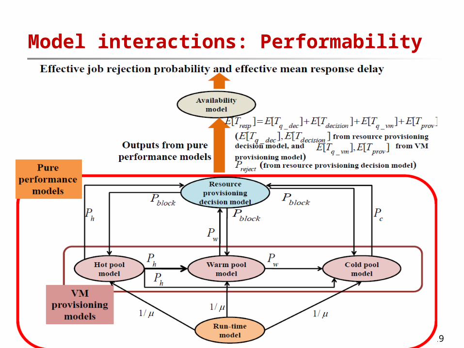
Model interactions: Performability

20

Numerical Results

21

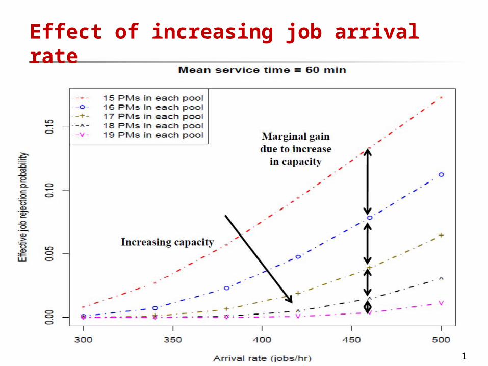
Effect of increasing job arrival rate

22

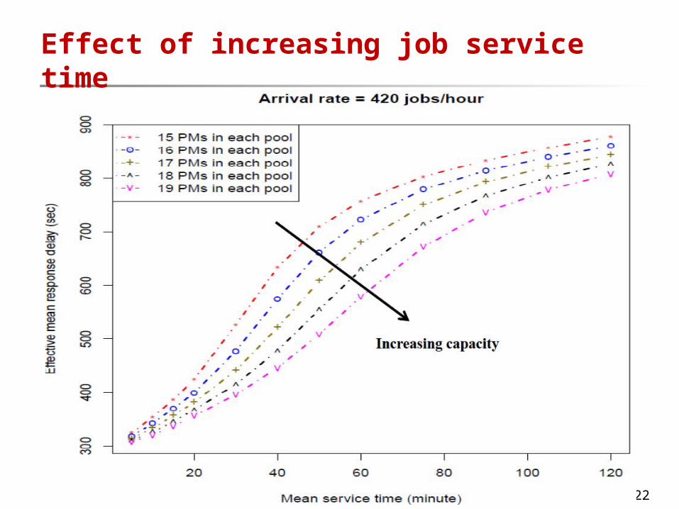
Effect of increasing job service time

23

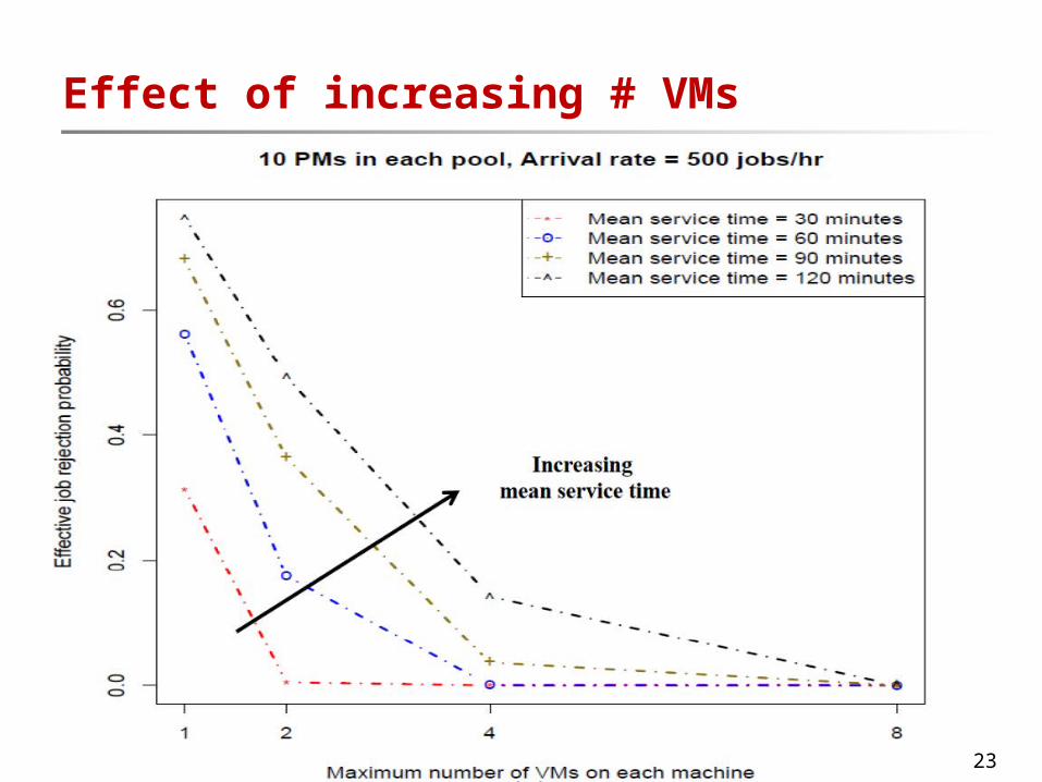
Effect of increasing # VMs

24

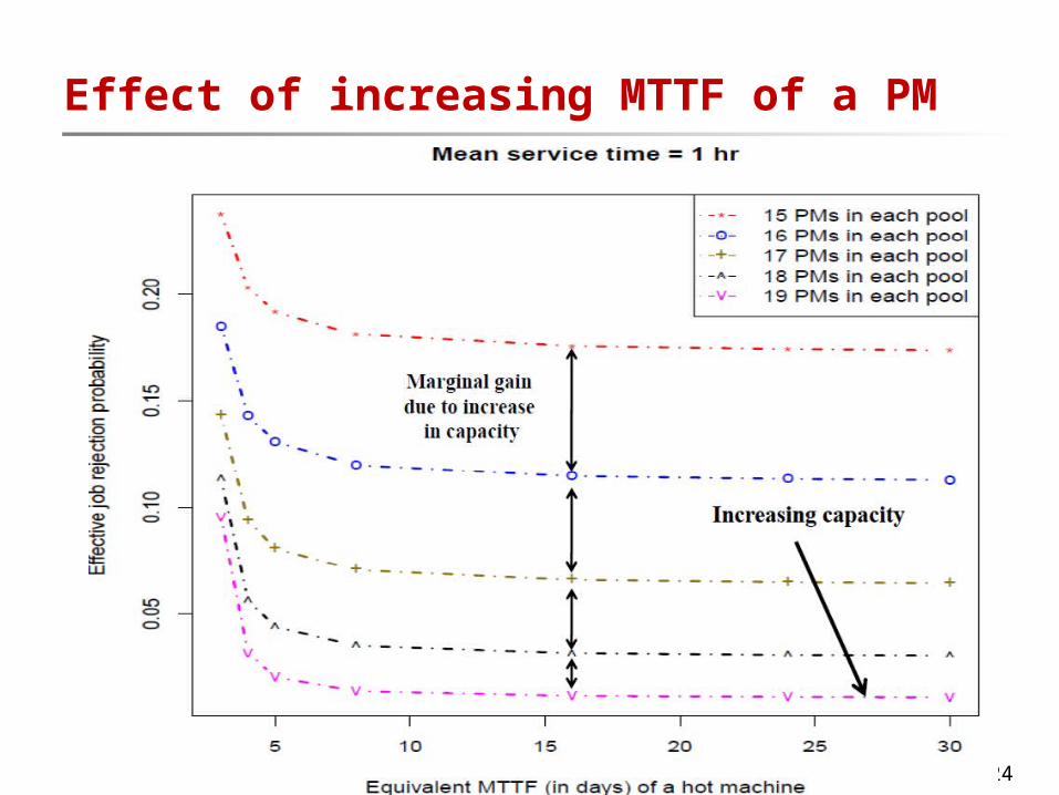
Effect of increasing MTTF of a PM

25

Applications of the models

26

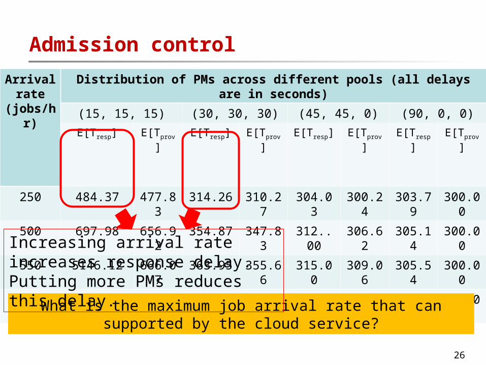
Admission control

Arrival rate

(jobs/hr)

Distribution of PMs across different pools (all delays are in seconds)

(15, 15, 15) (30, 30, 30) (45, 45, 0) (90, 0, 0)

E[Tresp] E[Tprov] E[Tresp] E[Tprov] E[Tresp] E[Tprov] E[Tresp] E[Tprov]

250 484.37 477.83

314.26 310.27

304.03 300.24

303.79

300.00

500 697.98 656.92

354.87 347.83

312..00

306.62

305.14

300.00

550 5146.12 666.07

363.95 355.66

315.00 309.06

305.54

300.00

600 13825.85 670.52

373.99 364.03

318.42 311.80

306.00

300.00

What is the maximum job arrival rate that can supported by the cloud service?

Increasing arrival rate increases response delay. Putting more PMs reduces this delay.

27

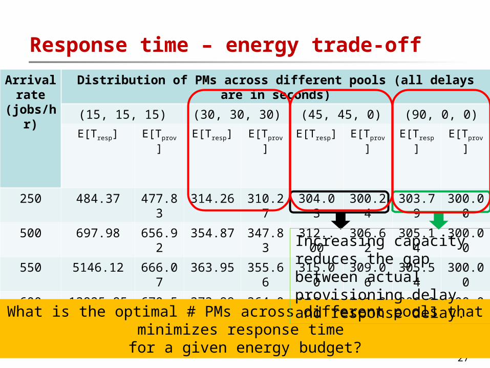
Response time – energy trade-off

Arrival rate

(jobs/hr)

Distribution of PMs across different pools (all delays are in seconds)

(15, 15, 15) (30, 30, 30) (45, 45, 0) (90, 0, 0)

E[Tresp] E[Tprov] E[Tresp] E[Tprov] E[Tresp] E[Tprov] E[Tresp] E[Tprov]

250 484.37 477.83

314.26 310.27

304.03 300.24

303.79

300.00

500 697.98 656.92

354.87 347.83

312..00

306.62

305.14

300.00

550 5146.12 666.07

363.95 355.66

315.00 309.06

305.54

300.00

600 13825.85 670.52

373.99 364.03

318.42 311.80

306.00

300.00What is the optimal # PMs across different pools that

minimizes response time for a given energy budget?

Increasing capacity reduces the gap between actual provisioning delay and response delay.

28

SLA driven capacity planning

What should be the size of each pool, so that total cost is minimized and SLA (maximum

rejection probability or response delay) is upheld?

29

Recent work on IaaS cloud resiliency

30

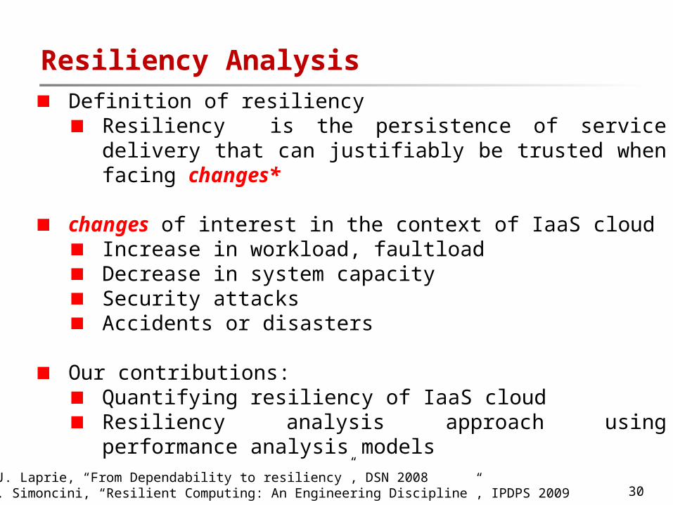
Resiliency Analysis Definition of resiliency

Resiliency is the persistence of service delivery that can justifiably be trusted when facing changes*

changes of interest in the context of IaaS cloudIncrease in workload, faultloadDecrease in system capacitySecurity attacksAccidents or disasters

Our contributions:Quantifying resiliency of IaaS cloudResiliency analysis approach using performance analysis models

*[1] J. Laprie, “From Dependability to resiliency”, DSN 2008[2] L. Simoncini, “Resilient Computing: An Engineering Discipline”, IPDPS 2009

31

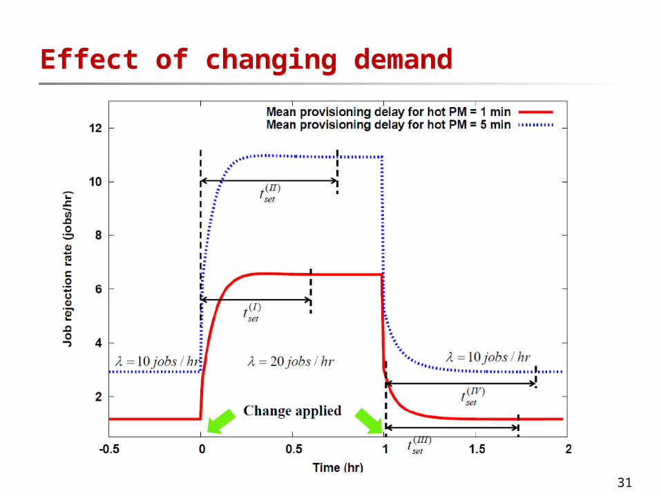
Effect of changing demand

32

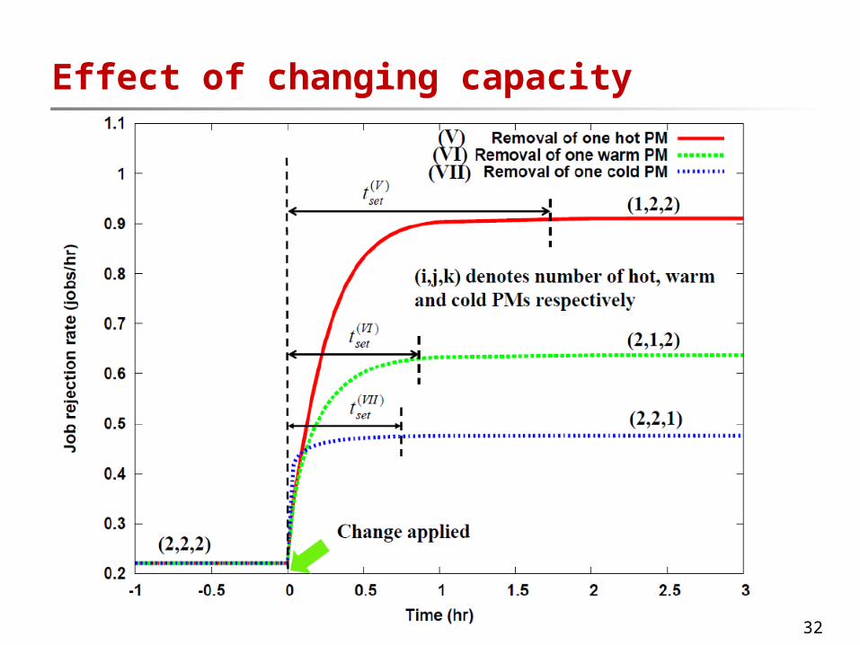
Effect of changing capacity

33

Conclusions Stochastic model can be an inexpensive alternative to

measurement based evaluation of cloud QoS

To reduce the complexity of modeling, we use an interacting sub-model approach

- Overall solution of the model is obtained iteration over individual sub-model solutions

The proposed approach is general and can be applicable to variety of IaaS clouds

Results show that IaaS cloud service quality is affected through variations in workload (job arrival rate, job service rate), faultload (machine failure rate) and available system capacity

This approach can be extended to solve specific cloud problems such as capacity planning of public, private and hybrid clouds

In future, models will be validated using real data collected from cloud

34

Thanks!