LEARNING OUTCOMES

1. Parallel and nonparallel shifts in the yield curve.

2. Factors that drive U.S. Treasury security returns.

3. Construct the theoretical spot rate curve.

4. The swap rate curve (LIBOR curve); why market participants have used the swap rate curve rather than a government bond yield curve as a benchmark.

5. Theories of the term structure of interest rates

(pure expectations, liquidity, and preferred habitat); the implications of each for the shape of the yield curve.

6. The yield curve risk and key rate duration.

7. Yield volatility.

• Parallel and nonparallel shifts in the yield curve

• Parallel Shift ← the yields on all maturities change in the same direction and by the same

amount (the slope of the yield curve remains unchanged).

• Nonparallel Shift ← the yields for the various maturities change by differing amounts (the

slope of the yield curve changed). • Nonparallel shifts fall into two general categories: Twists Shift and Butterfly Shift. • Flatting Twist Shift: the spread between short- and long term rates has narrowed:

• Steeping Twist Shift: the spread between short- and long term rates has widen:

• Positive Butterfly Shift: the yield curve has become less curved. For example, if rates

increase, the short and long maturity yields increase by more than the intermediate maturity yields.

• Negative Butterfly Shift: the yield curve has become more curved. For example, if rates increase, intermediate term yields increase by more than the long and short maturity yields.

• Factors that drive U.S. Treasury security returns

Three Factors : 1. Changes in the level of interest rates (parallel shifts in the yield curve). 2. Changes in the slope of the yield curve (twists in the yield curve). 3. Changes in the curvature of the yield curve (butterfly shifts).

• Factor 1: Changes in the level of rates made the greatest contribution, explaining almost 90% of the observed variation in total returns for all maturity levels.

• Factor 2: Slope changes explained, on average, 8.5% of the total returns’ variance over all maturity levels.

• Factor 3: Curvature changes contributed relatively little toward the explanation of total returns, with an average proportion of total explained variance equal to 1.5%.

NOTE:

• Because parallel changes in the level of interest rates (Factor 1) have a significant influence on Treasury returns, duration is a useful tool for quantifying interest rate risk.

• How to quantify bond price sensitivity to changes in the slope of the yield curve? Use Key Rate Duration.

• Construct the theoretical spot rate curve.

Four combinations of securities that can be used to construct a theoretical Treasury spot rate curve: (1) all on-the-run Treasury securities, (2) all on-the-run and some off-the-run Treasury securities, (3) all Treasury bonds, notes, and bills, and (4) Treasury strips. Why Spot Rates are so important? Suppose that the 7-year Treasury security you are interested in pricing has a coupon rate of 9%. If you look at the universe of 7-year Treasury securities, you will find that there are several different issues, each with different coupon rates. Which one is correct? →None of them are correct. In order to accurately price a fixed-income security, you need a spot rate for each cash flow. Thus, to value your 7-year 9% bond, you will need unique spot rates for each of the 14 coupon payments and a spot rate for the return of principal. In order to obtain all the necessary spot rates, you will need to construct a theoretical spot rate curve for Treasury securities. How to estimate Spot Rates? Treasury Bond Yields → Bootstrapping → Treasury Spot Rate Curve Example: Suppose that you know a 6-month U.S. Treasury bill has an annualized yield of 4% and a 1-year Treasury STRIP has an annualized yield of 4.5% (assume annual rates stated on a bond equivalent basis). Because these are both discount securities, the yields are spot rates. Given these spot rates, we can calculate the spot yield on a 1.5-year Treasury via bootstrapping. Assume that the 1.5-year Treasury is priced at $95 and carries a 4% coupon ($2 every six months). In this case, to calculate the 1.5-year spot rate, solve the following equation:

𝑃𝑟𝑖𝑐𝑒 = $2

�1 + 6 −𝑚𝑜𝑛𝑡ℎ 𝑆𝑃2 �

1 +$2

�1 + 12 −𝑚𝑜𝑛𝑡ℎ 𝑆𝑃2 �

2 +$102

�1 + 18 −𝑚𝑜𝑛𝑡ℎ 𝑆𝑃2 �

3

$95 = $2

(1.02)1 +$2

(1.0225)2 +$102

�1 + 18 −𝑚𝑜𝑛𝑡ℎ 𝑆𝑃2 �

3

So the 18-month Spot Rate = 7.66% Construct Spot Rate Curve (1) All On-the-Run Treasury Securities:

• The on-the-run issues have the largest trading volume and are, therefore, the most accurately priced issues.

• However, due to the tax effects on premium priced and discounted on-the-run coupon instruments, it is not appropriate to use the observed yield for these issues unless they are trading at par.

• Large maturity gaps exist after the 5-year note. • the yield that is necessary to make the issue trade at par must be computed. Using these

adjusted yields and filling in the missing maturities using linear extrapolation, an on-the-run yield curve (called the par coupon curve) can be constructed. The bootstrapping methodology can then be used to generate a theoretical spot rate curve.

(2) All On-the-Run and Some Off-the-Run Treasury Securities • Using just on-the-run issues creates problems because there aren’t on-the-run issues at every

maturity, which leaves large maturity gaps between the 5-year and longest maturities. To provide additional observed points on the par coupon curve, 20- and 25-year off-the-run issues are added to the on-the-run issues. Linear interpolation is used to estimate yields for missing on-the-run maturities, and bootstrapping is employed to generate the theoretical spot rate curve. Two problems with the “on-the-run plus selected issues” :

(1) Still doesn’t use all the rate information contained in Treasury issues (2) Rates may be distorted by the repo market

(3) All Treasury Coupon Securities and Bills • Bootstrapping is not useful in generating the theoretical spot rate curve when all Treasury securities

and bills are used, because more than one yield may exist for each maturity. • Current information about interest rates could be still unavailable for all issues.

(4) Treasury Strips • Note that the goal of the different yield curve construction approaches is to determine the spot

rates for all maturities. • Treasury coupon strips are zero-coupon securities made by stripping the coupons from normal T-

bonds. • Coupon strips are zero-coupon T-bonds, so their rates are expressed as spot rates—no

bootstrapping necessary. • The rates on strips are spot rates. • Main Problem: the strips market is not as liquid as the Treasury coupon market, so observed strip

rates include a liquidity premium.

The swap rate curve (LIBOR curve) • Suppose two parties might enter into a 2-year interest rate swap in which counterparty A

agrees to pay a fixed rate of 8% quarterly on a notional principal amount of $25 million, and counterparty B agrees to pay a floating rate equal to 3-month LIBOR on $25 million.

• The 8% fixed rate is called the 2-year swap rate. • The swap rate curve (also known as the LIBOR curve) is the series of swap rates quoted by

swap dealers over maturities extending from 2 to 30 years. • U.S. dollar LIBOR = the LIBOR curve specifically refers to swap rates in which one party pays

the fixed swap rate in U.S. dollars. • LIBOR-based swap spreads reflect only the credit risk of the counterparty, which is usually a

bank, so the swap curve is a AA-rated curve, not a default-free curve. • Why market participants tend to prefer the swap rate curve as a benchmark interest rate

curve rather than a government bond yield curve?

1. The swap market is not regulated by any government and makes swap rates in different countries more comparable.

2. Swap curves across countries are also more comparable because they reflect similar levels of credit risk, while government bond yield curves also reflect sovereign risk unique to each country.

3. The swap curve typically has yield quotes at 11 maturities between 2 and 30 years. The U.S. government bond yield curve, however, only has on-the-run issues trading at four maturities of at least two years (2-year, 5-year, 10-year, and 30-year).

Theories of the term structure of interest rates: A Review Pure (Unbiased) Expectations Theory

• Forward rates are solely a function of expected future spot rates. In other words, long-term interest rates equal the mean of future expected short-term rates.

• Suppose the 1-year spot rate is 5% and the 2-year spot rate is 7%. Under the pure expectations theory, the 1-year forward rate in one year must be 9%, because investing for two years at 7% yields approximately the same annual return as investing for the first year at 5% and the second year at 9%. In other words, the 2-year rate of 7% is the average of the expected future 1-year rates of 5% and 9%:

• The 9% rate in the previous example is called the implied forward rate:

1. Breakeven Rate: An investor would be indifferent between investing for two years at 7%, or investing at 5% for the first year and reinvesting in one year at the 9% breakeven rate.

2. The locked-in rate for some future period: invest in the 2-year bond instead of the 1-year bond, and essentially lock in a 9% rate for the 1-year period starting in one year.

3. It is the expected spot rate in one year.

Shortcoming of the pure expectations theory 1. Fail to recognize Price risk—the uncertainty associated with the future price of a bond that may be sold

prior to its maturity. 2. Fail to recognize Reinvestment risk—the uncertainty associated with the rate at which bond cash flows

can be reinvested over an investment horizon.

Liquidity Preference Theory

• Forward rates calculated from the pure expectations are biased estimates of the market’s expectation of future rates because they include a liquidity premium.

• Forward rates should reflect investors’ expectations of future spot rates plus a liquidity premium to compensate them for exposure to interest rate risk.

• Liquidity premium is in fact positively related to maturity • A positive-sloping yield curve may indicate that either: (1) the market expects future interest rates to

rise; or (2) that rates are expected to remain constant (or even fall), but the addition of the liquidity premium results in a positive slope.

• The size of the liquidity premiums need not be constant over time. They may be larger during periods of greater economic uncertainty, when risk aversion among investors is higher.

• Suppose the expected spot rate in the second year is only 8% (not 9%), and the 2-year spot rate is still 7%. The 2-year spot rate must be equal to the average of the 1-year rates plus a liquidity premium or

2-year spot rate = 7.0% = [(1.05×1.08)0.5 ̶-1]+ 2-year liquidity premium • 2-year liquidity premium = 7.0% ̶- 6.5% = 0.5%.

Preferred Habitat Theory

• Forward rates represent expected future spot rates plus a premium. • Premiums are related to supply and demand for funds at various maturities—not the term to maturity

(not necessarily a liquidity premium). • The existence of an imbalance between the supply and demand for funds in a given maturity range will

induce lenders and borrowers to shift from their preferred habitats (maturity range) to one that has the opposite imbalance.

• This theory can be used to explain almost any yield curve shape.

• Yield Curve Risk and Key Rate Duration

KEY RATE DURATION

• Measurement of the impact on nonparallel shifts in yield curve. • Note that tradition duration is defined as the sensitivity of the value of a security or

portfolio to changes in a single spot rate, holding all other spot rates constant. • But a fixed income security or their portfolio will have a duration for every point (maturity)

on the spot rate curve. That is, there is a set of (key) rate durations accompanies every security or portfolio.

• For example, the key rates of a 20-year bond might be 3 months, 1 year, 2 years, 3 years, 5 years, 7 years, 10 years, 15 years, and 20 years.

• A key rate duration is defined as the approximate percentage change in the value of a bond or bond portfolio in response to a 100 basis point change in the corresponding key rate, holding all other rates constant.

• Suppose there are four maturity points on the spot rate curve: the 2-year, 10-year, 20-year, and 25-year maturities, with key rate durations represented by D1, D2, D3, and D4, respectively. Also, assume that we have a portfolio of zero-coupon bonds with maturity and portfolio weights as follows:

Key Rate Duration Matrix

• The effective duration of a portfolio is the weighted average of the key rate durations of its individual security durations, where the weights are based on the market value portfolio weights. If the yield curve undergoes a parallel upward shift of 100 basis points, the value of the portfolio will decline by about 17.7 × 1.00% = 17.7%.

Using Key Rate Duration to Measure Yield Curve Risk

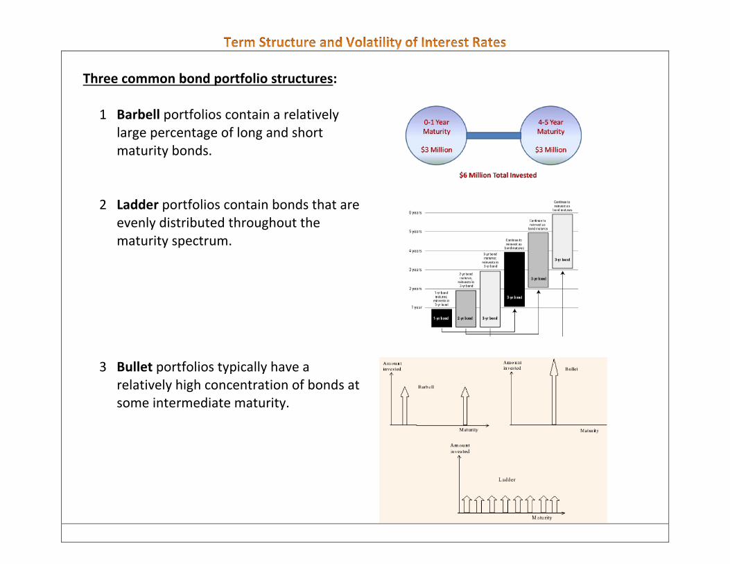
Three common bond portfolio structures:

1 Barbell portfolios contain a relatively large percentage of long and short maturity bonds.

2 Ladder portfolios contain bonds that are evenly distributed throughout the maturity spectrum.

3 Bullet portfolios typically have a relatively high concentration of bonds at some intermediate maturity.

• The portfolio duration for each structure is 9.63, implying that for a parallel shift in the yield curve, the

value of each of these portfolios will change by the same amount. For example, if the yield curve experiences a parallel downward shift of 75 basis points, the value of each portfolio will increase by approximately 9.63 ×0.75% = 7.22%.

• the 15-year key rate duration dominates all other key rate maturities for the bullet structure. The ladder portfolio’s key rate durations are fairly equal across all key rate maturities, and the barbell portfolio is characterized by relatively large key rate durations at the 3- and 25-year maturity levels.

• the impact of a 75 basis point increase in the 15-year spot rate while all other key rate maturity rates remain fairly stable. Because the bullet portfolio has the largest 15-year key rate duration, its value will decline more than the value of the ladder or barbell portfolios even though it has the same effective portfolio duration as the other two portfolios.

• The concept of key rate duration allows us to assess the impact of nonparallel shifts in the yield curve on the value of our portfolio. The sensitivity of a portfolio to any type of yield curve change can be evaluated with the key rate concept.