Embed Size (px)
Citation preview
CE 295 — Energy Systems and Control Professor Scott Moura — University of California, Berkeley
CHAPTER 3: OPTIMIZATION
1 Overview
Optimization is the process of maximizing or minimizing an objective function, subject to con-straints. Optimization is fundamental to nearly all academic fields, and its utility extends beyondenergy systems and control.
As energy systems engineers, we are often faced with design tasks. Here are some examples:
• Determine the optimal battery energy storage capacity for a wind farm [1].
• Optimally place x–MW of photovoltaic generation capacity in Nicaragua to minimize eco-nomic cost, yet meet consumer demand.
• Optimally place N vehicle sharing stations in an urban environment to optimally meet userdemand [2,3].
• Optimally re-distribute shared vehicles in a vehicle sharing system to minimize maintenancecost, yet serve user demand [4].
• Design an optimal plug-in electric vehicle charging strategy to minimize economic cost, yetmeet mobility demands and limit battery degradation [5].
• Optimally manage energy flow in a smart home, containing photovoltaics, battery storage,and a plug-in electric vehicle, to minimize economic cost [6].
• Optimally manage water flow in Barcelona’s water network to meet user demand, maintainsufficient quality, and minimize economic cost [7].
The number of interesting optimization examples in energy systems engineering is limited only byyour creativity. These problems often involve physical first principles of an energy storage/con-version device, user demand (a human element), and market economics. In addition, they arealmost always too complex to solve with pure intuition. Consequently, one desires a systematicprocess for designing energy systems that optimizes some metric of interest (e.g. economic costor performance), while satisfying some necessary constraints (e.g. user demand, physical oper-ating limits, regulations). In addition, we will find that optimization principles are the foundation ofmany machine learning concepts.
Revised February 28, 2018 | NOT FOR DISTRIBUTION Page 1
CE 295 — Energy Systems and Control Professor Scott Moura — University of California, Berkeley
1.1 Canonical Form
Nearly all static optimization problems can be abstracted into the following canonical form:
minimize f(x), (1)
subject to gi(x) ≤ 0, i = 1, · · · ,m (2)
hj(x) = 0, j = 1, · · · , l. (3)
In this formulation, x ∈ Rn is a vector of n decision variables. The function f(x) is known as the“cost function” or “objective function,” and maps the decision variables x into a scalar objectivefunction value, mathematically given by f(x) : Rn → R. Equation (2) represents m inequalityconstraints. Each function gi(x) maps the decision variable to a scalar that must be non-positivefor constraint satisfaction, mathematically gi(x) : Rn → R, ∀i = 1, · · · ,m. Similarly, equation (3)represents l equality constraints. Each function hi(x) maps the decision variable to a scalar thatmust be zero for constraint satisfaction, mathematically hj(x) : Rn → R,∀j = 1, · · · , l. We oftenvectorize the functions gi(x) and hj(x) as g(x) : Rn → Rm and h(x) : Rn → Rl, respectively, tomore compactly write the canonical form as:
minx
f(x) (4)
subject to g(x) ≤ 0, (5)
h(x) = 0. (6)
We denote by x? the solution that yields the smallest value of f(x) among all the values x thatsatisfy the constraints. That is, x? solves (1)-(3).
Remark 1.1. Note that one can always re-formulate a maximization problem, e.g. maxx f(x) intoa minimization problem by defining f(x) = −f(x) and solving minx f(x).
General optimization problems, without any structure beyond (1)-(3), are often very difficult tosolve. Namely, they lack analytical solutions and iterative methods involve tradeoffs. For example,one often sacrifices either long computation times, or not finding the exact solution. However,certain classes of (1)-(3) can be solved efficiently and reliably. Interestingly, huge swaths of prac-tical real-world problems fall within these classes of optimization problems. The crucial skill, then,becomes identifying these types of optimization problems in the real-world.
Several questions or issues arise:
1. What, exactly, is the definition of a minimum?
2. Does a solution even exist, and is it unique?
3. What are the different types of optimization problems?
Revised February 28, 2018 | NOT FOR DISTRIBUTION Page 2

CE 295 — Energy Systems and Control Professor Scott Moura — University of California, Berkeley
4. What are the properties of these optimization problems?
5. How do we solve optimization problems?
Throughout this chapter we shall investigate these questions in the context of energy applications.
1.2 Chapter Organization
The remainder of this chapter is organized as follows:
1. Mathematical Preliminaries
2. Linear Programs (LP)
3. Quadratic Programs (QP)
4. Convex Programs (CP)
5. Nonlinear Programs (NLP)
2 Mathematical Preliminaries
Our exposition of optimization begins with some important and useful mathematical concepts. Thisbackground will provide the necessary foundation to discuss the theory and algorithms underlyingvarious optimization problems. The first two concepts are convex sets and convex functions.
2.1 Convex Sets
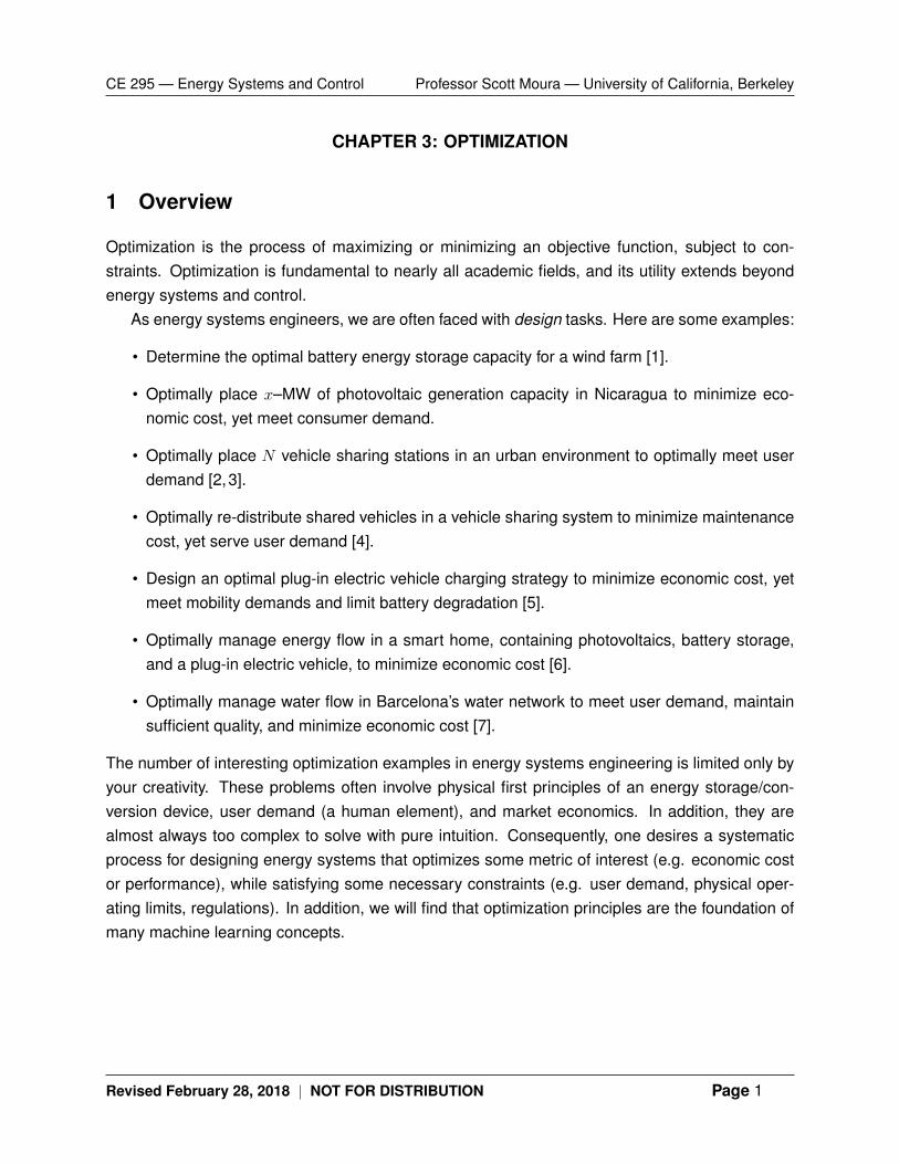
A set D is convex if the line segment connecting any two points in D completely lies in D. Weformalize this concept into the following definition.
Definition 2.1 (Convex Set). Let D be a subset of Rn. Also, consider scalar parameter λ ∈ [0, 1]
and two points a, b ∈ D. The set D is convex if
λa+ (1− λ)b ∈ D (7)
for all points a, b ∈ D.
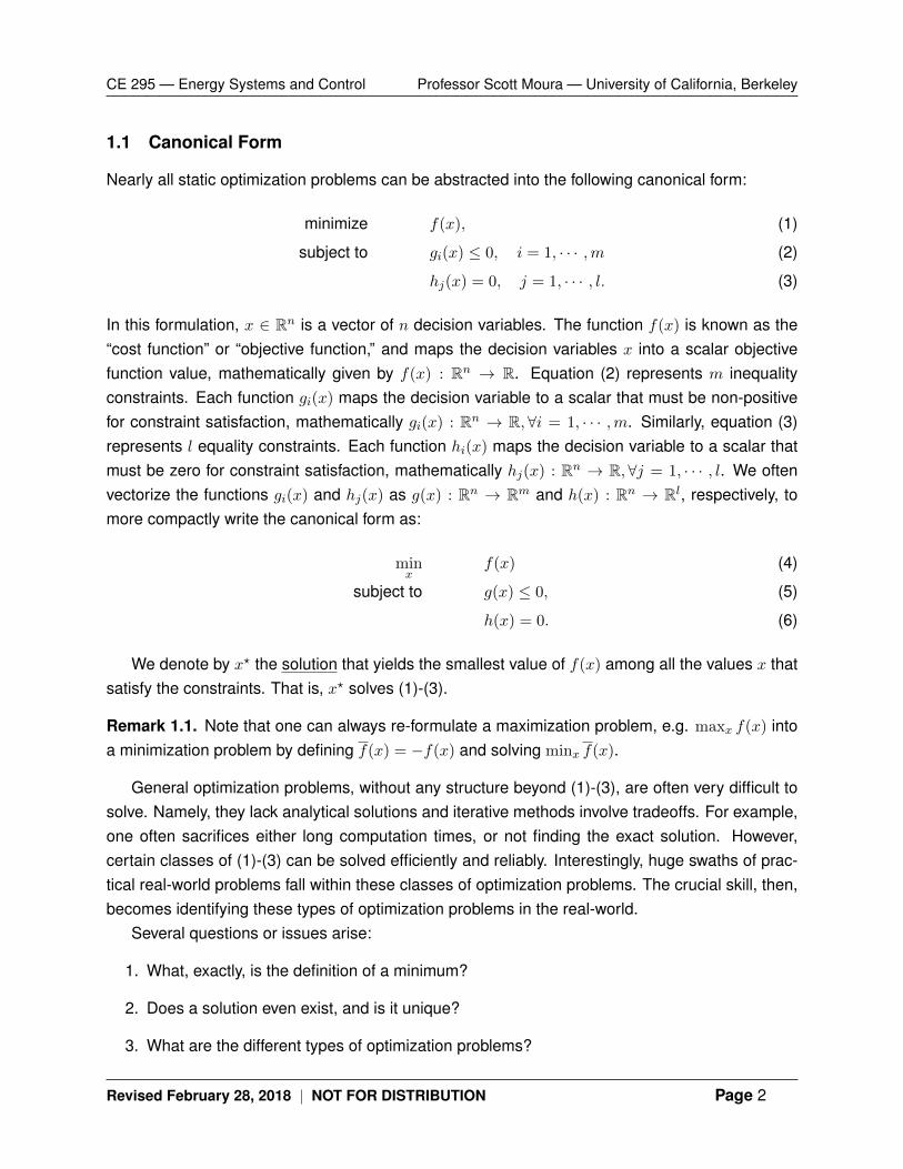
Figure 1 provides visualizations of convex and non-convex sets. In words, a set is convex if aline segment connecting any two points within domain D is completely within the set D. Figure 2provides additional examples of convex and non-convex sets.
Revised February 28, 2018 | NOT FOR DISTRIBUTION Page 3
CE 295 — Energy Systems and Control Professor Scott Moura — University of California, Berkeley
Figure 1: Visualization of convex [left] and non-convex [right] sets.
Figure 2: Some simple convex and nonconvex sets. [Left] The hexagon, which includes its boundary(shown darker), is convex. [Middle] The kidney shaped set is not convex, since the line segment betweenthe two points in the set shown as dots is not contained in the set. [Right] The square contains someboundary points but not others, and is not convex.
2.1.1 Examples
The following are some important examples of convex sets you will encounter in optimization:
• The empty set , any single point (i.e. a singleton), {x0}, and the whole space Rn are convex.
• Any line in Rn is convex.
• Any line segment in Rn is convex.
• A ray, which has the form {x0 + θv | θ ≥ 0, v 6= 0} is convex.
• A hyperplane, which has the form{x | aTx = b
}, where a ∈ Rn, a 6= 0, b ∈ R.
• A halfspace, which has the form{x | aTx ≤ b
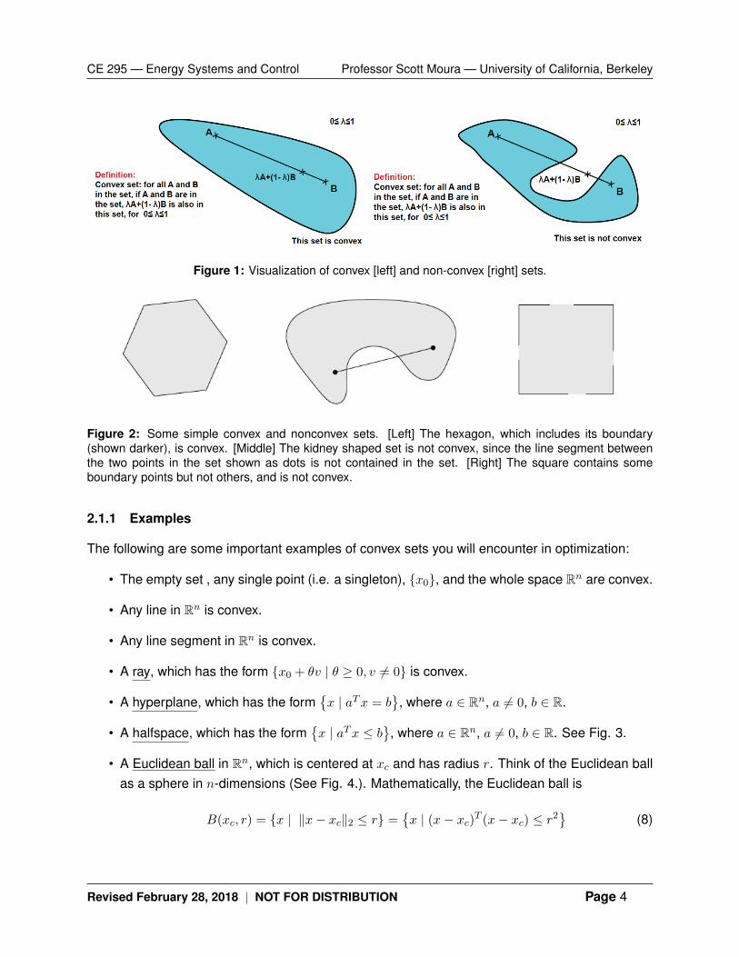
}, where a ∈ Rn, a 6= 0, b ∈ R. See Fig. 3.
• A Euclidean ball in Rn, which is centered at xc and has radius r. Think of the Euclidean ballas a sphere in n-dimensions (See Fig. 4.). Mathematically, the Euclidean ball is
B(xc, r) = {x | ‖x− xc‖2 ≤ r} ={x | (x− xc)T (x− xc) ≤ r2
}(8)
Revised February 28, 2018 | NOT FOR DISTRIBUTION Page 4
CE 295 — Energy Systems and Control Professor Scott Moura — University of California, Berkeley
x0
a
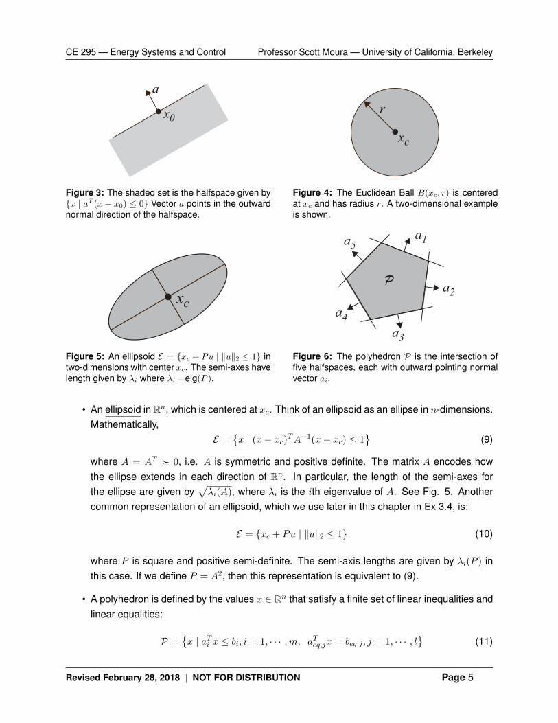
Figure 3: The shaded set is the halfspace given by{x | aT (x− x0) ≤ 0} Vector a points in the outwardnormal direction of the halfspace.
xc
r
Figure 4: The Euclidean Ball B(xc, r) is centeredat xc and has radius r. A two-dimensional exampleis shown.
xc
Figure 5: An ellipsoid E = {xc + Pu | ‖u‖2 ≤ 1} intwo-dimensions with center xc. The semi-axes havelength given by λi where λi =eig(P ).
P
a1
a2
a3
a4
a5
Figure 6: The polyhedron P is the intersection offive halfspaces, each with outward pointing normalvector ai.
• An ellipsoid in Rn, which is centered at xc. Think of an ellipsoid as an ellipse in n-dimensions.Mathematically,
E ={x | (x− xc)TA−1(x− xc) ≤ 1
}(9)
where A = AT � 0, i.e. A is symmetric and positive definite. The matrix A encodes howthe ellipse extends in each direction of Rn. In particular, the length of the semi-axes forthe ellipse are given by
√λi(A), where λi is the ith eigenvalue of A. See Fig. 5. Another
common representation of an ellipsoid, which we use later in this chapter in Ex 3.4, is:
E = {xc + Pu | ‖u‖2 ≤ 1} (10)
where P is square and positive semi-definite. The semi-axis lengths are given by λi(P ) inthis case. If we define P = A2, then this representation is equivalent to (9).
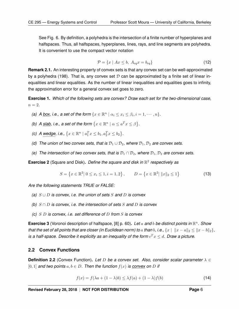
• A polyhedron is defined by the values x ∈ Rn that satisfy a finite set of linear inequalities andlinear equalities:
P ={x | aTi x ≤ bi, i = 1, · · · ,m, aTeq,jx = beq,j , j = 1, · · · , l
}(11)
Revised February 28, 2018 | NOT FOR DISTRIBUTION Page 5
CE 295 — Energy Systems and Control Professor Scott Moura — University of California, Berkeley
See Fig. 6. By definition, a polyhedra is the intersection of a finite number of hyperplanes andhalfspaces. Thus, all halfspaces, hyperplanes, lines, rays, and line segments are polyhedra.It is convenient to use the compact vector notation
P = {x | Ax ≤ b, Aeqx = beq} (12)
Remark 2.1. An interesting property of convex sets is that any convex set can be well-approximatedby a polyhedra (198). That is, any convex set D can be approximated by a finite set of linear in-equalities and linear equalities. As the number of linear inequalities and equalities goes to infinity,the approximation error for a general convex set goes to zero.
Exercise 1. Which of the following sets are convex? Draw each set for the two-dimensional case,n = 2.
(a) A box, i.e., a set of the form {x ∈ Rn | αi ≤ xi ≤ βi, i = 1, · · · , n}.
(b) A slab, i.e., a set of the form{x ∈ Rn | α ≤ aTx ≤ β
}.
(c) A wedge, i.e.,{x ∈ Rn | aT1 x ≤ b1, aT2 x ≤ b2
}.
(d) The union of two convex sets, that is D1 ∪ D2, where D1,D2 are convex sets.
(e) The intersection of two convex sets, that is D1 ∩ D2, where D1,D2 are convex sets.
Exercise 2 (Square and Disk). Define the square and disk in R2 respectively as
S ={x ∈ R2| 0 ≤ xi ≤ 1, i = 1, 2
}, D =
{x ∈ R2| ‖x‖2 ≤ 1
}(13)
Are the following statements TRUE or FALSE:
(a) S ∪D is convex, i.e. the union of sets S and D is convex
(b) S ∩D is convex, i.e. the intersection of sets S and D is convex
(c) S D is convex, i.e. set difference of D from S is convex
Exercise 3 (Voronoi description of halfspace, [8] p. 60). Let a and b be distinct points in Rn. Showthat the set of all points that are closer (in Euclidean norm) to a than b, i.e., {x | ‖x− a‖2 ≤ ‖x− b‖2},is a half-space. Describe it explicitly as an inequality of the form cTx ≤ d. Draw a picture.
2.2 Convex Functions
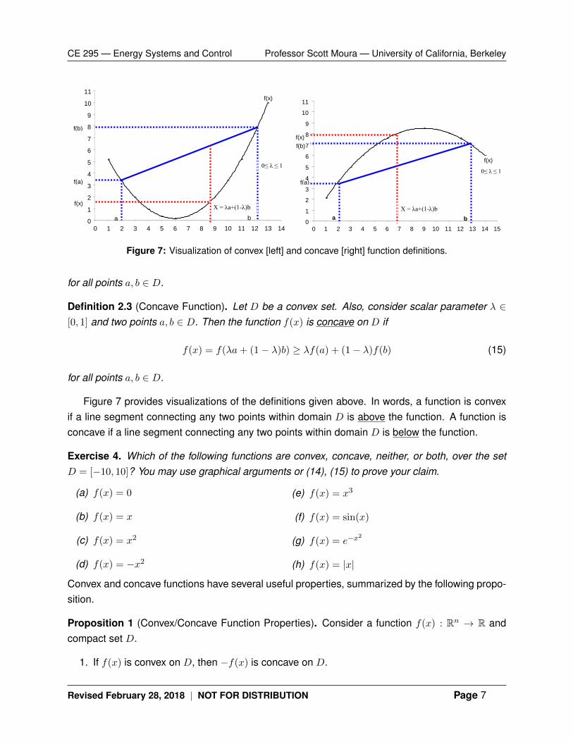
Definition 2.2 (Convex Function). Let D be a convex set. Also, consider scalar parameter λ ∈[0, 1] and two points a, b ∈ D. Then the function f(x) is convex on D if
f(x) = f(λa+ (1− λ)b) ≤ λf(a) + (1− λ)f(b) (14)
Revised February 28, 2018 | NOT FOR DISTRIBUTION Page 6
CE 295 — Energy Systems and Control Professor Scott Moura — University of California, Berkeley
Figure 1: Convex Function
Figure 2: Concave Function
b a
f(x)
f(b)
f(a)
f(x)
0
1
2
3
4
5
6
7
8
9
10
11
0 1 2 3 4 5 6 7 8 9 10 11 12 13 14
0≤ λ ≤ 1
X = λa+(1-λ)b
f(a)
f(b)
f(x)
a b
f(x)
0
1
2
3
4
5
6
7
8
9
10
11
0 1 2 3 4 5 6 7 8 9 10 11 12 13 14 15
0≤ λ ≤ 1
X = λa+(1-λ)b
Figure 1: Convex Function
Figure 2: Concave Function
b a
f(x)
f(b)
f(a)
f(x)
0
1
2
3
4
5
6
7
8
9
10
11
0 1 2 3 4 5 6 7 8 9 10 11 12 13 14
0≤ λ ≤ 1
X = λa+(1-λ)b
f(a)
f(b)
f(x)
a b
f(x)
0
1
2
3
4
5
6
7
8
9
10
11
0 1 2 3 4 5 6 7 8 9 10 11 12 13 14 15
0≤ λ ≤ 1
X = λa+(1-λ)b
Figure 7: Visualization of convex [left] and concave [right] function definitions.
for all points a, b ∈ D.
Definition 2.3 (Concave Function). Let D be a convex set. Also, consider scalar parameter λ ∈[0, 1] and two points a, b ∈ D. Then the function f(x) is concave on D if
f(x) = f(λa+ (1− λ)b) ≥ λf(a) + (1− λ)f(b) (15)
for all points a, b ∈ D.
Figure 7 provides visualizations of the definitions given above. In words, a function is convexif a line segment connecting any two points within domain D is above the function. A function isconcave if a line segment connecting any two points within domain D is below the function.
Exercise 4. Which of the following functions are convex, concave, neither, or both, over the setD = [−10, 10]? You may use graphical arguments or (14), (15) to prove your claim.
(a) f(x) = 0
(b) f(x) = x
(c) f(x) = x2
(d) f(x) = −x2
(e) f(x) = x3
(f) f(x) = sin(x)
(g) f(x) = e−x2
(h) f(x) = |x|
Convex and concave functions have several useful properties, summarized by the following propo-sition.
Proposition 1 (Convex/Concave Function Properties). Consider a function f(x) : Rn → R andcompact set D.
1. If f(x) is convex on D, then −f(x) is concave on D.
Revised February 28, 2018 | NOT FOR DISTRIBUTION Page 7
CE 295 — Energy Systems and Control Professor Scott Moura — University of California, Berkeley
2. If f(x) is concave on D, then −f(x) is convex on D.
3. f(x) is a convex function on D ⇐⇒ d2fdx2
(x) is positive semi-definite ∀ x ∈ D.
4. f(x) is a concave function on D ⇐⇒ d2fdx2
(x) is negative semi-definite ∀ x ∈ D.
2.2.1 Examples
It is easy to verify that all linear and affine functions are both convex and concave functions.Here we provide more interesting examples of convex and concave functions. First, we considerfunctions f(x) where x ∈ R is scalar.
• Quadratic. 12ax
2 + bx+ c is convex on R, for any a ≥ 0. It is concave on R for any a ≤ 0.
• Exponential. eax is convex on R, for any a ∈ R.
• Powers. xa is convex on the set of all positive x, when a ≥ 1 or a ≤ 0. It is concave for0 ≤ a ≤ 1.
• Powers of absolute value. |x|p, for p ≥ 1 is convex on R.
• Logarithm. log x is concave on the set of all positive x.
• Negative entropy. x log x is convex on the set of all positive x.
Convexity or concavity of these examples can be shown by directly verifying (14), (15), or bychecking that the second derivative is non-negative (degenerate of positive semi-definite) or non-positive (degenerate of negative semi-definite). For example, with f(x) = x log x we have
f ′(x) = log x+ 1, f ′′(x) = 1/x,
so that f ′′(x) ≥ 0 for x > 0. Therefore the negative entropy function is convex for positive x.We now provide a few commonly used examples in the multivariable case of f(x), where
x ∈ Rn.
• Norms. Every norm in Rn is convex.
• Max function. f(x) = max{x1, · · · , xn} is convex on Rn.
• Quadratic-over-linear function. The function f(x, y) = x2/y is convex over x ∈ R, y > 0.
• Log-sum-exp. The function f(x) = log (expx1 + · · ·+ expxn) is convex on Rn. This functioncan be interpreted as a differentiable (in fact, analytic) approximation of the max function.Consequently, it is extraordinarily useful for gradient-based algorithms, such as the onesdescribed in Section 4.1.
Revised February 28, 2018 | NOT FOR DISTRIBUTION Page 8
CE 295 — Energy Systems and Control Professor Scott Moura — University of California, Berkeley
• Geometric mean. The geometric mean f(x) = (Πni=1xi)
1/n is concave for all elements of xpositive, i.e. {x ∈ Rn | xi > 0 ∀ i = 1, · · · , n}.
• Log determinant. The function f(X) = log det(X) is concave w.r.t. X for all X positivedefinite. This property is useful in many applications, including optimal experiment design.
Convexity (or concavity) of these examples can be shown by directly verifying (14), (15), or bychecking that the Hessian is positive semi-definite (or negative semi-definite). These are left asexercises for the reader.
2.2.2 Operations that conserve convexity
Next we describe operations on convex functions that preserve convexity. These operations in-clude addition, scaling, and point-wise maximum. Often, objective functions in the optimal designof engineering system are a combination of convex functions via these operations. This sectionhelps you analyze when the combination is convex, and how to construct new convex functions.
Linear Combinations
It is easy to verify from (14) that when f(x) is a convex function, and α ≥ 0, then the functionαf(x) is convex. Similarly, if f1(x) and f2(x) are convex functions, then their sum f1(x) + f2(x) isa convex function. Combining non-negative scaling and addition yields a non-negative weightedsum of convex functions
f(x) = α1f1(x) + · · ·+ αmfm(x) (16)
that is also convex.
Pointwise Maximum
If f1(x) and f2(x) are convex functions on D, then their point-wise maximum f defined by
f(x) = max{f1(x), f2(x)} (17)
is convex on D. This property can be verified via (14) by considering 0 ≤ λ ≤ 1 and a, b ∈ D.
f(λa+ (1− λ)b) = max {f1(λa+ (1− λ)b), f2(λa+ (1− λ)b)}
≤ max {λf1(a) + (1− λ)f1(b), λf2(a) + (1− λ)f2(b)}
≤ λmax {f1(a), f2(a)}+ (1− λ) max {f1(b), f2(b)}
= λf(a) + (1− λ)f(b).
Revised February 28, 2018 | NOT FOR DISTRIBUTION Page 9
CE 295 — Energy Systems and Control Professor Scott Moura — University of California, Berkeley
which establishes convexity of f . It is straight-forward to extend this result to show that if f1(x), · · · , fm(x)
are convex, then their point-wise maximum
f(x) = max{f1(x), · · · , fm(x)} (18)
is also convex.
Composition with an Affine Mapping
Consider f(·) : Rn → R with parameters A ∈ Rn×m and b ∈ Rn. Define function g(·) : Rm → R as
g(x) = f(Ax+ b) (19)
If f is convex, then g is convex. If f is concave, then g is concave.
Exercise 5 (Simple function compositions). Consider function g(·) : R → R defined over convexset D. Prove each of the following function compositions is convex or concave over D.
(a) If g is convex, then exp g(x) is convex.
(b) If g is concave and positive, then log g(x) is concave.
(c) If g is concave and positive, then 1/g(x) is convex.
(d) If g is convex and nonnegative and p ≥ 1, then g(x)p is convex.
(e) If g is convex then − log(−g(x)) is convex on {x|g(x) < 0}.
2.3 Definition of Minimizers
Armed with notions of convex sets and convex/concave functions, we are positioned to provide aprecise definition of a minimizer, which we often denote with the “star” notation as x∗. There existtwo types of minimizers: global and local minimizers. Their definitions are given as follows.
Definition 2.4 (Global Minimizer). x∗ ∈ D is a global minimizer of f(x) on D if
f(x∗) ≤ f(x), ∀ x ∈ D (20)
In words, this means x∗ minimizes f(x) everywhere in D. In contrast, we have a local minimizer.
Definition 2.5 (Local Minimizer). x∗ ∈ D is a local minimizer of f(x) on D if
∃ ε > 0 s.t. f(x∗) ≤ f(x), ∀ x ∈ D ∩ {x ∈ R | ‖x− x∗‖ < ε} (21)
Revised February 28, 2018 | NOT FOR DISTRIBUTION Page 10
CE 295 — Energy Systems and Control Professor Scott Moura — University of California, Berkeley
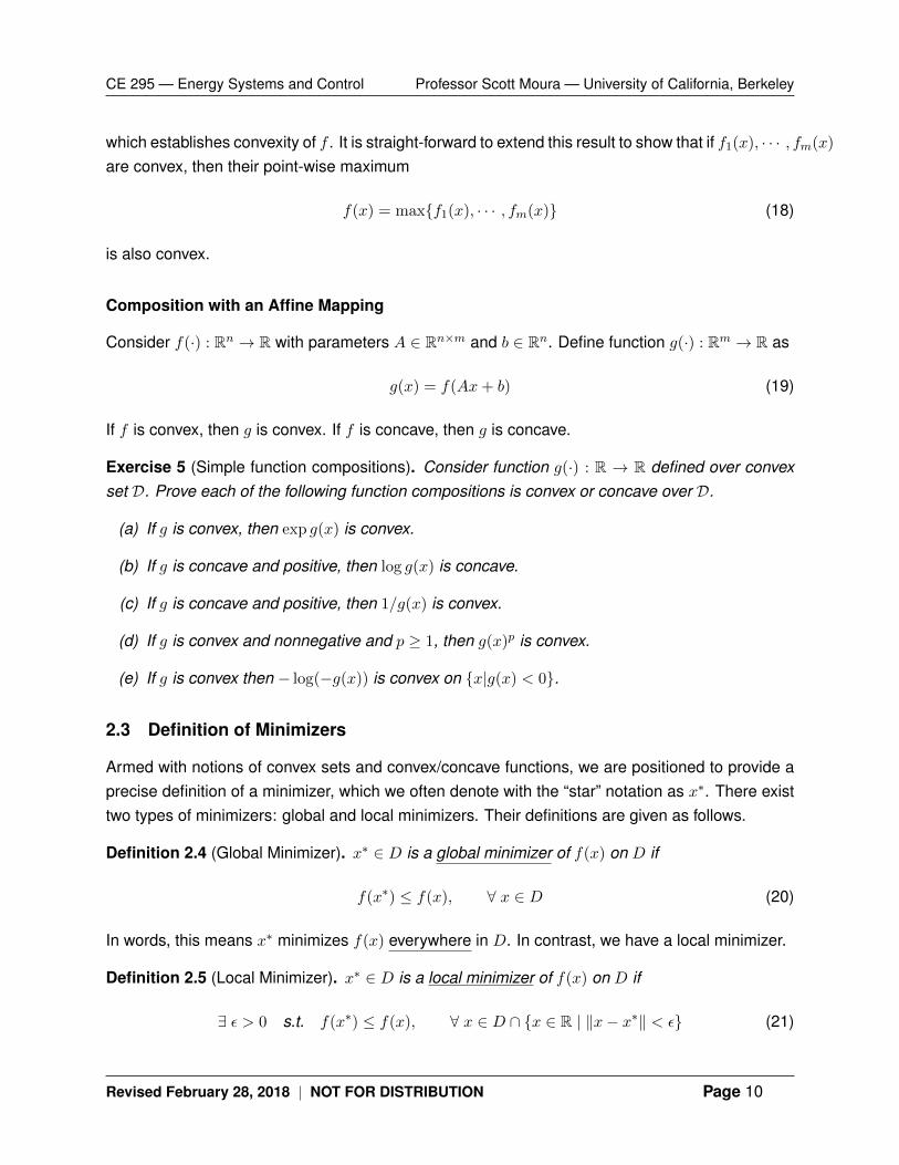
In words, this means x∗ minimizes f(x) locally in D. That is, there exists some neighborhoodwhose size is characterized by εwhere x∗ minimizes f(x). Examples of global and local minimizersare provided in Fig. 8
Figure 8: The LEFT figure contains two local minimizers, but only one global minimizer. The RIGHT figurecontains a local minimizer, which is also the global minimizer.
We now have a precise definition for a minimum. However, we now seek to understand whena minimum even exists. The answer to this question leverages the convex set notion, and is calledthe Weierstrauss Extreme Value Theorem.
Theorem 2.1 (Weierstrass Extreme Value Theorem). If f(x) is continuous and bounded on aconvex set D, then there exists at least one global minimum of f on D.
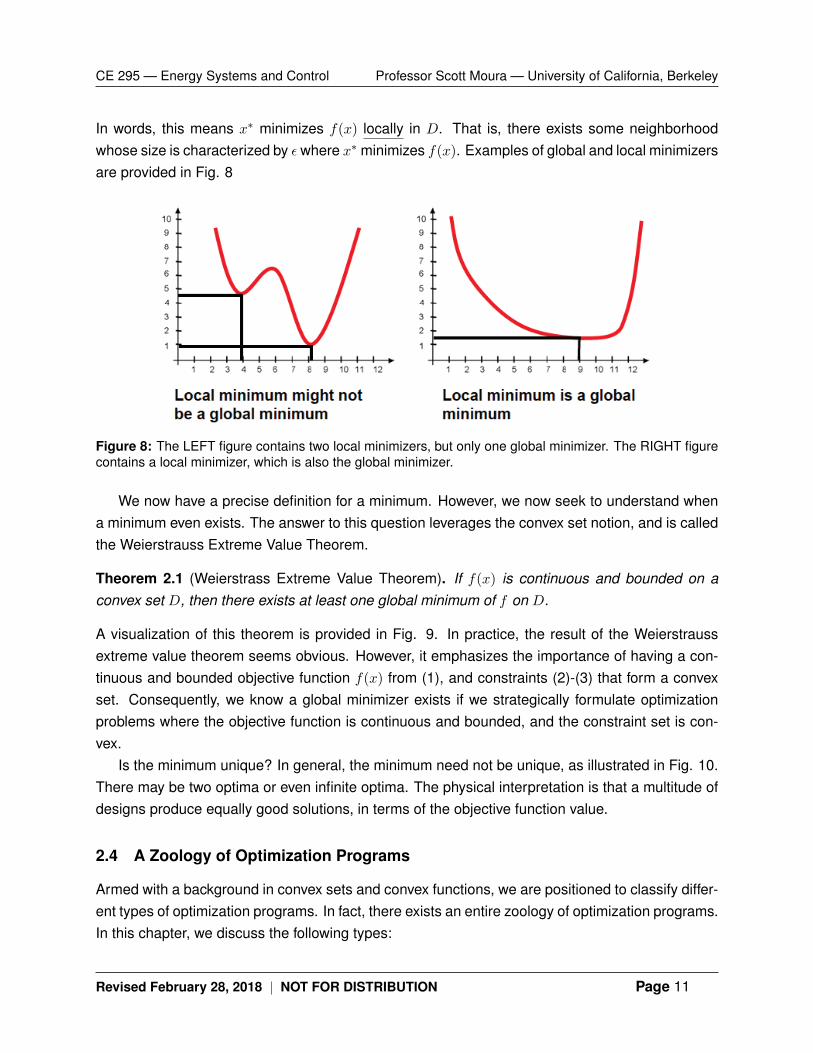
A visualization of this theorem is provided in Fig. 9. In practice, the result of the Weierstraussextreme value theorem seems obvious. However, it emphasizes the importance of having a con-tinuous and bounded objective function f(x) from (1), and constraints (2)-(3) that form a convexset. Consequently, we know a global minimizer exists if we strategically formulate optimizationproblems where the objective function is continuous and bounded, and the constraint set is con-vex.
Is the minimum unique? In general, the minimum need not be unique, as illustrated in Fig. 10.There may be two optima or even infinite optima. The physical interpretation is that a multitude ofdesigns produce equally good solutions, in terms of the objective function value.
2.4 A Zoology of Optimization Programs
Armed with a background in convex sets and convex functions, we are positioned to classify differ-ent types of optimization programs. In fact, there exists an entire zoology of optimization programs.In this chapter, we discuss the following types:
Revised February 28, 2018 | NOT FOR DISTRIBUTION Page 11
CE 295 — Energy Systems and Control Professor Scott Moura — University of California, Berkeley
Figure 9: In this graph, f(x) is continuous andbounded. The convex set is D = [a, b]. The functionf attains a global minimum at x = d and a globalmaximum at x = c.
Figure 10: A local or global minimum need not beunique.
• Linear program (LP)
• Quadratic program (QP)
• Convex program (CP)
• Nonlinear program (NLP)
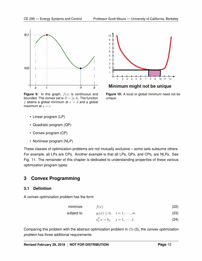
These classes of optimization problems are not mutually exclusive – some sets subsume others.For example, all LPs are CPs. Another example is that all LPs, QPs, and CPs, are NLPs. SeeFig. 11. The remainder of this chapter is dedicated to understanding properties of these variousoptimization program types.
3 Convex Programming
3.1 Definition
A convex optimization problem has the form
minimize f(x) (22)
subject to gi(x) ≤ 0, i = 1, · · · ,m (23)
aTj x = bj , j = 1, · · · , l. (24)
Comparing this problem with the abstract optimization problem in (1)-(3), the convex optimizationproblem has three additional requirements:
Revised February 28, 2018 | NOT FOR DISTRIBUTION Page 12
CE 295 — Energy Systems and Control Professor Scott Moura — University of California, Berkeley
LPQP
CPNLPMIP
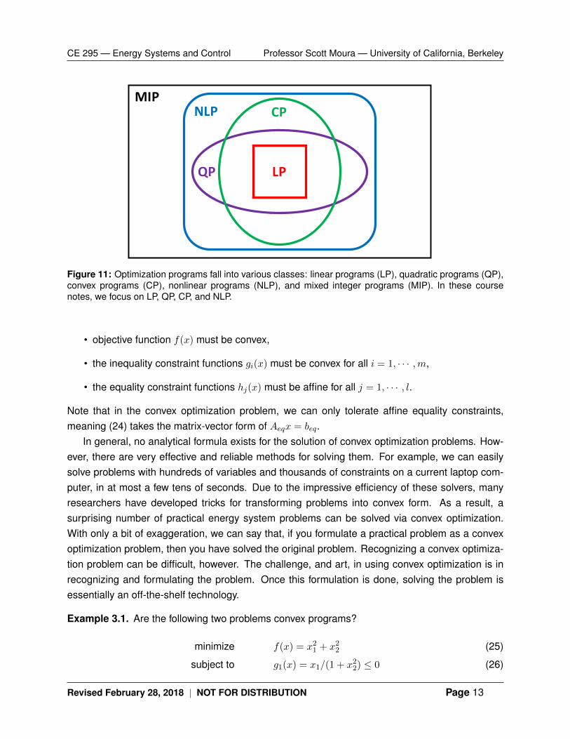
Figure 11: Optimization programs fall into various classes: linear programs (LP), quadratic programs (QP),convex programs (CP), nonlinear programs (NLP), and mixed integer programs (MIP). In these coursenotes, we focus on LP, QP, CP, and NLP.
• objective function f(x) must be convex,
• the inequality constraint functions gi(x) must be convex for all i = 1, · · · ,m,
• the equality constraint functions hj(x) must be affine for all j = 1, · · · , l.
Note that in the convex optimization problem, we can only tolerate affine equality constraints,meaning (24) takes the matrix-vector form of Aeqx = beq.
In general, no analytical formula exists for the solution of convex optimization problems. How-ever, there are very effective and reliable methods for solving them. For example, we can easilysolve problems with hundreds of variables and thousands of constraints on a current laptop com-puter, in at most a few tens of seconds. Due to the impressive efficiency of these solvers, manyresearchers have developed tricks for transforming problems into convex form. As a result, asurprising number of practical energy system problems can be solved via convex optimization.With only a bit of exaggeration, we can say that, if you formulate a practical problem as a convexoptimization problem, then you have solved the original problem. Recognizing a convex optimiza-tion problem can be difficult, however. The challenge, and art, in using convex optimization is inrecognizing and formulating the problem. Once this formulation is done, solving the problem isessentially an off-the-shelf technology.
Example 3.1. Are the following two problems convex programs?
minimize f(x) = x21 + x22 (25)
subject to g1(x) = x1/(1 + x22) ≤ 0 (26)
Revised February 28, 2018 | NOT FOR DISTRIBUTION Page 13
CE 295 — Energy Systems and Control Professor Scott Moura — University of California, Berkeley
h1(x) = (x1 + x2)2 = 0 (27)
This is NOT a convex program. The inequality constraint function g1(x) is not convex in (x1, x2).Additionally, the equality constraint function h1(x) is not affine in (x1, x2).
Now, an astute observer might comment that both sides of (26) can be multiplied by (1 + x22)
and (27) can be represented simply by x1 + x2 = 0, without loss of generality. This leads to:
minimize f(x) = x21 + x22 (28)
subject to g1(x) = x1 ≤ 0 (29)
h1(x) = x1 + x2 = 0 (30)
This is a convex program. The objective function f(x) and inequality constraint function g1(x) areconvex in (x1, x2). Additionally, the equality constraint function h1(x) is affine in (x1, x2).
The remainder of this chapter is dedicated to examples. First, let us discuss some propertiesof convex programs.
3.2 Properties
The following statements are true about convex programming problems:
• If a local minimum exists, then it is the global minimum.
• If the objective function is strictly convex, and a local minimum exists, then it is a uniqueminimum.
The implication of these properties is stunning. The first property states that you need only find alocal minimum (if it exists). In other words, if you can prove that a candidate solution x is optimalover a local neighborhood around x, then you are done. There is no need to search elsewhere.That local optimizer x? is globally optimal.
The second property is also important. If in addition to finding a local minimum, you observethat the objective function is strictly convex (that is, it satisfies (14) with a strict inequality), then thatlocal minimum is unique. That means there exists no other local minimizer x? that does equallywell. You have found the one and only optimal solution.
Next we present a series of important types of convex programs. These examples persistentlyarise in energy systems optimization, along with applications ranging from transportation, environ-mental science & engineering, computer science, structural design, etc. The important examplesinclude:
• Linear programming (LP)
• Quadratic programming (QP)
Revised February 28, 2018 | NOT FOR DISTRIBUTION Page 14
CE 295 — Energy Systems and Control Professor Scott Moura — University of California, Berkeley
• Geometric programming (GP)
• Second order cone programming (SOCP)
• Maximum likelihood estimation (MLE)
3.3 Linear Programming
A linear program (LP) is defined as the following special case of a convex program:
minimize cTx (31)
subject to Ax ≤ b (32)
Aeqx = beq (33)
Compare with the canonical form (1)-(3). We find that f(x) must be linear (or affine, before drop-ping the additive constant). Also, gi(x) and hj(x) must be affine for all i and j, respectively.
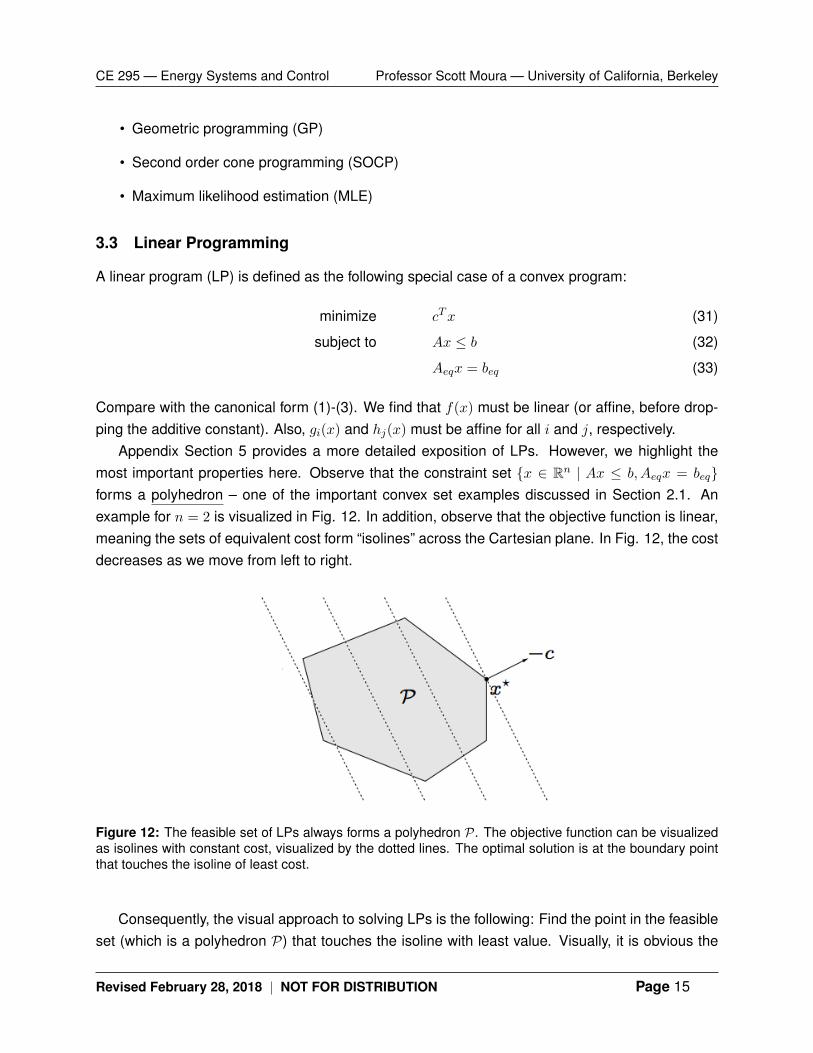
Appendix Section 5 provides a more detailed exposition of LPs. However, we highlight themost important properties here. Observe that the constraint set {x ∈ Rn | Ax ≤ b, Aeqx = beq}forms a polyhedron – one of the important convex set examples discussed in Section 2.1. Anexample for n = 2 is visualized in Fig. 12. In addition, observe that the objective function is linear,meaning the sets of equivalent cost form “isolines” across the Cartesian plane. In Fig. 12, the costdecreases as we move from left to right.
Figure 12: The feasible set of LPs always forms a polyhedron P. The objective function can be visualizedas isolines with constant cost, visualized by the dotted lines. The optimal solution is at the boundary pointthat touches the isoline of least cost.
Consequently, the visual approach to solving LPs is the following: Find the point in the feasibleset (which is a polyhedron P) that touches the isoline with least value. Visually, it is obvious the
Revised February 28, 2018 | NOT FOR DISTRIBUTION Page 15
CE 295 — Energy Systems and Control Professor Scott Moura — University of California, Berkeley
optimum must be bounded (if it is feasible). In other words, the minimizer x? always exists on theboundary of the polyhedron (if it is feasible). This observation leads to the following proposition,provided without proof.
Proposition 2 (LP Solutions). The solution to any linear program is characterized by one of thefollowing three categories:
• [No Solution] This occurs when the feasible set is empty, or the objective function is un-bounded.
• [One Unique Solution] There exists a single unique solution at the vertex of the feasible set.That is, at least two constraints are active and their intersection gives the optimal solution.
• [A Non-Unique Solution] There exists an infinite number of solutions, given by one edgeof the feasible set. That is, one or more constraints are active and all solutions along theintersection of these constraints are equally optimal. This can only occur when the objectivefunction gradient is orthogonal to one or multiple constraint.
Given this foundation, we now dive into examples of LPs in energy systems optimization.
Example 3.2 (Optimal Economic Dispatch). Imagine you are the California Independent SystemOperator (CAISO). Your role is to schedule power plant generation for tomorrow. Specifically, thereare n generators, and you must determine how much power each generator produces during eachone hour increment, across 24 hours. The power generated must equal the power consumed.Moreover, you seek to contract these generators in the most economic fashion possible. Thefollowing data is given:
• Each generator indexed i provides its “marginal cost” ci (units of USD/MW). Quantity ci
indicates the financial compensation each generator requests for providing one unit of power.
• Each generator has a maximum power capacity of xi,max (units of MW). You may not contractmore power than each generator can produce.
• The electricity demand for California isD(k), where k indexes each hour, i.e. k = 0, 1, · · · , 23.
We are now positioned to formulate a LP that can be solved with convex solvers:
minimize23∑k=0
n∑i=1
cixi(k) (34)
subject to 0 ≤ xi(k) ≤ xi,max, ∀ i = 1, · · · , n, k = 0, · · · , 23 (35)n∑i=1
xi(k) = D(k), k = 0, · · · , 23 (36)
Revised February 28, 2018 | NOT FOR DISTRIBUTION Page 16
CE 295 — Energy Systems and Control Professor Scott Moura — University of California, Berkeley
0 6 12 18 240
5
10
15
20
25
30
35
Time of Day
Pow
er
Dem
and [G
W]
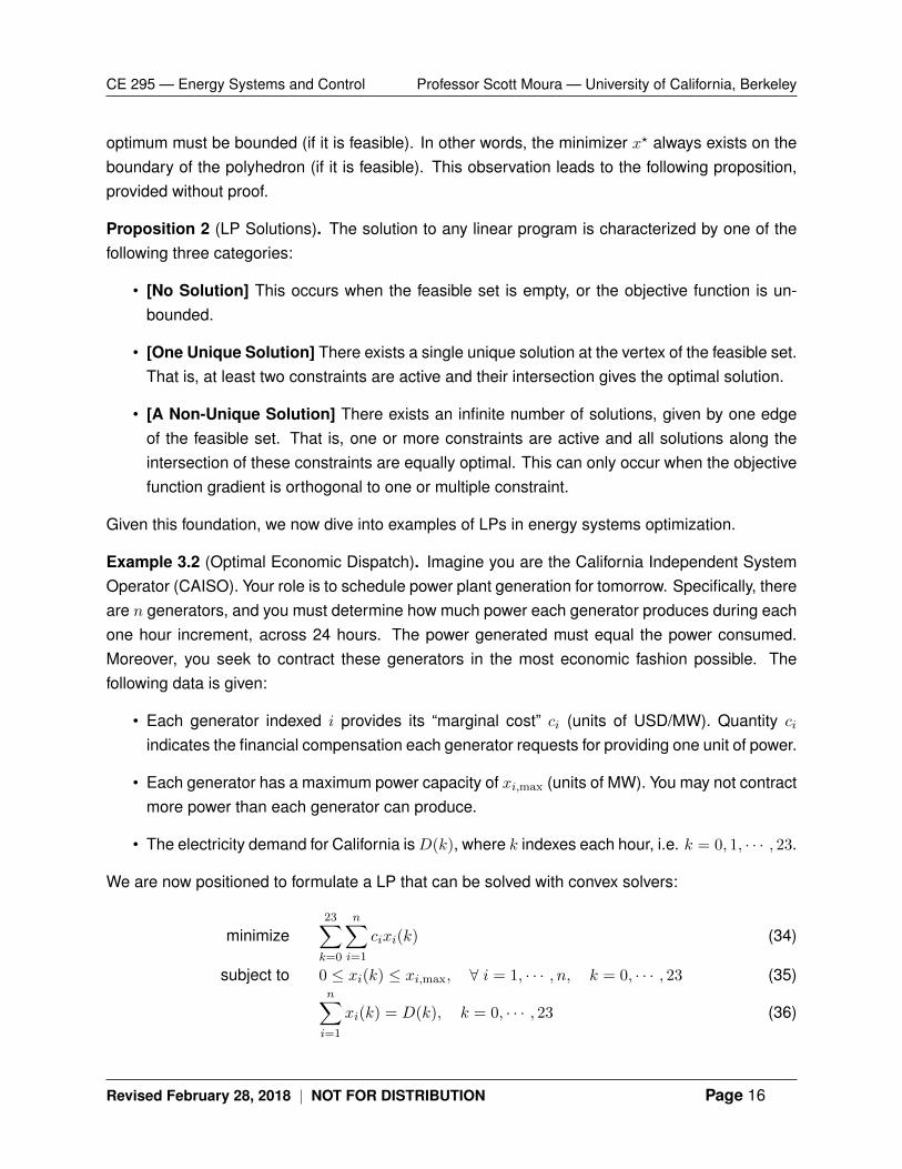
Figure 13: [LEFT] Marginal cost of electricity for various generators, as a function of cumulative capacity.The purple line indicates the total demand D(k). All generators left of the purple line are dispatched.[RIGHT] Optimal supply mix and demand for 03:00.
0 6 12 18 240
5
10
15
20
25
30
35
Time of Day
Pow
er
Dem
and [G
W]
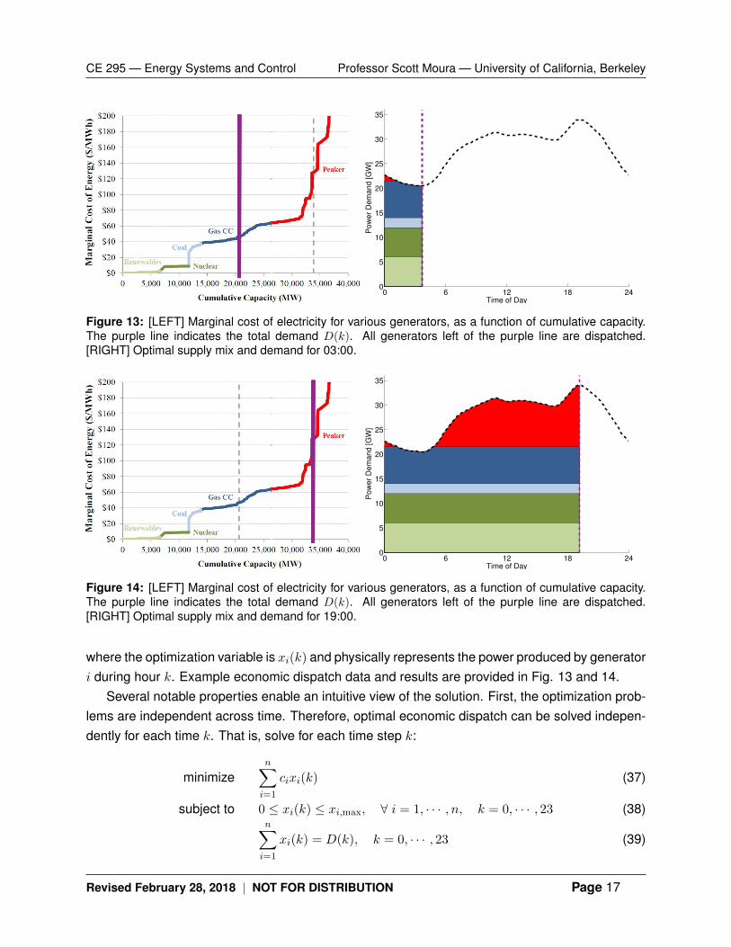
Figure 14: [LEFT] Marginal cost of electricity for various generators, as a function of cumulative capacity.The purple line indicates the total demand D(k). All generators left of the purple line are dispatched.[RIGHT] Optimal supply mix and demand for 19:00.
where the optimization variable is xi(k) and physically represents the power produced by generatori during hour k. Example economic dispatch data and results are provided in Fig. 13 and 14.
Several notable properties enable an intuitive view of the solution. First, the optimization prob-lems are independent across time. Therefore, optimal economic dispatch can be solved indepen-dently for each time k. That is, solve for each time step k:
minimizen∑i=1
cixi(k) (37)
subject to 0 ≤ xi(k) ≤ xi,max, ∀ i = 1, · · · , n, k = 0, · · · , 23 (38)n∑i=1
xi(k) = D(k), k = 0, · · · , 23 (39)
Revised February 28, 2018 | NOT FOR DISTRIBUTION Page 17
CE 295 — Energy Systems and Control Professor Scott Moura — University of California, Berkeley
After solving 24 independent problems, one obtains the minimum generation cost for each hourdenoted f(x?(k)) =
∑ni=1 cix
?i (k). Then the minimum daily generation cost is the sum of minimal
hourly generation costs:∑23
k=0 f(x?(k)).Second, the LP has a specific structure that is often called a “knapsack problem” or a “water-
filling problem”. In this case, we sort the marginal costs in increasing order and compute thecumulative power capacity of the generators. This process yields the [LEFT] plots in Fig. 13 and14. Then we observe the electricity demand, such as 20,000 MW at 03:00 in Fig. 13. In thecumulative capacity vs marginal cost plot, the optimal solution is to dispatch the generators tothe left of the electricity demand. For example, at 03:00 the maximum capacity of renewables,nuclear, and coal is dispatched, and the remaining electricity is delivered by gas combined cycle(CC) plants.
This, of course, is a stylized and simplified version of real-world optimal economic dispatchin power systems. In real power systems, electricity is delivered over a network with variousnetwork constraints. For example, transmission lines and transformers have power limits to ensuresafety. Real-world optimal economic dispatch includes network constraints, that incorporate up tothousands of nodes. This renders a considerably more difficult optimization problem that is almostnever a LP. However, much recent research has focused on clever reformulations into convexprograms.
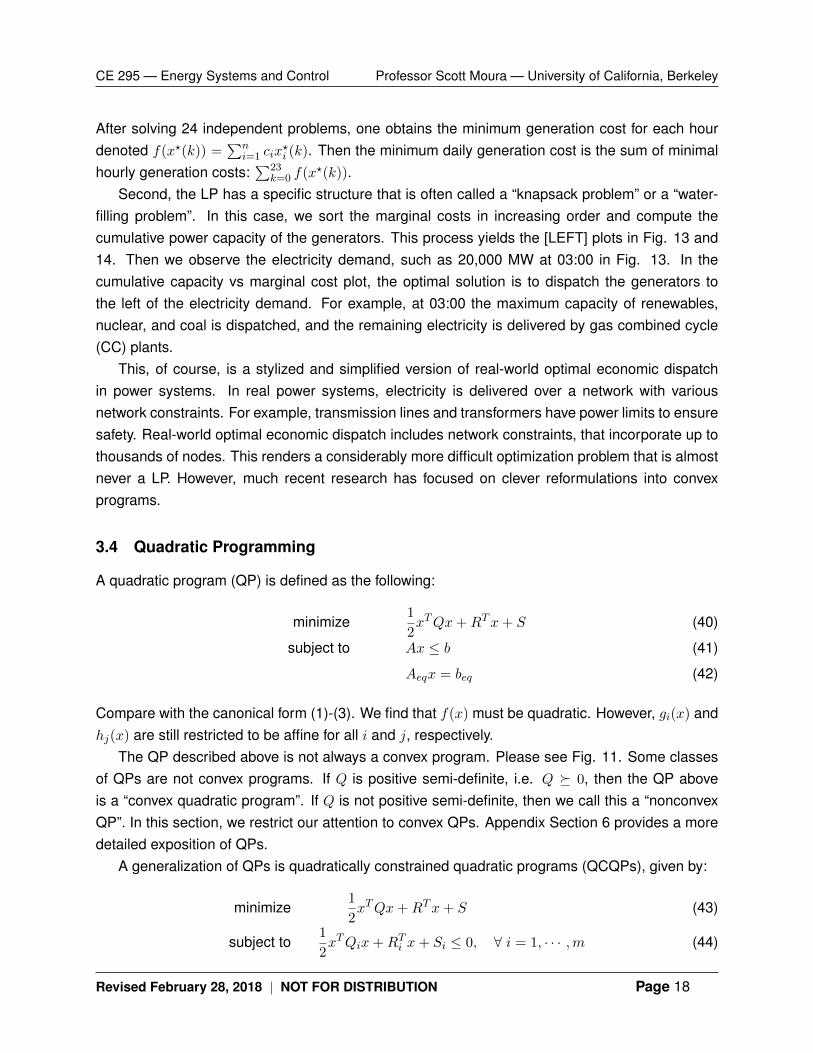
3.4 Quadratic Programming
A quadratic program (QP) is defined as the following:
minimize1
2xTQx+RTx+ S (40)
subject to Ax ≤ b (41)
Aeqx = beq (42)
Compare with the canonical form (1)-(3). We find that f(x) must be quadratic. However, gi(x) andhj(x) are still restricted to be affine for all i and j, respectively.
The QP described above is not always a convex program. Please see Fig. 11. Some classesof QPs are not convex programs. If Q is positive semi-definite, i.e. Q � 0, then the QP aboveis a “convex quadratic program”. If Q is not positive semi-definite, then we call this a “nonconvexQP”. In this section, we restrict our attention to convex QPs. Appendix Section 6 provides a moredetailed exposition of QPs.
A generalization of QPs is quadratically constrained quadratic programs (QCQPs), given by:
minimize1
2xTQx+RTx+ S (43)
subject to1
2xTQix+RTi x+ Si ≤ 0, ∀ i = 1, · · · ,m (44)
Revised February 28, 2018 | NOT FOR DISTRIBUTION Page 18
CE 295 — Energy Systems and Control Professor Scott Moura — University of California, Berkeley
Aeqx = beq (45)
where Q,Qi � 0 for the program to be convex. Compare with the canonical form (1)-(3). We findthat f(x) must be quadratic and now the gi(x) inequality constraint functions may be quadratic forall i. The functions hj(x) must be affine for all j.
Example 3.3 (Markowitz Portfolio Optimization). Imagine you are an investment portfolio manager.You control a large sum of money, which can be invested in up to n assets or stocks. At the endof some time period, your investment produces a financial return. The key challenge, here, is thisreturn is not predictable. It is random.
Denote by xi the fraction of funds invested into asset i. Consequently,∑
i xi = 1 and weassume xi ≥ 0, meaning we cannot invest a negative amount into asset i. (Negative xi is called a“short position”, and implies we are obligated to buy asset i at the end of the investment period.)
Assume the return on each asset can be well-characterized by a multivariate Gaussian distri-bution. Specifically, the return is distributed according to N (µ,Σ), where µ ∈ Rn is the expectedreturn and Σ ∈ Rn×n is the covariance. For example, asset i may have an expected return of µi =
2% with a standard deviation of√
Σii = 5%. In contrast, asset j might have an expected returnof µj = 5%, but a standard deviation of
√Σjj = 50%. Would it be wise to invest everything into
asset j? Would it be wise to invest everything into asset i? What about some mix?This is the classical portfolio optimization problem, introduced by Markowitz. It is mathemati-
cally given as:
minimize xTΣx (46)
subject to µTx ≥ rmin (47)
1Tx = 1, x � 0 (48)
In words, we seek to minimize the return variance while guaranteeing a minimum expected returnof rmin. The final constraint is a budget constraint. This problem is clearly a QP, and can be solvedvia convex solvers. Observe that we are minimizing risk, subject to achieving sufficiently highexpected return. What if we reverse these roles?
Let us consider maximizing expected return, subject to an upper bound on allowed risk. Wewrite:
minimize −µTx (49)
subject to xTΣx ≤ Rmax (50)
1Tx = 1, x � 0 (51)
where Rmax represents the maximum allowable risk. Observe that this problem is a QCQP, whichfollows the form in (43)-(45). This problem can also be solved by convex solvers.
Revised February 28, 2018 | NOT FOR DISTRIBUTION Page 19
CE 295 — Energy Systems and Control Professor Scott Moura — University of California, Berkeley
One common variation is to form a bi-criterion problem. Namely, maximize the expected returnand minimize the return variance. In math:
minimize xTΣx AND maximize µTx (52)
Of course, these two objectives cannot be achieved without tradeoffs. Therefore, one often “scalar-izes” this bi-criterion problem to explore the tradeoff:
minimize −µTx+ γ · xTΣx (53)
subject to 1Tx = 1, x � 0 (54)
where the parameter γ ≥ 0 is called the “risk aversion” parameter. As you increase γ, you becomemore sensitive to variance in your investment returns. A value of γ = 0 classifies you as a purerisk seeker. You ignore variances and simply pursue the highest expected return.
1.02 1.025 1.03 1.035 1.04 1.045 1.05Expected Return [%]
0
0.05
0.1
0.15
0.2
0.25
Ris
k
X: 1.046Y: 0.09999
. = 0
. = 1
Pareto Frontier
. = 0.05
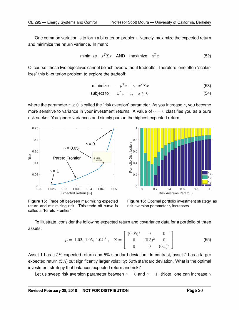
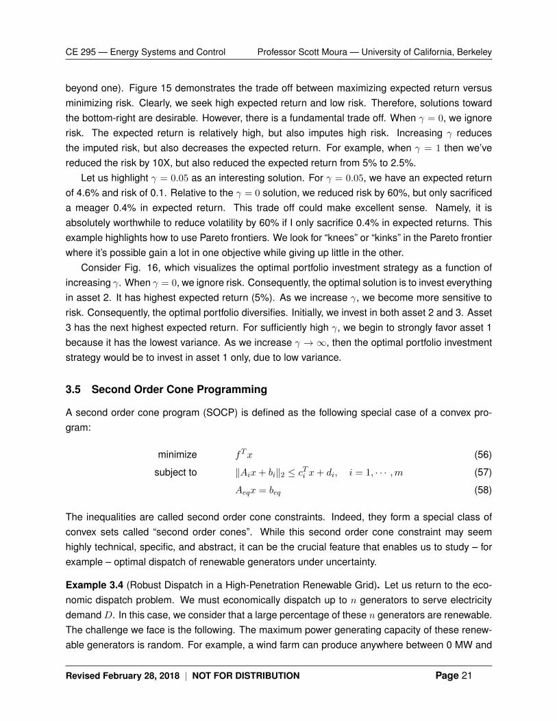
Figure 15: Trade off between maximizing expectedreturn and minimizing risk. This trade off curve iscalled a “Pareto Frontier”
0 0.2 0.4 0.6 0.8 1Risk Aversion Param, .
0
0.2
0.4
0.6
0.8
1P
ortfo
lio D
istr
ibut
ion
x1
x2
x3
Figure 16: Optimal portfolio investment strategy, asrisk aversion parameter γ increases.
To illustrate, consider the following expected return and covariance data for a portfolio of threeassets:
µ = [1.02, 1.05, 1.04]T , Σ =
(0.05)2 0 0
0 (0.5)2 0
0 0 (0.1)2
(55)
Asset 1 has a 2% expected return and 5% standard deviation. In contrast, asset 2 has a largerexpected return (5%) but significantly larger volatility: 50% standard deviation. What is the optimalinvestment strategy that balances expected return and risk?
Let us sweep risk aversion parameter between γ = 0 and γ = 1. (Note: one can increase γ
Revised February 28, 2018 | NOT FOR DISTRIBUTION Page 20
CE 295 — Energy Systems and Control Professor Scott Moura — University of California, Berkeley
beyond one). Figure 15 demonstrates the trade off between maximizing expected return versusminimizing risk. Clearly, we seek high expected return and low risk. Therefore, solutions towardthe bottom-right are desirable. However, there is a fundamental trade off. When γ = 0, we ignorerisk. The expected return is relatively high, but also imputes high risk. Increasing γ reducesthe imputed risk, but also decreases the expected return. For example, when γ = 1 then we’vereduced the risk by 10X, but also reduced the expected return from 5% to 2.5%.
Let us highlight γ = 0.05 as an interesting solution. For γ = 0.05, we have an expected returnof 4.6% and risk of 0.1. Relative to the γ = 0 solution, we reduced risk by 60%, but only sacrificeda meager 0.4% in expected return. This trade off could make excellent sense. Namely, it isabsolutely worthwhile to reduce volatility by 60% if I only sacrifice 0.4% in expected returns. Thisexample highlights how to use Pareto frontiers. We look for “knees” or “kinks” in the Pareto frontierwhere it’s possible gain a lot in one objective while giving up little in the other.
Consider Fig. 16, which visualizes the optimal portfolio investment strategy as a function ofincreasing γ. When γ = 0, we ignore risk. Consequently, the optimal solution is to invest everythingin asset 2. It has highest expected return (5%). As we increase γ, we become more sensitive torisk. Consequently, the optimal portfolio diversifies. Initially, we invest in both asset 2 and 3. Asset3 has the next highest expected return. For sufficiently high γ, we begin to strongly favor asset 1because it has the lowest variance. As we increase γ → ∞, then the optimal portfolio investmentstrategy would be to invest in asset 1 only, due to low variance.
3.5 Second Order Cone Programming
A second order cone program (SOCP) is defined as the following special case of a convex pro-gram:
minimize fTx (56)
subject to ‖Aix+ bi‖2 ≤ cTi x+ di, i = 1, · · · ,m (57)
Aeqx = beq (58)
The inequalities are called second order cone constraints. Indeed, they form a special class ofconvex sets called “second order cones”. While this second order cone constraint may seemhighly technical, specific, and abstract, it can be the crucial feature that enables us to study – forexample – optimal dispatch of renewable generators under uncertainty.
Example 3.4 (Robust Dispatch in a High-Penetration Renewable Grid). Let us return to the eco-nomic dispatch problem. We must economically dispatch up to n generators to serve electricitydemand D. In this case, we consider that a large percentage of these n generators are renewable.The challenge we face is the following. The maximum power generating capacity of these renew-able generators is random. For example, a wind farm can produce anywhere between 0 MW and
Revised February 28, 2018 | NOT FOR DISTRIBUTION Page 21
CE 295 — Energy Systems and Control Professor Scott Moura — University of California, Berkeley
10 MW, depending on weather conditions. Similarly, a solar farm can produce anywhere from 0MW to 20 MW.
To model this scenario, we write the following linear program
minimize fTx (59)
subject to RTx ≥ D (60)
0 ≤ x ≤ 1 (61)
where x ∈ Rn is the vector of power generation dispatched to the generators, as a fraction of thegenerator’s rated capacity. For example, to dispatch 9 MW from the wind farm rated at 10 MW, weset xi = 0.9. To dispatch 15 MW from the solar farm rated at 20 MW, we set xj = 0.75. Parameterf ∈ Rn is the vector of marginal costs, and D ∈ R is the electricity demand. Parameter R ∈ Rn
represents the real-time power capacity of the generators. To convert (59)-(60) into standard form,we define a = −R and b = −D, which yields
minimize fTx (62)
subject to aTx ≤ b (63)
0 ≤ x ≤ 1 (64)
Our primary focus is on parameter a. While parameters f and b are fixed, parameter a isuncertain. In particular, if generator i is the wind farm, then Ri might vary between 0 MW and 10MW (thus −10 ≤ ai ≤ 0). If generator j is the solar farm, then Rj might vary between 0 MW and20 MW (thus −20 ≤ aj ≤ 0). Finally, if generator k is a natural gas plant with 50 MW capacity, thenRk is always 50 MW (thus ak = −50). Mathematically, we hypothesize that vector a is known to liewithin an ellipsoid:
a ∈ E = {a+ Pu | ‖u‖2 ≤ 1} (65)
where a ∈ Rn is the center of this ellipsoid and P ∈ Rn×n is a positive semidefinite matrix. Ifgenerator i is our wind farm with 0 MW to 10 MW capacity, then ai = −5. If generator j is our solarfarm with 0 MW to 20 MW capacity, then aj = −10. If generator k is our conventional natural gasplant with fixed 50 MW capacity, then ak = −50.
Matrix P maps the unit ball ‖u‖2 ≤ 1 into an ellipse. Recall that λ(P ) provides the semi-axislengths. Then we can define P to be a diagonal matrix with its eigenvalues on the diagonal. Forexample, the wind farm with 0 MW to 10 MW capacity would mean Pii = 5. The solar farm with0 MW to 20 MW capacity would mean Pjj = 10. The conventional natural gas plant with fixed 50MW capacity would mean Pkk = 0. In this case, P is positive semi-definite. In a 100% renewablegrid, then P would be strictly positive definite.
Revised February 28, 2018 | NOT FOR DISTRIBUTION Page 22
CE 295 — Energy Systems and Control Professor Scott Moura — University of California, Berkeley
The robust version of (59)-(60) requires us to satisfy demand in EVERY instance of a ∈ E :
minimize fTx (66)
subject to aTx ≤ b, ∀ a ∈ E (67)
0 ≤ x ≤ 1 (68)
Namely, find the optimal economic dispatch which satisfied demand D, given that real-time ca-pacity vector a can exist anywhere in ellipsoid E . An alternative description is the following. Findthe optimal economic dispatch under the worst case scenario of real-time capacity vector a ∈ E .Mathematically, we can reformulate the robust linear constraint (67) to examine the worst case:
max{aTx | a ∈ E
}≤ b (69)
That is, we ensure adequate power generation in the face of uncertain renewable generation byensuring (67) is satisfied in the absolute worst case. We can re-write the left hand side of (69) as
max{aTx | a ∈ E
}= aTx+ max
{uTP Tx | ‖u‖2 ≤ 1
}(70)
= aTx+ ‖P Tx‖2 (71)
Then the robust linear constraint can be re-expressed as
aTx+ ‖P Tx‖2 ≤ b (72)
which is a second order cone constraint. Consequently, a robust LP can be converted to a secondorder cone program (SOCP) – a sub-class of convex optimization problems:
minimize fTx (73)
subject to aTx+ ‖P Tx‖2 ≤ b (74)
0 ≤ x ≤ 1 (75)
Note that the additional norm term acts as a regularization term. Namely, it prevents x frombeing large in directions with considerable uncertainty.
Example 3.5 (Stochastic Dispatch in a High-Penetration Renewable Grid). In the previous exam-ple, we optimize generator dispatch considering the worst-case scenario. One might argue this istoo restrictive. That is, instead of ensuring feasibility for all possible real-time renewable generationcapacity, we could potentially allow violations of (60). These are called “chance constraints.” In theeconomic dispatch application, a separate mechanism could be employed to balance electricitysupply and demand, e.g. demand response, ancillary services, energy storage, etc.
Revised February 28, 2018 | NOT FOR DISTRIBUTION Page 23
CE 295 — Energy Systems and Control Professor Scott Moura — University of California, Berkeley
To formalize this approach, recall the LP
minimize cTx (76)
subject to aTx ≤ b (77)
Assume that a ∈ Rn is Gaussian, i.e. a ∼ N (a,Σ). Then aTx is a Gaussian random variable withmean aTx and variance xTΣx. Hence, we can express the probability that aTx ≤ b is satisfied as
Pr(aTx ≤ b) = Φ
(b− aTx‖Σ1/2x‖2
)(78)
where Φ(x) = (1/√
2π)∫ x−∞ e
−y2/2dy is the CDF of N (0, 1). This enables us to relax (77) into
minimize cTx (79)
subject to Pr(aTx ≤ b) ≥ η (80)
The relaxed constraint (80) is called a chance constraint. Think of it as a reliability prescription.Namely, we require that aTx ≤ b with a reliability of η, where η is typically 0.9, 0.95, or 0.99.Interestingly, we can use (78) to convert this stochastic LP into an SOCP as follows.
minimize cTx (81)
subject to aTx+ Φ−1(η)‖Σ1/2x‖2 ≤ b (82)
where Φ−1(·) is the inverse CDF for the Gaussian distribution. Note that we need Φ−1(·) ≥ 0 to bea valid second order cone constraint. This is true if and only if η ≥ 1/2. Conveniently, we alwayswant a reliability of η ≥ 1/2 in practice.
To summarize, we can formulate a relaxed version of the robust LP problem using chanceconstraints. If the random variable a has a Gaussian distribution, then this chance constrainedLP can be successfully re-formulated into a SOCP, which can be efficiently solved with convexprogramming solvers.
3.6 Maximum Likelihood Estimation
Imagine someone provides you with m data points for random variable y. You seek to fit a prob-ability distribution to this data. In energy systems, variable y could represent wind speed, solarinsolation, vehicle speed, building electricity demand, etc.
We consider a probability density function p(y; θ) for random variable y. Vector θ ∈ Rn pa-rameterizes this density. When p(y; θ) is considered as a function of θ for fixed y, then we callthis a “likelihood function”. As we shall see, it is extremely convenient to use the logarithm of this
Revised February 28, 2018 | NOT FOR DISTRIBUTION Page 24
CE 295 — Energy Systems and Control Professor Scott Moura — University of California, Berkeley
function, which we call the “log-likelihood function”, denoted:
l(θ) = log p(y; θ) (83)
Let us return to the problem of fitting a probability distribution to this data. A standard method,called “maximum likelihood estimation (MLE)”, is to estimate θ as
θ = arg maxθ
p(y; θ) = arg maxθl(θ) (84)
for a given data point y. In this example, the optimization variable is θ. Symbol y is problem data.Interestingly, the MLE problem yields convex optimization problems in many common scenarios.Specifically, (84) is a convex optimization problem if l(θ) is concave w.r.t. θ for each value of y.One can optimally add constraints that form a convex set as well.
Example 3.6 (MLE for Linear Models). For concreteness, we consider a linear measurementmodel,
yi = θTφi + vi, i = 1, · · · ,m (85)
where θ ∈ Rn is the vector of parameters to be estimated, yi ∈ R are the measured data points,φi ∈ Rn are the regressors, and vi ∈ R are the measurement errors or noise. Assume that vi areindependent and identically distributed (IID), with density p(·). The likelihood function, given theyi’s, is given by the products of the likelihood given each measurement yi and regressor φi.
p(v; θ) =m∏i=1
p(yi − θTφi) (86)
The log-likelihood function is then
l(θ) = log p(y; θ) =m∑i=1
log p(yi − θTφi) (87)
HINT: Recall the logarithm of a product property: log(ab) = log(a) + log(b). The MLE problem is:
maximizem∑i=1
log p(yi − θTφi) (88)
w.r.t. variable θ. As mentioned before, p(y; θ) is log-concave for several common probability dis-tributions. For example, suppose that vi are Gaussian with zero mean and variance σ2. Thusp(v) = (2πσ2)−1/2 · e−v2/(2σ2). Substituting this expression for p(·) into (87) gives the log-likelihoodfunction
l(x) = −m2
log(2πσ2)− 1
2σ2‖ΦT θ − y‖22 (89)
Revised February 28, 2018 | NOT FOR DISTRIBUTION Page 25
CE 295 — Energy Systems and Control Professor Scott Moura — University of California, Berkeley
where Φ = [φ1, · · · , φm] ∈ Rn×m is a concatenated matrix of regressor vectors. Consequently, wehave shown the MLE problem for a Gaussian distribution is – quite simply – the solution to theleast-squares problem
θ = arg minθ‖ΦT θ − y‖22 (90)
How elegant!
Exercise 6. Derive the MLE optimization formulation for (85) for the following distributions for vi:
1. Laplacian noise distribution: p(v) = 1/(2a) · e−|v|/a
2. Uniform noise distribution: p(v) = 1/(2a) on [−a,+a] and zero elsewhere
Example 3.7 (Logistic Regression).
Example 3.8 (Mechanical Design w/ Geometric Programs).
3.7 Duality
4 Nonlinear Programming (NLP)
Nonlinear programming problems involve objective functions that are nonlinear in the decisionvariable x. LP and QP problems are special cases of NLPs. As such, the particular structure ofLPs and QPs can be exploited for analysis and computation. In this section, we discuss a moregeneral class of nonlinear problems and corresponding tools for analysis and computation.
A nonlinear optimization problem has the form
minx
f(x) (91)
subject to gi(x) ≤ 0, i = 1, · · · ,m (92)
hj(x) = 0, j = 1, · · · , l. (93)
Note the key difference is the objective function and constraints take a general form that is non-linear in x. In this general case, we first discuss algorithms for the unconstrained case. Then weconsider constraints and present general theory on NLPs.
4.1 Gradient Descent
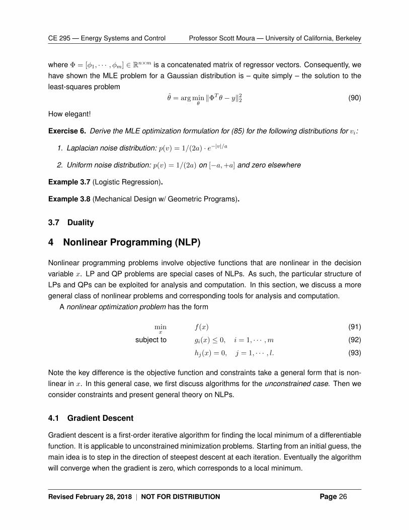
Gradient descent is a first-order iterative algorithm for finding the local minimum of a differentiablefunction. It is applicable to unconstrained minimization problems. Starting from an initial guess, themain idea is to step in the direction of steepest descent at each iteration. Eventually the algorithmwill converge when the gradient is zero, which corresponds to a local minimum.
Revised February 28, 2018 | NOT FOR DISTRIBUTION Page 26
CE 295 — Energy Systems and Control Professor Scott Moura — University of California, Berkeley
This concept is illustrated in Fig. 17, which provides iso-contours of a function f(x) that weseek to minimize. In this example, the user provides an initial guess x0. Then the algorithmproceeds according to
xk+1 = xk − h · ∇f(x) (94)
where h > 0 is some positive step size. The iteration proceeds until a stopping criterion is satisfied.Typically, we stop when the gradient is sufficiently close to zero
‖∇f(xk)‖ ≤ ε (95)
where ε > 0 is some small user defined stopping criterion parameter, and the norm ‖∇f(xk)‖ canbe a user-selected norm, such as the 2-norm, 1-norm, or∞-norm.
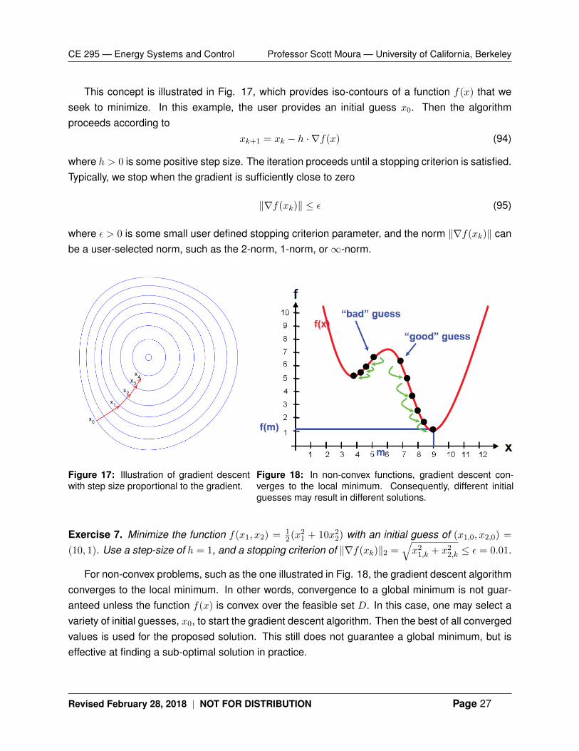
Figure 17: Illustration of gradient descentwith step size proportional to the gradient.
Figure 18: In non-convex functions, gradient descent con-verges to the local minimum. Consequently, different initialguesses may result in different solutions.
Exercise 7. Minimize the function f(x1, x2) = 12(x21 + 10x22) with an initial guess of (x1,0, x2,0) =
(10, 1). Use a step-size of h = 1, and a stopping criterion of ‖∇f(xk)‖2 =√x21,k + x22,k ≤ ε = 0.01.
For non-convex problems, such as the one illustrated in Fig. 18, the gradient descent algorithmconverges to the local minimum. In other words, convergence to a global minimum is not guar-anteed unless the function f(x) is convex over the feasible set D. In this case, one may select avariety of initial guesses, x0, to start the gradient descent algorithm. Then the best of all convergedvalues is used for the proposed solution. This still does not guarantee a global minimum, but iseffective at finding a sub-optimal solution in practice.
Revised February 28, 2018 | NOT FOR DISTRIBUTION Page 27
CE 295 — Energy Systems and Control Professor Scott Moura — University of California, Berkeley
4.2 Barrier and Penalty Functions
A drawback of the gradient descent method is that it does not explicitly account for constraints.Barrier and penalty functions are two methods of augmenting the objective function f(x) to ap-proximately account for the constraints. To illustrate, consider the constrained minimization prob-lem
minx
f(x) (96)
subject to g(x) ≤ 0. (97)
We seek to modify the objective function to account for the constraints, in an approximate way.Thus we can write
minx
f(x) + φ(x; ε) (98)
where φ(x; ε) captures the effect of the constraints and is differentiable, thereby enabling usage ofgradient descent. The parameter ε is a user-defined parameter that allows one to more accuratelyor more coarsely approximate the constraints. Barrier and penalty functions are two methods ofdefining φ(x; ε). The main idea of each is as follows:
• Barrier Function: Allow the objective function to increase towards infinity as x approachesthe constraint boundary from inside the feasible set. In this case, the constraints are guar-anteed to be satisfied, but it is impossible to obtain a boundary optimum.
• Penalty Function: Allow the objective function to increase towards infinity as x violatesthe constraints g(x). In this case, the constraints can be violated, but it allows boundaryoptimum.
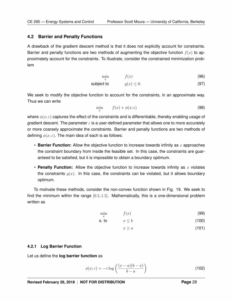
To motivate these methods, consider the non-convex function shown in Fig. 19. We seek tofind the minimum within the range [0.5, 1.5]. Mathematically, this is a one-dimensional problemwritten as
minx
f(x) (99)
s. to x ≤ b (100)
x ≥ a (101)
4.2.1 Log Barrier Function
Let us define the log barrier function as
φ(x; ε) = −ε log
((x− a)(b− x)
b− a
)(102)
Revised February 28, 2018 | NOT FOR DISTRIBUTION Page 28
CE 295 — Energy Systems and Control Professor Scott Moura — University of California, Berkeley
Figure 19: Find the optimum of the function shown above within the range [0.5, 1.5].
The critical property of the log barrier function is that φ(x; ε) → +∞ as x → a from the right sideand x→ b from the left side. Ideally, the log barrier function is zero inside the constraint set. Thisdesired property becomes increasingly true as ε→ 0.
4.2.2 Quadratic Penalty Function
Let us define the quadratic penalty function as
φ(x; ε) =
0 if a ≤ x ≤ b12ε(x− a)2 if x < a
12ε(x− b)
2 if x > b
(103)
The critical property of the quadratic penalty function is that φ(x; ε) increases towards infinity as xincreases beyond b or decreases beyond a. The severity of this increase is parameterized by ε.Also, note that φ(x; ε) is defined such that f(x) + φ(x; ε) remains differentiable at x = a and x = b,thus enabling application of the gradient descent algorithm.
4.3 Sequential Quadratic Programming (SQP)
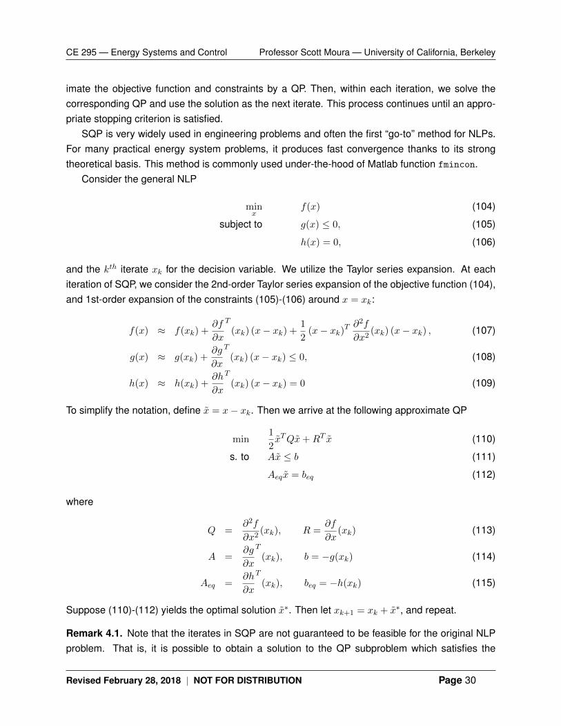
In our discussion of NLPs so far, we have explained how to solve (i) unconstrained problems viagradient method, and (ii) unconstrained problems augmented with barrier or penalty functions toaccount for constraints. In this section, we provide a direct method for handling NLPs with con-straints, called the Sequential Quadratic Programming (SQP) method. The idea is simple. Wesolve a single NLP as a sequence QP subproblems. In particular, at each iteration we approx-
Revised February 28, 2018 | NOT FOR DISTRIBUTION Page 29
CE 295 — Energy Systems and Control Professor Scott Moura — University of California, Berkeley
imate the objective function and constraints by a QP. Then, within each iteration, we solve thecorresponding QP and use the solution as the next iterate. This process continues until an appro-priate stopping criterion is satisfied.
SQP is very widely used in engineering problems and often the first “go-to” method for NLPs.For many practical energy system problems, it produces fast convergence thanks to its strongtheoretical basis. This method is commonly used under-the-hood of Matlab function fmincon.
Consider the general NLP
minx
f(x) (104)
subject to g(x) ≤ 0, (105)
h(x) = 0, (106)
and the kth iterate xk for the decision variable. We utilize the Taylor series expansion. At eachiteration of SQP, we consider the 2nd-order Taylor series expansion of the objective function (104),and 1st-order expansion of the constraints (105)-(106) around x = xk:
f(x) ≈ f(xk) +∂f
∂x
T
(xk) (x− xk) +1
2(x− xk)T
∂2f
∂x2(xk) (x− xk) , (107)
g(x) ≈ g(xk) +∂g
∂x
T
(xk) (x− xk) ≤ 0, (108)
h(x) ≈ h(xk) +∂h
∂x
T
(xk) (x− xk) = 0 (109)
To simplify the notation, define x = x− xk. Then we arrive at the following approximate QP
min1
2xTQx+RT x (110)
s. to Ax ≤ b (111)
Aeqx = beq (112)
where
Q =∂2f
∂x2(xk), R =
∂f
∂x(xk) (113)
A =∂g
∂x
T
(xk), b = −g(xk) (114)
Aeq =∂h
∂x
T
(xk), beq = −h(xk) (115)
Suppose (110)-(112) yields the optimal solution x∗. Then let xk+1 = xk + x∗, and repeat.
Remark 4.1. Note that the iterates in SQP are not guaranteed to be feasible for the original NLPproblem. That is, it is possible to obtain a solution to the QP subproblem which satisfies the
Revised February 28, 2018 | NOT FOR DISTRIBUTION Page 30
CE 295 — Energy Systems and Control Professor Scott Moura — University of California, Berkeley
approximate QP’s constraints, but not the original NLP constraints.
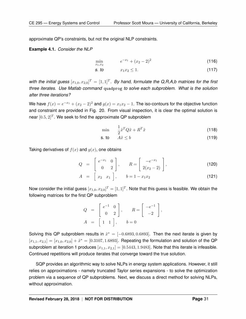
Example 4.1. Consider the NLP
minx1,x2
e−x1 + (x2 − 2)2 (116)
s. to x1x2 ≤ 1. (117)
with the initial guess [x1,0, x2,0]T = [1, 1]T . By hand, formulate the Q,R,A,b matrices for the first
three iterates. Use Matlab command quadprog to solve each subproblem. What is the solutionafter three iterations?
We have f(x) = e−x1 + (x2 − 2)2 and g(x) = x1x2 − 1. The iso-contours for the objective functionand constraint are provided in Fig. 20. From visual inspection, it is clear the optimal solution isnear [0.5, 2]T . We seek to find the approximate QP subproblem
min1
2xTQx+RT x (118)
s. to Ax ≤ b (119)
Taking derivatives of f(x) and g(x), one obtains
Q =
[e−x1 0
0 2
], R =
[−e−x1
2(x2 − 2)
], (120)
A =[x2 x1
], b = 1− x1x2 (121)
Now consider the initial guess [x1,0, x2,0]T = [1, 1]T . Note that this guess is feasible. We obtain the
following matrices for the first QP subproblem
Q =
[e−1 0
0 2
], R =
[−e−1
−2
],
A =[
1 1], b = 0
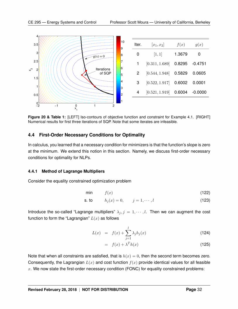
Solving this QP subproblem results in x∗ = [−0.6893, 0.6893]. Then the next iterate is given by[x1,1, x2,1] = [x1,0, x2,0] + x∗ = [0.3107, 1.6893]. Repeating the formulation and solution of the QPsubproblem at iteration 1 produces [x1,1, x2,1] = [0.5443, 1.9483]. Note that this iterate is infeasible.Continued repetitions will produce iterates that converge toward the true solution.
SQP provides an algorithmic way to solve NLPs in energy system applications. However, it stillrelies on approximations - namely truncated Taylor series expansions - to solve the optimizationproblem via a sequence of QP subproblems. Next, we discuss a direct method for solving NLPs,without approximation.
Revised February 28, 2018 | NOT FOR DISTRIBUTION Page 31
CE 295 — Energy Systems and Control Professor Scott Moura — University of California, Berkeley
x1
x2
−2 −1 0 1 20
0.5
1
1.5
2
2.5
3
3.5
4
1
2
3
4
5
6
7
8
9
10
g(x) = 0
Iterations
of SQP
Iter. [x1, x2] f(x) g(x)
0 [1, 1] 1.3679 0
1 [0.311, 1.689] 0.8295 -0.4751
2 [0.544, 1.948] 0.5829 0.0605
3 [0.522, 1.917] 0.6002 0.0001
4 [0.521, 1.919] 0.6004 -0.0000
Figure 20 & Table 1: [LEFT] Iso-contours of objective function and constraint for Example 4.1. [RIGHT]Numerical results for first three iterations of SQP. Note that some iterates are infeasible.
4.4 First-Order Necessary Conditions for Optimality
In calculus, you learned that a necessary condition for minimizers is that the function’s slope is zeroat the minimum. We extend this notion in this section. Namely, we discuss first-order necessaryconditions for optimality for NLPs.
4.4.1 Method of Lagrange Multipliers
Consider the equality constrained optimization problem
min f(x) (122)
s. to hj(x) = 0, j = 1, · · · , l (123)
Introduce the so-called “Lagrange multipliers” λj , j = 1, · · · , l. Then we can augment the costfunction to form the “Lagrangian” L(x) as follows
L(x) = f(x) +
l∑j=1
λjhj(x) (124)
= f(x) + λTh(x) (125)
Note that when all constraints are satisfied, that is h(x) = 0, then the second term becomes zero.Consequently, the Lagrangian L(x) and cost function f(x) provide identical values for all feasiblex. We now state the first-order necessary condition (FONC) for equality constrained problems:
Revised February 28, 2018 | NOT FOR DISTRIBUTION Page 32
CE 295 — Energy Systems and Control Professor Scott Moura — University of California, Berkeley
Proposition 3 (FONC for Equality Constrained NLPs). If a local minimum x∗ exists, then it satisfies
∂L
∂x(x∗) =
∂f
∂x(x∗) + λT
∂h
∂x(x∗) = 0 (stationarity), (126)
∂L
∂λ(x∗) = h(x∗) = 0 (feasibility). (127)
That is, the gradient of the Lagrangian is zero at the minimum x∗.
Remark 4.2. This condition is only necessary. That is, if a local minimum x∗ exists, then it mustsatisfy the FONC. However, a design x which satisfies the FONC isn’t necessarily a local minimum.
Remark 4.3. If the optimization problem is convex, then the FONC is necessary and sufficient.That is, a design x which satisfies the FONC is also a local minimum.
Example 4.2. Consider the equality constrained QP
min1
2xTQx+RTx (128)
s. to Ax = b (129)
Form the Lagrangian,
L(x) =1
2xTQx+RTx+ λT (Ax− b) . (130)
Then the FONC is∂L
∂x(x∗) = Qx∗ +R+ATλ = 0. (131)
Combining the FONC with the equality constraint yields[Q AT
A 0
][x∗
λ
]=
[−Rb
](132)
which provides a set of linear equations that can be solved directly.
Example 4.3. Consider a circle inscribed on a plane, as shown in Fig. 21. Suppose we wish tofind the “lowest” point on the plane while being constrained to the circle. This can be abstractedas the NLP:
min f(x, y) = x+ y (133)
s. to x2 + y2 = 1 (134)
Form the LagrangianL(x, y, λ) = x+ y + λ(x2 + y2 − 1) (135)
Revised February 28, 2018 | NOT FOR DISTRIBUTION Page 33
CE 295 — Energy Systems and Control Professor Scott Moura — University of California, Berkeley
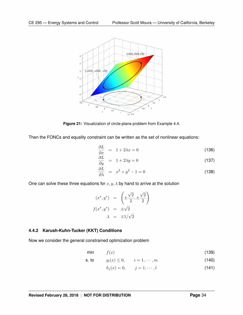
Figure 21: Visualization of circle-plane problem from Example 4.4.
Then the FONCs and equality constraint can be written as the set of nonlinear equations:
∂L
∂x= 1 + 2λx = 0 (136)
∂L
∂y= 1 + 2λy = 0 (137)
∂L
∂λ= x2 + y2 − 1 = 0 (138)
One can solve these three equations for x, y, λ by hand to arrive at the solution
(x∗, y∗) =
(±√
2
2,±√
2
2
)f(x∗, y∗) = ±
√2
λ = ∓1/√
2
4.4.2 Karush-Kuhn-Tucker (KKT) Conditions
Now we consider the general constrained optimization problem
min f(x) (139)
s. to gi(x) ≤ 0, i = 1, · · · ,m (140)
hj(x) = 0, j = 1, · · · , l (141)
Revised February 28, 2018 | NOT FOR DISTRIBUTION Page 34
CE 295 — Energy Systems and Control Professor Scott Moura — University of California, Berkeley
Introduce the so-called “Lagrange multipliers” λj , j = 1, · · · , l each associated with equality con-straints hj(x), j = 1, · · · , l and µi, i = 1, · · · ,m each associated with inequality constraints gi(x), i =
1, · · · ,m. Then we can augment the cost function to form the “Lagrangian” L(x) as follows
L(x) = f(x) +
m∑i=1
µigi(x) +
l∑j=1
λjhj(x) (142)
= f(x) + µT g(x) + λTh(x) (143)
As before, when the equality constraints are satisfied, h(x) = 0, then the third term becomeszero. Elements of the second term become zero in two cases: (i) an inequality constraint is active,that is gi(x) = 0; (ii) the Lagrange multiplier µi = 0. Consequently, the Lagrangian L(x) can beconstructed to have identical values of the cost function f(x) if the aforementioned conditions areapplied. This motivates the first-order necessary conditions (FONC) for the general constrainedoptimization problem – called the Karush-Kuhn-Tucker (KKT) Conditions.
Proposition 4 (KKT Conditions). If x∗ is a local minimum, then the following necessary conditionshold:
∂f
∂x(x∗) +
m∑i=1
µi∂
∂xgi(x
∗) +l∑
j=1
λj∂
∂xhj(x
∗) = 0, Stationarity (144)
gi(x∗) ≤ 0, i = 1, · · · ,m Feasibility (145)
hj(x∗) = 0, j = 1, · · · , l Feasibility (146)
µi ≥ 0, i = 1, · · · ,m Non-negativity (147)
µigi(x∗) = 0, i = 1, · · · ,m Complementary slackness (148)
which can also be written in matrix-vector form as
∂f
∂x(x∗) + µT
∂
∂xg(x∗) + λT
∂
∂xh(x∗) = 0, Stationarity (149)
g(x∗) ≤ 0, Feasibility (150)
h(x∗) = 0, Feasibility (151)
µ ≥ 0, Non-negativity (152)
µT g(x∗) = 0, Complementary slackness (153)
Remark 4.4. Note the following properties of the KKT conditions
• Non-zero µi indicates gi ≤ 0 is active (true with equality). In practice, non-zero µi is how weidentify active constraints from nonlinear solvers.
Revised February 28, 2018 | NOT FOR DISTRIBUTION Page 35
CE 295 — Energy Systems and Control Professor Scott Moura — University of California, Berkeley
• The KKT conditions are necessary, only. That is, if a local minimum x∗ exists, then it mustsatisfy the KKT conditions. However, a design x which satisfies the KKT conditions isn’tnecessarily a local minimum.
• If problem is convex, then the KKT conditions are necessary and sufficient. That is, one maydirectly solve the KKT conditions to obtain the minimum.
• Lagrange multipliers λ, µ are sensitivities to perturbations in the constraints
– In economics, this is called the “shadow price”
– In control theory, this is called the “co-state”
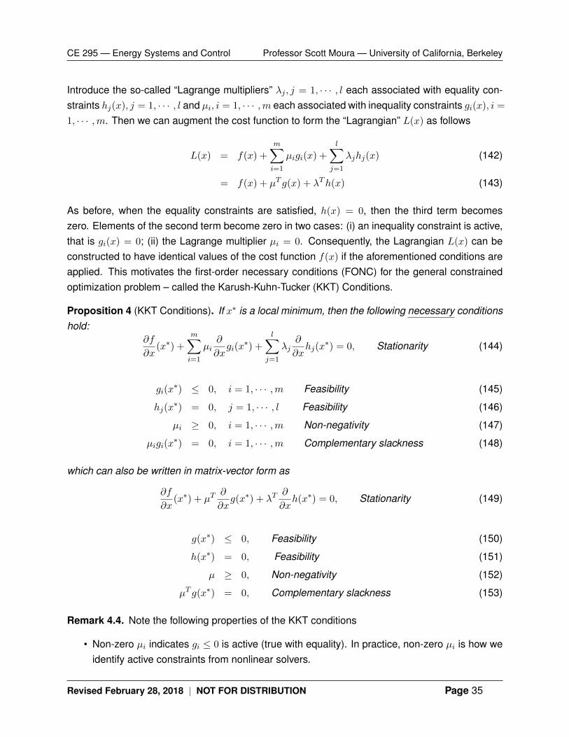
• The KKT conditions have a geometric interpretation demonstrated in Fig. 22. Considerminimizing the cost function with isolines shown in red, where f(x) is increasing as x1, x2increase, as shown by the gradient vector ∇f . Now consider two inequality constraintsg1(x) ≤ 0, g2(x) ≤ 0, forming the feasible set colored in light blue. The gradients at theminimum, weighted by the Lagrange multipliers, are such that their sum equals −∇f . Inother words, the vectors balance to zero according to ∇f(x∗) + µ1∇g1(x∗) + µ2∇g2(x∗) = 0.
µ1∇g1µ2∇g2
g2
g1
x1
x2
∇f Feasible set
isolines
Figure 22: Geometric interpretation of KKT conditions
Example 4.4. Consider again the circle-plane problem, as shown in Fig. 21. Suppose we wish tofind the “lowest” point on the plane while being constrained to within or on the circle. This can beabstracted as the NLP:
min f(x, y) = x+ y (154)
Revised February 28, 2018 | NOT FOR DISTRIBUTION Page 36
CE 295 — Energy Systems and Control Professor Scott Moura — University of California, Berkeley
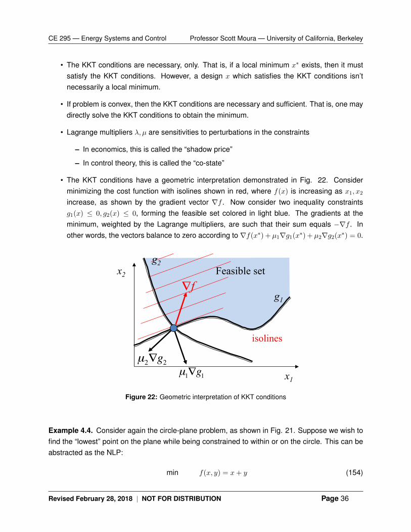
Figure 23: Spring-block system for Example 4.5
s. to x2 + y2 ≤ 1 (155)
Note this problem is convex, therefore the solution to the KKT conditions provides the minimizer(x∗, y∗). We form the Lagrangian
L(x, y, µ) = x+ y + µ(x2 + y2 − 1) (156)
Then the KKT conditions are
∂L
∂x= 1 + 2µx∗ = 0 (157)
∂L
∂y= 1 + 2µy∗ = 0 (158)
∂L
∂µ= (x∗)2 + (y∗)2 − 1 ≤ 0 (159)
µ ≥ 0 (160)
µ((x∗)2 + (y∗)2 − 1
)= 0 (161)
One can solve these equations/inequalities for x∗, y∗, µ by hand to arrive at the solution
(x∗, y∗) =
(−√
2
2,−√
2
2
)f(x∗, y∗) = −
√2
µ = 1/√
2
Example 4.5 (Mechanics Interpretation). Interestingly, the KKT conditions can be used to solvea familiar undergraduate physics example involving the principles of mechanics. Consider twoblocks of width w, where each block is connected to each other and the surrounding walls bysprings, as shown in Fig. 23. Reading left to right, the springs have spring constants k1, k2, k3.The objective is to determine the equilibrium position of the masses. The principles of mechanics
Revised February 28, 2018 | NOT FOR DISTRIBUTION Page 37
CE 295 — Energy Systems and Control Professor Scott Moura — University of California, Berkeley
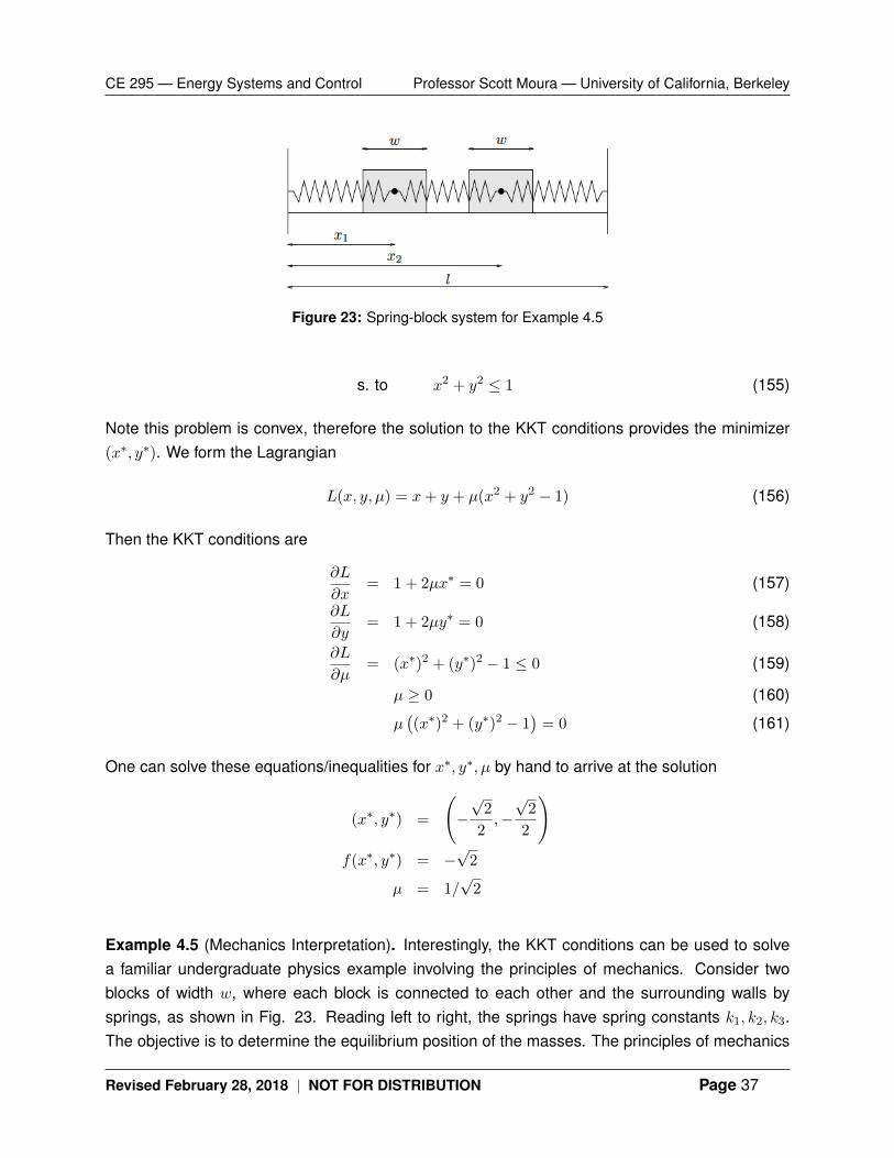
μ1 μ2 μ2 μ3
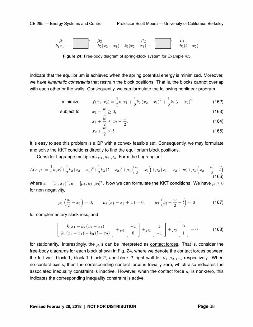
Figure 24: Free-body diagram of spring-block system for Example 4.5
indicate that the equilibrium is achieved when the spring potential energy is minimized. Moreover,we have kinematic constraints that restrain the block positions. That is, the blocks cannot overlapwith each other or the walls. Consequently, we can formulate the following nonlinear program.
minimize f(x1, x2) =1
2k1x
21 +
1
2k2 (x2 − x1)2 +
1
2k3 (l − x2)2 (162)
subject to x1 −w
2≥ 0, (163)
x1 +w
2≤ x2 −
w
2, (164)
x2 +w
2≤ l (165)
It is easy to see this problem is a QP with a convex feasible set. Consequently, we may formulateand solve the KKT conditions directly to find the equilibrium block positions.
Consider Lagrange multipliers µ1, µ2, µ3. Form the Lagrangian:
L(x, µ) =1
2k1x
21+
1
2k2 (x2 − x1)2+
1
2k3 (l − x2)2+µ1
(w2− x1
)+µ2 (x1 − x2 + w)+µ3
(x2 +
w
2− l)
(166)where x = [x1, x2]
T , µ = [µ1, µ2, µ3]T . Now we can formulate the KKT conditions: We have µ ≥ 0
for non-negativity,
µ1
(w2− x1
)= 0, µ2 (x1 − x2 + w) = 0, µ3
(x2 +
w
2− l)
= 0 (167)
for complementary slackness, and[k1x1 − k2 (x2 − x1)
k2 (x2 − x1)− k3 (l − x2)
]+ µ1
[−1
0
]+ µ2
[1
−1
]+ µ3
[0
1
]= 0 (168)
for stationarity. Interestingly, the µi’s can be interpreted as contact forces. That is, consider thefree-body diagrams for each block shown in Fig. 24, where we denote the contact forces betweenthe left wall–block 1, block 1–block 2, and block 2–right wall for µ1, µ2, µ3, respectively. Whenno contact exists, then the corresponding contact force is trivially zero, which also indicates theassociated inequality constraint is inactive. However, when the contact force µi is non-zero, thisindicates the corresponding inequality constraint is active.
Revised February 28, 2018 | NOT FOR DISTRIBUTION Page 38
CE 295 — Energy Systems and Control Professor Scott Moura — University of California, Berkeley
References
[1] P. Denholm, E. Ela, B. Kirby, and M. Milligan, “Role of energy storage with renewable electricity gen-eration,” National Renewable Energy Laboratory (NREL), Golden, CO., Tech. Rep. Technical ReportNREL/TP-6A2-47187, 2010.
[2] “Strategic design of public bicycle sharing systems with service level constraints,” TransportationResearch Part E: Logistics and Transportation Review, vol. 47, no. 2, pp. 284 – 294, 2011.
[3] J. C. Garcia-Palomares, J. Gutierrez, and M. Latorre, “Optimizing the location of stations in bike-sharingprograms: A gis approach,” Applied Geography, vol. 35, no. 1-2, pp. 235–246, 2012.
[4] R. Nair, E. Miller-Hooks, R. C. Hampshire, and A. Busic, “Large-scale vehicle sharing systems: Analysisof velib,” International Journal of Sustainable Transportation, vol. 7, no. 1, pp. 85–106, 2013.
[5] S. Bashash, S. J. Moura, J. C. Forman, and H. K. Fathy, “Plug-in hybrid electric vehicle charge patternoptimization for energy cost and battery longevity,” Journal of Power Sources, vol. 196, no. 1, pp. 541 –549, 2011.
[6] S. J. Tong, A. Same, M. A. Kootstra, and J. W. Park, “Off-grid photovoltaic vehicle charge using secondlife lithium batteries: An experimental and numerical investigation,” Applied Energy, vol. 104, no. 0, pp.740 – 750, 2013.
[7] P. Trnka, J. Pekar, and V. Havlena, “Application of distributed mpc to barcelona water distribution net-work,” in Proceedings of the 18th IFAC World Congress. Milan, Italy, 2011.
[8] S. Boyd and L. Vandenberghe, Convex optimization. Cambridge university press, 2009.
5 Appendix: Linear Programming (LP) in Detail
We begin our exposition of linear programming problems with the following example.
Example 5.1 (Building a Solar Array Farm). You are tasked with designing the parameters of a new photo-voltaic array installation. Namely, you must decide on the square footage of the photovoltaic arrays, and thepower capacity of the power electronics which interface the generators to the grid. The goal is to minimizeinstallation costs, subject to the following constraints:
1. You cannot select negative PV array area, nor negative power electronics power capacity.
2. The minimum generating capacity for the photovoltaic array is gmin.
3. The power capacity of the power electronics must be greater than or equal to the PV array powercapacity.
4. The available spatial area for installation is limited by smax.
5. You have a maximum budget of bmax.
Using the notation in Table 2, we can formulate the following optimization problem:
minx1,x2
c1x1 + c2x2 (169)
Revised February 28, 2018 | NOT FOR DISTRIBUTION Page 39
CE 295 — Energy Systems and Control Professor Scott Moura — University of California, Berkeley
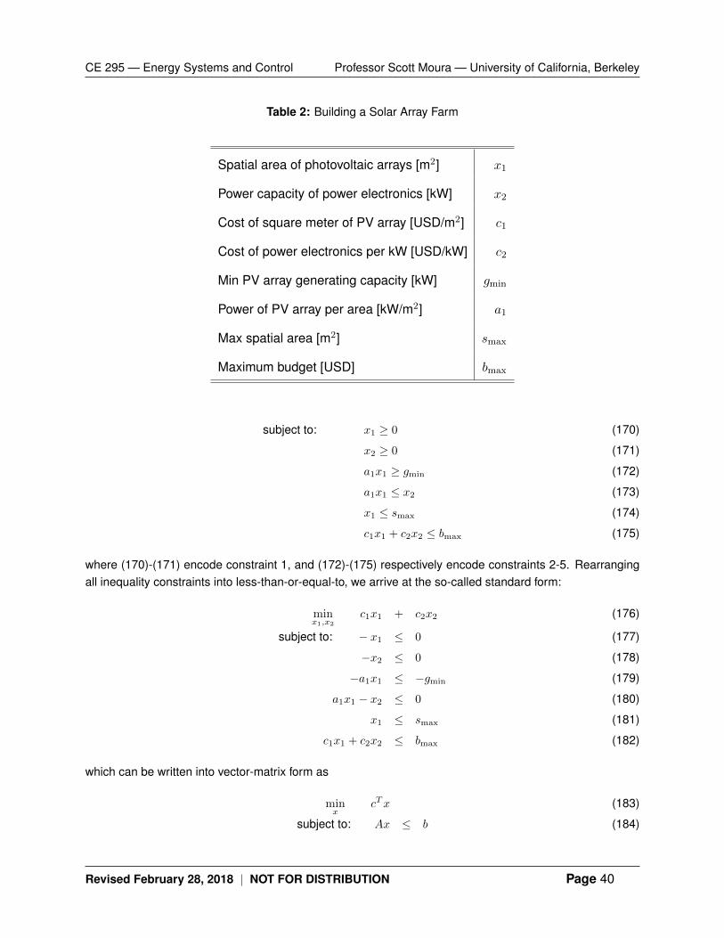
Table 2: Building a Solar Array Farm
Spatial area of photovoltaic arrays [m2] x1
Power capacity of power electronics [kW] x2
Cost of square meter of PV array [USD/m2] c1
Cost of power electronics per kW [USD/kW] c2
Min PV array generating capacity [kW] gmin
Power of PV array per area [kW/m2] a1
Max spatial area [m2] smax
Maximum budget [USD] bmax
subject to: x1 ≥ 0 (170)
x2 ≥ 0 (171)
a1x1 ≥ gmin (172)
a1x1 ≤ x2 (173)
x1 ≤ smax (174)
c1x1 + c2x2 ≤ bmax (175)
where (170)-(171) encode constraint 1, and (172)-(175) respectively encode constraints 2-5. Rearrangingall inequality constraints into less-than-or-equal-to, we arrive at the so-called standard form:
minx1,x2
c1x1 + c2x2 (176)
subject to: − x1 ≤ 0 (177)
−x2 ≤ 0 (178)
−a1x1 ≤ −gmin (179)
a1x1 − x2 ≤ 0 (180)
x1 ≤ smax (181)
c1x1 + c2x2 ≤ bmax (182)
which can be written into vector-matrix form as
minx
cTx (183)
subject to: Ax ≤ b (184)
Revised February 28, 2018 | NOT FOR DISTRIBUTION Page 40
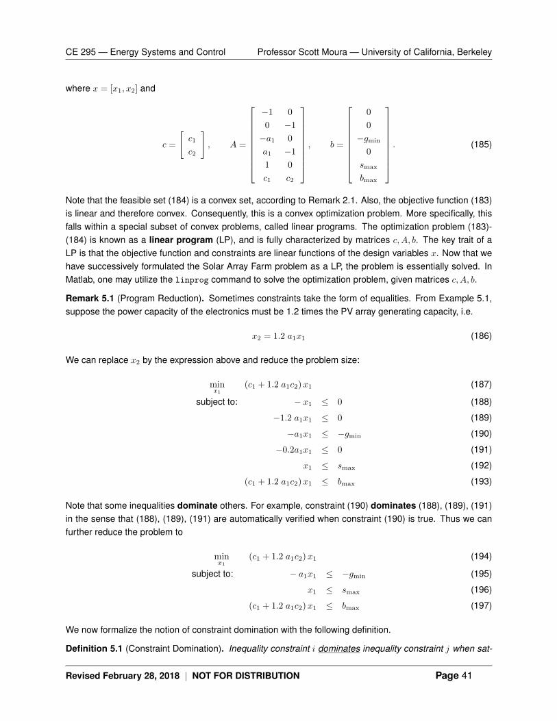
CE 295 — Energy Systems and Control Professor Scott Moura — University of California, Berkeley
where x = [x1, x2] and
c =
[c1
c2
], A =
−1 0
0 −1
−a1 0
a1 −1
1 0
c1 c2
, b =
0
0
−gmin
0
smax
bmax
. (185)
Note that the feasible set (184) is a convex set, according to Remark 2.1. Also, the objective function (183)is linear and therefore convex. Consequently, this is a convex optimization problem. More specifically, thisfalls within a special subset of convex problems, called linear programs. The optimization problem (183)-(184) is known as a linear program (LP), and is fully characterized by matrices c, A, b. The key trait of aLP is that the objective function and constraints are linear functions of the design variables x. Now that wehave successively formulated the Solar Array Farm problem as a LP, the problem is essentially solved. InMatlab, one may utilize the linprog command to solve the optimization problem, given matrices c, A, b.
Remark 5.1 (Program Reduction). Sometimes constraints take the form of equalities. From Example 5.1,suppose the power capacity of the electronics must be 1.2 times the PV array generating capacity, i.e.
x2 = 1.2 a1x1 (186)
We can replace x2 by the expression above and reduce the problem size:
minx1
(c1 + 1.2 a1c2)x1 (187)
subject to: − x1 ≤ 0 (188)
−1.2 a1x1 ≤ 0 (189)
−a1x1 ≤ −gmin (190)
−0.2a1x1 ≤ 0 (191)
x1 ≤ smax (192)
(c1 + 1.2 a1c2)x1 ≤ bmax (193)
Note that some inequalities dominate others. For example, constraint (190) dominates (188), (189), (191)in the sense that (188), (189), (191) are automatically verified when constraint (190) is true. Thus we canfurther reduce the problem to
minx1
(c1 + 1.2 a1c2)x1 (194)
subject to: − a1x1 ≤ −gmin (195)
x1 ≤ smax (196)
(c1 + 1.2 a1c2)x1 ≤ bmax (197)
We now formalize the notion of constraint domination with the following definition.
Definition 5.1 (Constraint Domination). Inequality constraint i dominates inequality constraint j when sat-
Revised February 28, 2018 | NOT FOR DISTRIBUTION Page 41
CE 295 — Energy Systems and Control Professor Scott Moura — University of California, Berkeley
isfaction of constraint j is automatically verified by constraint i.
Continuing with our example, intuition suggests we can minimize costs by selecting the spatial area x1such that the minimum generating capacity is met exactly1. That is, at the optimal solution x∗1, constraint(190) is true with equality. This produces the minimizer x∗1 = gmin/a1 and the minimum installation cost(c1 + 1.2 a1 c2) gmin/a1. Note that we denote minimizers with the star notation: x∗1. Also, when an inequalityconstraint is true with equality at the optimum, we call the constraint an active constraint.
Definition 5.2 (Active Inequalities). Constraint i is called an active constraint when it is true with equality atthe optimum.
5.1 General Form of LP
Linear programs can be identified as having linear objective functions and linear constraints. Suppose wehave N decision variables xi, M inequality constraints, and L equality constraints. Mathematically, thistakes the form
min c1x1 + c2x2 + . . .+ cNxN
subject to: a1,1x1 + a1,2x2 + . . .+ a1,NxN ≤ b1,
a2,1x1 + a2,2x2 + . . .+ a2,NxN ≤ b2,
...
aM,1x1 + aM,2x2 + . . .+ aM,NxN ≤ bM ,
aeq,1,1x1 + aeq,1,2x2 + . . .+ aeq,1,NxN = beq,1,
aeq,2,1x1 + aeq,2,2x2 + . . .+ aeq,2,NxN = beq,2,
...
aeq,L,1x1 + aeq,L,2x2 + . . .+ aeq,L,NxN = beq,L,
We may equivalently write this problem in “Sigma” notation as follows:
min
N∑k=1
ckxk
subject to:N∑
k=1
a1,kxk ≤ b1,
N∑k=1
a2,kxk ≤ b2,
...N∑
k=1
aM,kxk ≤ bM ,
1Naturally, this assumes the problem parameters are such that the feasible set is non-empty, that is, some solutionexists.
Revised February 28, 2018 | NOT FOR DISTRIBUTION Page 42
CE 295 — Energy Systems and Control Professor Scott Moura — University of California, Berkeley
N∑k=1
aeq,1,kxk = beq,1,
N∑k=1
aeq,2,kxk = beq,2,
...N∑
k=1
aeq,L,kxk = beq,L
The most compact notation uses matrix-vector format, and is given by
min cTx
subject to: Ax ≤ b,
Aeqx = beq,
where
x = [x1, x2, . . . , xN ]T
c = [c1, c2, . . . , cN ]T
[A]i,j = ai,j , A ∈ RM×N
b = [b1, b2, . . . , bM ]T, b ∈ RM
[Aeq]i,j = aeq,i,j , Aeq ∈ RL×N
beq = [beq,1, beq,2, . . . , beq,L]T, beq ∈ RL
5.2 Graphical LP
For problems of one, two, or sometimes three dimensions, we can use graphical methods to visualize thefeasible sets and solutions. This visualization provides excellent intuition for the nature of LP solutions. Wedemonstrate with the following example.
max Z = 140x1 + 160x2
s. to 2x1 + 4x2 ≤ 28
5x1 + 5x2 ≤ 50
x1 ≤ 8
x2 ≤ 6
x1 ≥ 0
x2 ≥ 0
On a graph, one may successively plot each of the inequality constraints and divide the Cartesian space intofeasible “half-spaces.” As each half-space is identified, we retain the intersection of the remaining feasible
Revised February 28, 2018 | NOT FOR DISTRIBUTION Page 43
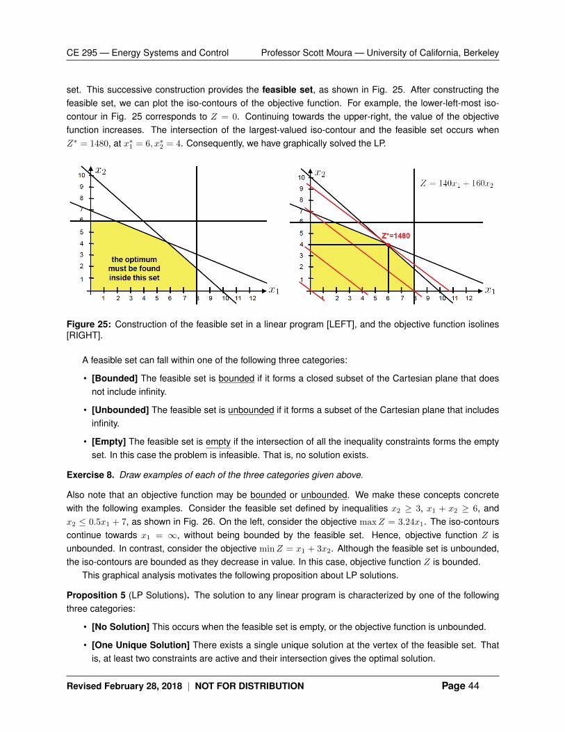
CE 295 — Energy Systems and Control Professor Scott Moura — University of California, Berkeley
set. This successive construction provides the feasible set, as shown in Fig. 25. After constructing thefeasible set, we can plot the iso-contours of the objective function. For example, the lower-left-most iso-contour in Fig. 25 corresponds to Z = 0. Continuing towards the upper-right, the value of the objectivefunction increases. The intersection of the largest-valued iso-contour and the feasible set occurs whenZ∗ = 1480, at x∗1 = 6, x∗2 = 4. Consequently, we have graphically solved the LP.
Figure 25: Construction of the feasible set in a linear program [LEFT], and the objective function isolines[RIGHT].
A feasible set can fall within one of the following three categories:
• [Bounded] The feasible set is bounded if it forms a closed subset of the Cartesian plane that doesnot include infinity.
• [Unbounded] The feasible set is unbounded if it forms a subset of the Cartesian plane that includesinfinity.
• [Empty] The feasible set is empty if the intersection of all the inequality constraints forms the emptyset. In this case the problem is infeasible. That is, no solution exists.
Exercise 8. Draw examples of each of the three categories given above.
Also note that an objective function may be bounded or unbounded. We make these concepts concretewith the following examples. Consider the feasible set defined by inequalities x2 ≥ 3, x1 + x2 ≥ 6, andx2 ≤ 0.5x1 + 7, as shown in Fig. 26. On the left, consider the objective maxZ = 3.24x1. The iso-contourscontinue towards x1 = ∞, without being bounded by the feasible set. Hence, objective function Z isunbounded. In contrast, consider the objective minZ = x1 + 3x2. Although the feasible set is unbounded,the iso-contours are bounded as they decrease in value. In this case, objective function Z is bounded.
This graphical analysis motivates the following proposition about LP solutions.
Proposition 5 (LP Solutions). The solution to any linear program is characterized by one of the followingthree categories:
• [No Solution] This occurs when the feasible set is empty, or the objective function is unbounded.
• [One Unique Solution] There exists a single unique solution at the vertex of the feasible set. Thatis, at least two constraints are active and their intersection gives the optimal solution.
Revised February 28, 2018 | NOT FOR DISTRIBUTION Page 44
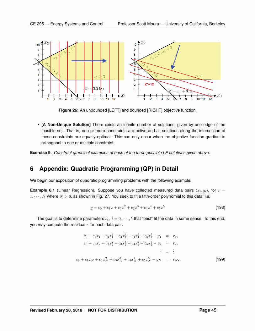
CE 295 — Energy Systems and Control Professor Scott Moura — University of California, Berkeley
Figure 26: An unbounded [LEFT] and bounded [RIGHT] objective function.
• [A Non-Unique Solution] There exists an infinite number of solutions, given by one edge of thefeasible set. That is, one or more constraints are active and all solutions along the intersection ofthese constraints are equally optimal. This can only occur when the objective function gradient isorthogonal to one or multiple constraint.
Exercise 9. Construct graphical examples of each of the three possible LP solutions given above.
6 Appendix: Quadratic Programming (QP) in Detail
We begin our exposition of quadratic programming problems with the following example.
Example 6.1 (Linear Regression). Suppose you have collected measured data pairs (xi, yi), for i =
1, · · · , N where N > 6, as shown in Fig. 27. You seek to fit a fifth-order polynomial to this data, i.e.
y = c0 + c1x+ c2x2 + c3x
3 + c4x4 + c5x
5 (198)
The goal is to determine parameters ci, i = 0, · · · , 5 that “best” fit the data in some sense. To this end,you may compute the residual r for each data pair:
c0 + c1x1 + c2x21 + c3x
31 + c4x
41 + c5x
51 − y1 = r1,
c0 + c1x2 + c2x22 + c3x
32 + c4x
42 + c5x
52 − y2 = r2,
... =...
c0 + c1xN + c2x2N + c3x
3N + c4x
4N + c5x
5N − yN = rN , (199)
Revised February 28, 2018 | NOT FOR DISTRIBUTION Page 45
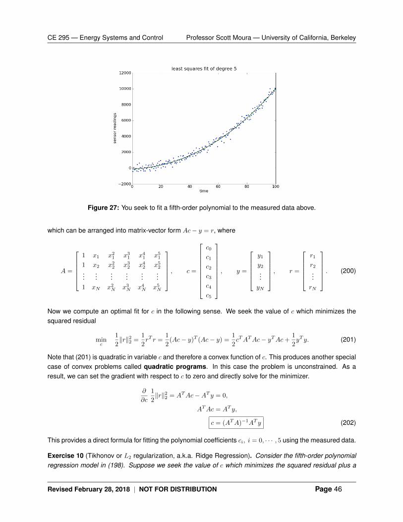
CE 295 — Energy Systems and Control Professor Scott Moura — University of California, Berkeley
Figure 27: You seek to fit a fifth-order polynomial to the measured data above.
which can be arranged into matrix-vector form Ac− y = r, where
A =
1 x1 x21 x31 x41 x511 x2 x22 x32 x42 x52...
......
......
...1 xN x2N x3N x4N x5N
, c =
c0
c1
c2
c3
c4
c5
, y =
y1
y2...yN
, r =
r1
r2...rN
. (200)
Now we compute an optimal fit for c in the following sense. We seek the value of c which minimizes thesquared residual
minc
1
2‖r‖22 =
1
2rT r =
1
2(Ac− y)T (Ac− y) =
1
2cTATAc− yTAc+
1
2yT y. (201)
Note that (201) is quadratic in variable c and therefore a convex function of c. This produces another specialcase of convex problems called quadratic programs. In this case the problem is unconstrained. As aresult, we can set the gradient with respect to c to zero and directly solve for the minimizer.
∂
∂c
1
2‖r‖22 = ATAc−AT y = 0,
ATAc = AT y,
c = (ATA)−1AT y (202)
This provides a direct formula for fitting the polynomial coefficients ci, i = 0, · · · , 5 using the measured data.
Exercise 10 (Tikhonov or L2 regularization, a.k.a. Ridge Regression). Consider the fifth-order polynomialregression model in (198). Suppose we seek the value of c which minimizes the squared residual plus a
Revised February 28, 2018 | NOT FOR DISTRIBUTION Page 46
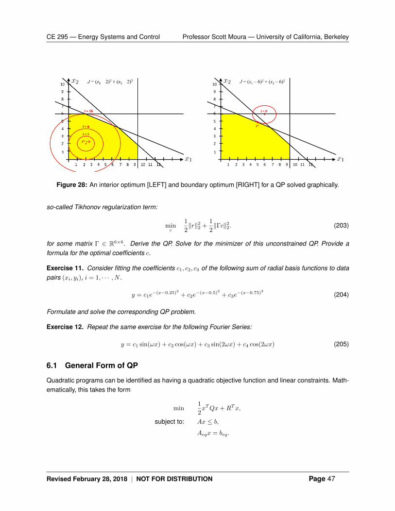
CE 295 — Energy Systems and Control Professor Scott Moura — University of California, Berkeley
1
9
1 2 3 4 5 6 7 8 9 10 11 12
1
2
3
4
5
6 7
8
9
10 J = (x1 – 6)2 + (x2 – 6)2
J = 0
J*
Figure 28: An interior optimum [LEFT] and boundary optimum [RIGHT] for a QP solved graphically.
so-called Tikhonov regularization term:
minc
1
2‖r‖22 +
1
2‖Γc‖22. (203)
for some matrix Γ ∈ R6×6. Derive the QP. Solve for the minimizer of this unconstrained QP. Provide aformula for the optimal coefficients c.
Exercise 11. Consider fitting the coefficients c1, c2, c3 of the following sum of radial basis functions to datapairs (xi, yi), i = 1, · · · , N .
y = c1e−(x−0.25)2 + c2e
−(x−0.5)2 + c3e−(x−0.75)2 (204)
Formulate and solve the corresponding QP problem.
Exercise 12. Repeat the same exercise for the following Fourier Series:
y = c1 sin(ωx) + c2 cos(ωx) + c3 sin(2ωx) + c4 cos(2ωx) (205)
6.1 General Form of QP
Quadratic programs can be identified as having a quadratic objective function and linear constraints. Math-ematically, this takes the form
min1
2xTQx+RTx,
subject to: Ax ≤ b,
Aeqx = beq.
Revised February 28, 2018 | NOT FOR DISTRIBUTION Page 47
CE 295 — Energy Systems and Control Professor Scott Moura — University of California, Berkeley
6.2 Graphical QP
For problems of one, two, or three dimensions, it is possible to solve QPs graphically. Consider the followingQP example:
min J = (x1 − 2)2 + (x2 − 2)2
s. to 2x1 + 4x2 ≤ 28
5x1 + 5x2 ≤ 50
x1 ≤ 8
x2 ≤ 6
x1 ≥ 0
x2 ≥ 0
The feasible set and corresponding iso-contours are illustrated in the left-hand side of Fig. 28. In this case,the solution is an interior optimum. That is, no constraints are active at the minimum. In contrast, considerthe objective function J = (x1 − 6)2 + (x2 − 6)2 shown on the right-hand side of Fig. 28. In this case, theminimum occurs at the boundary and is unique.
Revised February 28, 2018 | NOT FOR DISTRIBUTION Page 48