Embed Size (px)
Citation preview

1
Music Classification Using SVM
Ming-jen Wang
Chia-Jiu Wang
2
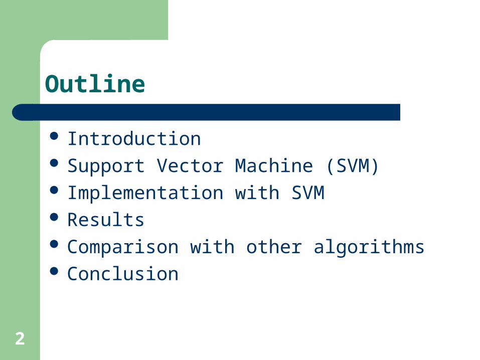
Outline
Introduction Support Vector Machine (SVM) Implementation with SVM Results Comparison with other algorithms Conclusion

3
Music Genre Classification
Human can identify music genre easily.
(play clips)
How could machines perform this task?
What would make it easier for machines?
What are the differences between the genres?
4
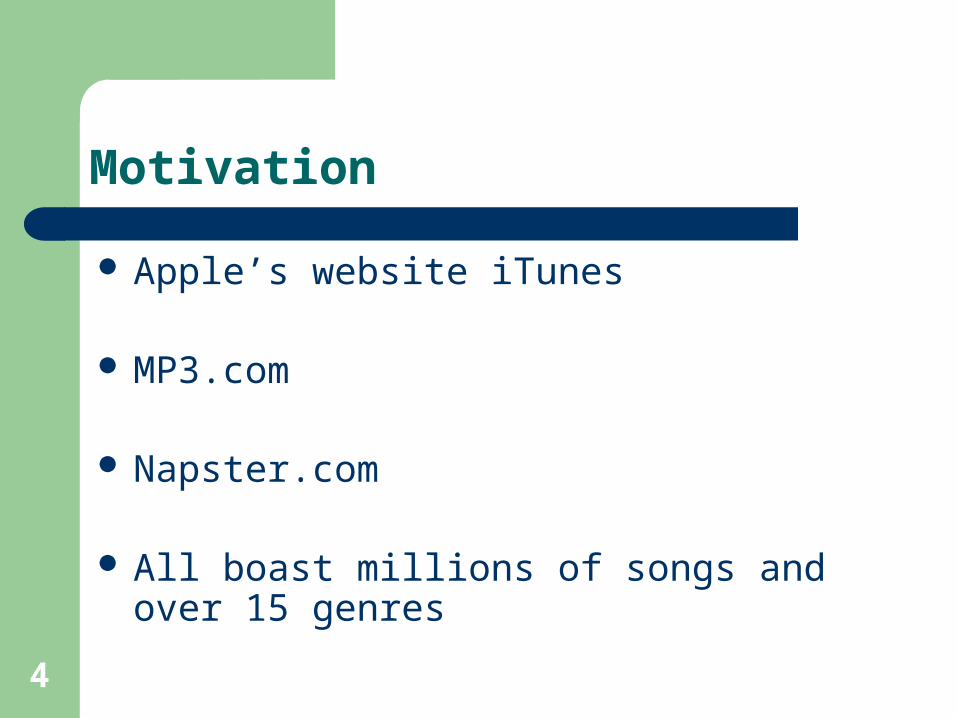
Motivation
Apple’s website iTunes
MP3.com
Napster.com
All boast millions of songs and over 15 genres
5
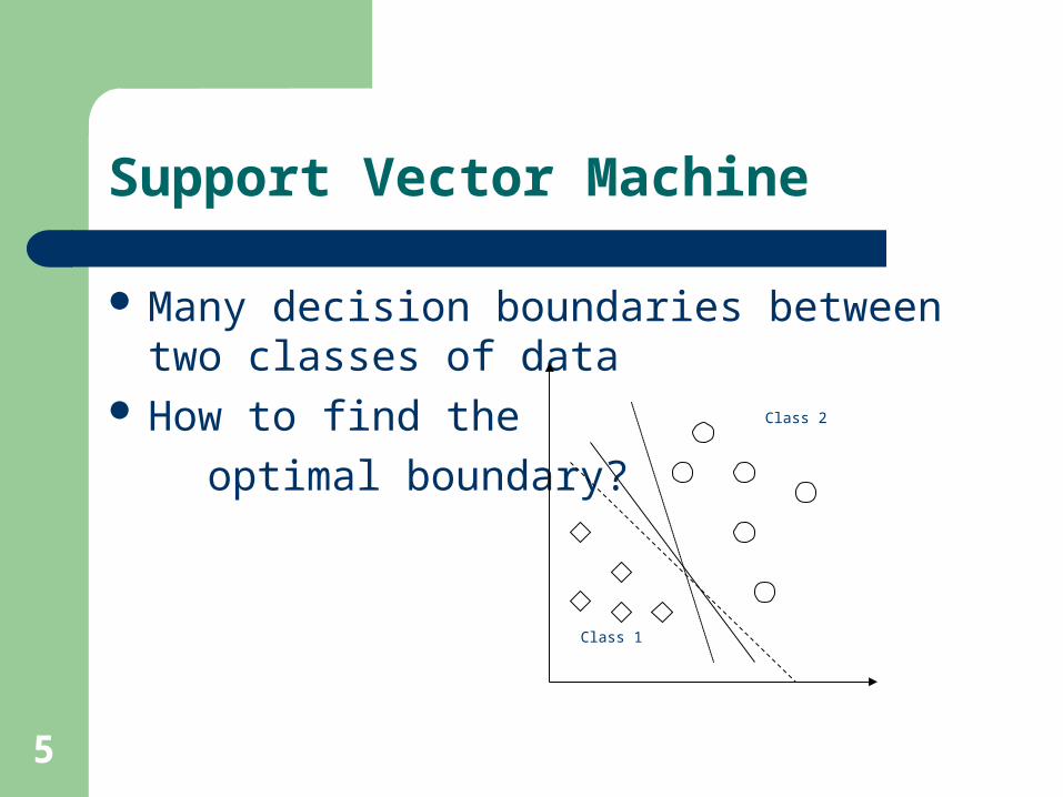
Support Vector Machine
Many decision boundaries between two classes of data
How to find the
optimal boundary?
Class 2
Class 1

6
Support Vectors
Linear SVMClass 2
Class 1
m
wTxi+b = -1
wTxi+b = 0
wTxi+b = 1
x-
x+
0)( bxwxg iT
i
}1)(|1{ ii xgy
}1)(|1{ ii xgy
7
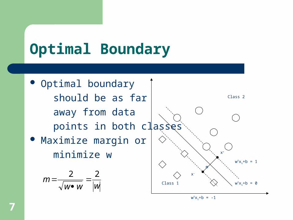
Optimal Boundary
Optimal boundary
should be as far
away from data
points in both classes Maximize margin or
minimize w
Class 2
Class 1
m
wTxi+b = -1
wTxi+b = 0
wTxi+b = 1
x-
x+
wwwm
22
8
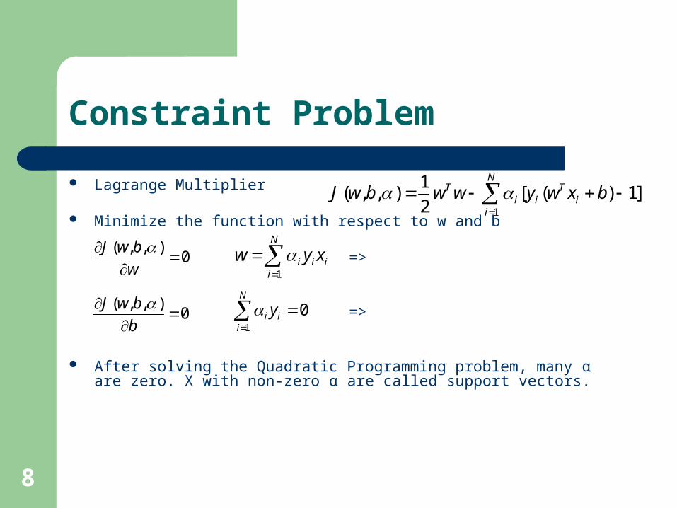
Constraint Problem
Lagrange Multiplier
Minimize the function with respect to w and b
=>
=>
After solving the Quadratic Programming problem, many α are zero. X with non-zero α are called support vectors.
N
ii
Tii
T bxwywwbwJ1
]1)([2
1),,(
0),,(
w
bwJ
0),,(
b
bwJ
N
iiii xyw
1
N
iii y
1
0
9
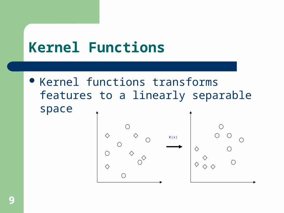
Kernel Functions
Kernel functions transforms features to a linearly separable space
K(x)
10
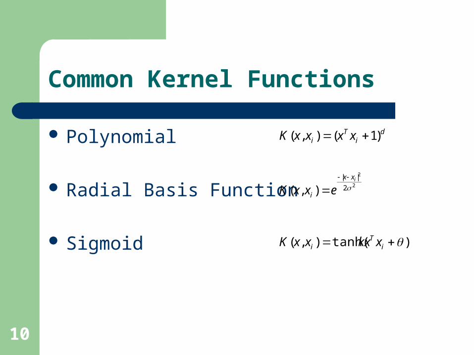
Common Kernel Functions
Polynomial
Radial Basis Function
Sigmoid
di
Ti xxxxK )1(),(
2
2
2
||
),( ixx
i exxK
)tanh(),( iT
i xkxxxK
11
Implementation
Quadratic Programming
MySVM by Stefan Rueping
Matlab scripts

12
Example
Training data points
0 2 4 6 8 10 05
10
0
5
10
15
20
25
13
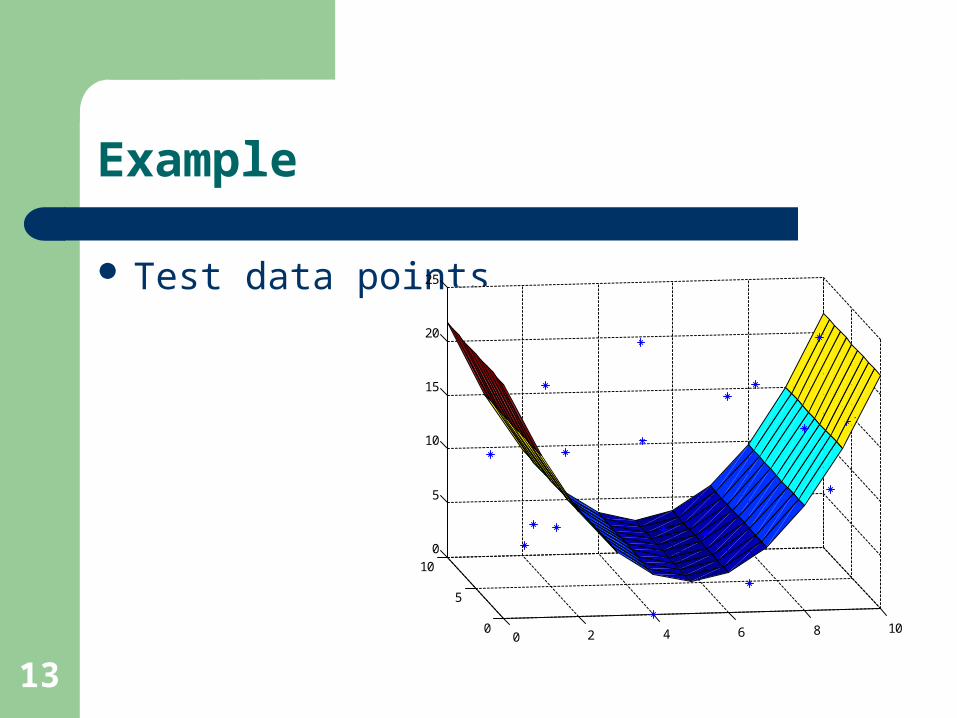
Example
Test data points
0 2 4 6 8 100
5
100
5
10
15
20
25

14
Example
@examples # svm example set dimension 3 number 20 b 2.25393 format xy 1 3 5 -2.51502 2 4 6 -0.420652 1 9 10 -2.17461 10 5 15 -0.824929 7 3 1 -2.51759 9 2 10 -0.835865 2 8 4 -2.24897
10 6 14 -1.35431 4 0 0 -4.10939 8 8 2 -3.44793 5 5 5 0.917108 3 9 10 1.4258 4 2 15 2.70503 7 2 20 4.81161 8 0 17 2.36853 9 4 23 5.4079 2 6 18 0.822491 6 4 5 0.585008 7 7 16 2.44882 5 9 20 2.64036

15
Classifying Music Genres
Many features to choose from
Using FFT spectrum
Classical, Jazz and Rock
Each genre has its dynamic range
16
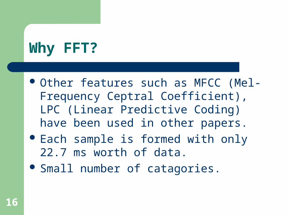
Why FFT?
Other features such as MFCC (Mel-Frequency Ceptral Coefficient), LPC (Linear Predictive Coding) have been used in other papers.
Each sample is formed with only 22.7 ms worth of data.
Small number of catagories.
17
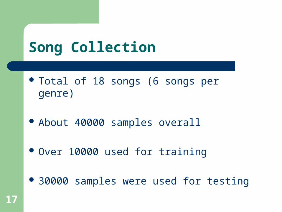
Song Collection
Total of 18 songs (6 songs per genre)
About 40000 samples overall
Over 10000 used for training
30000 samples were used for testing
18
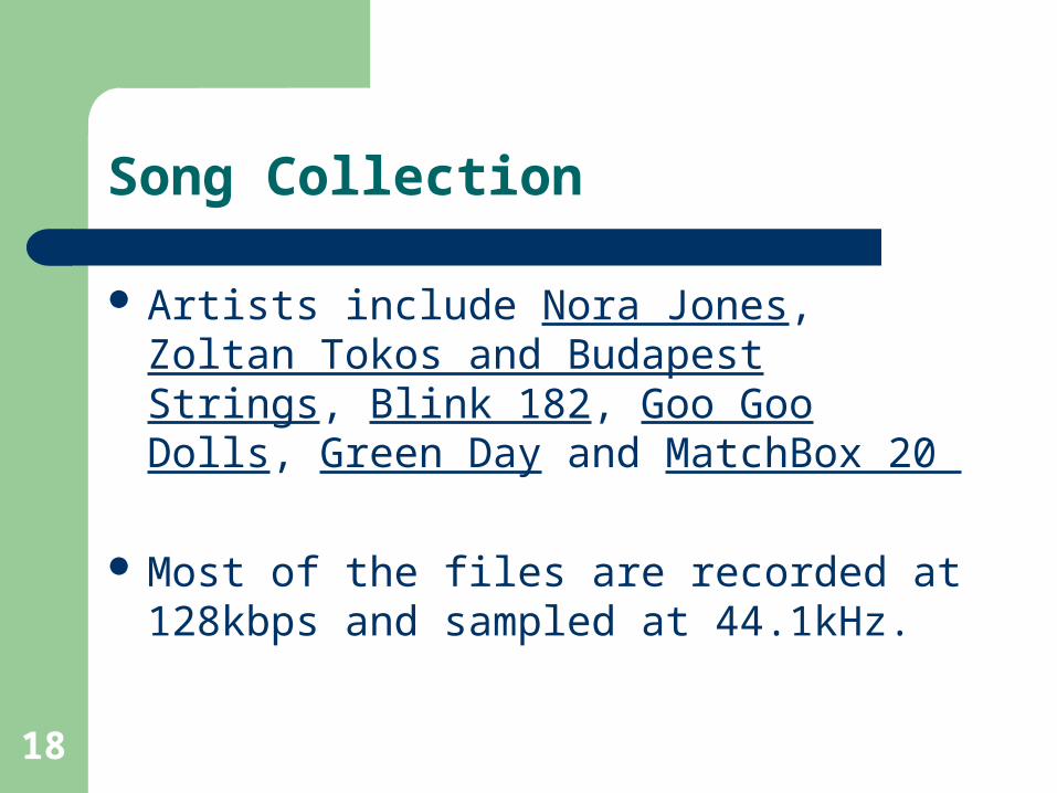
Song Collection
Artists include Nora Jones, Zoltan Tokos and Budapest Strings, Blink 182, Goo Goo Dolls, Green Day and MatchBox 20
Most of the files are recorded at 128kbps and sampled at 44.1kHz.

19
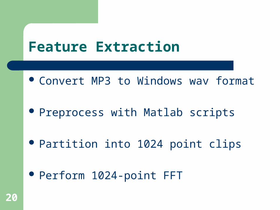
Feature Extraction
Process flow
MP3 WAVConversion Utility
.
.
.
.FFT
Partition the file into n-second clips
.
.
.
. Input Vectors
20
Feature Extraction
Convert MP3 to Windows wav format
Preprocess with Matlab scripts
Partition into 1024 point clips
Perform 1024-point FFT
21
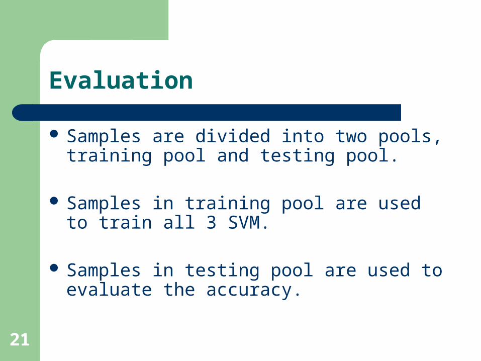
Evaluation
Samples are divided into two pools, training pool and testing pool.
Samples in training pool are used to train all 3 SVM.
Samples in testing pool are used to evaluate the accuracy.
22
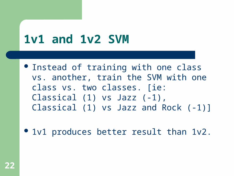
1v1 and 1v2 SVM
Instead of training with one class vs. another, train the SVM with one class vs. two classes. [ie: Classical (1) vs Jazz (-1), Classical (1) vs Jazz and Rock (-1)]
1v1 produces better result than 1v2.
23
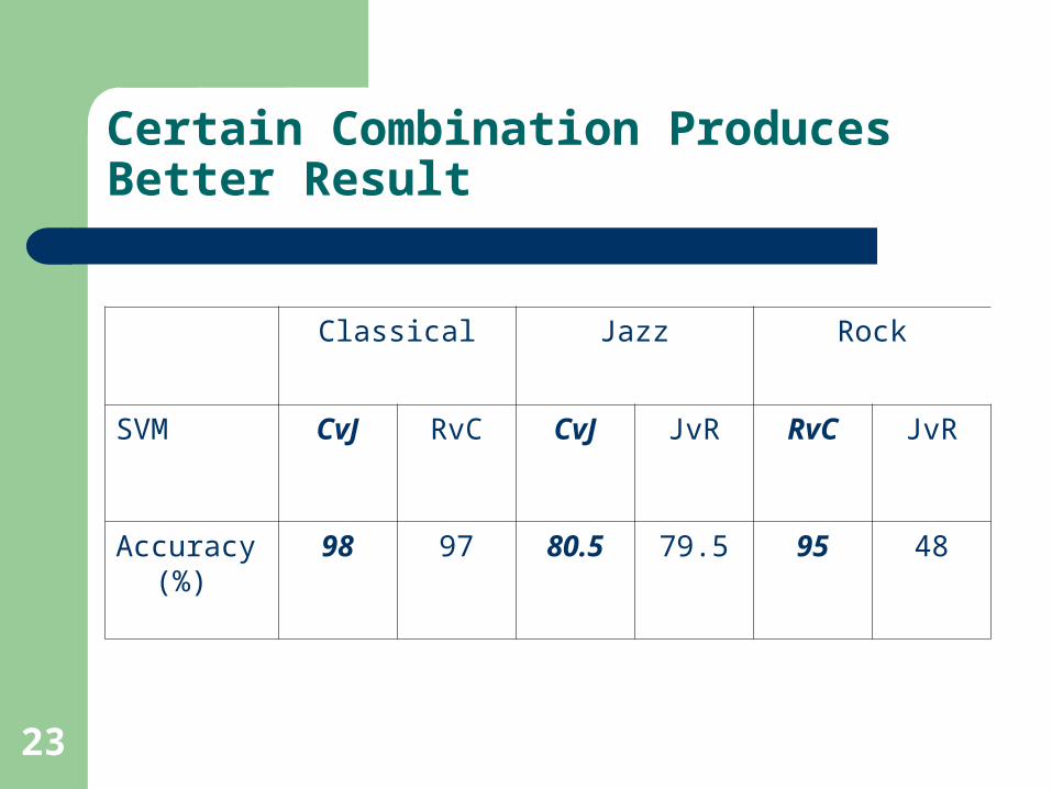
Certain Combination Produces Better Result
Classical Jazz Rock
SVM CvJ RvC CvJ JvR RvC JvR
Accuracy (%)
98 97 80.5 79.5 95 48
24
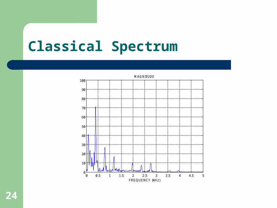
Classical Spectrum
0 0.5 1 1.5 2 2.5 3 3.5 4 4.5 50
10
20
30
40
50
60
70
80
90
100MAGNITUDE
FREQUENCY (kHz)
25
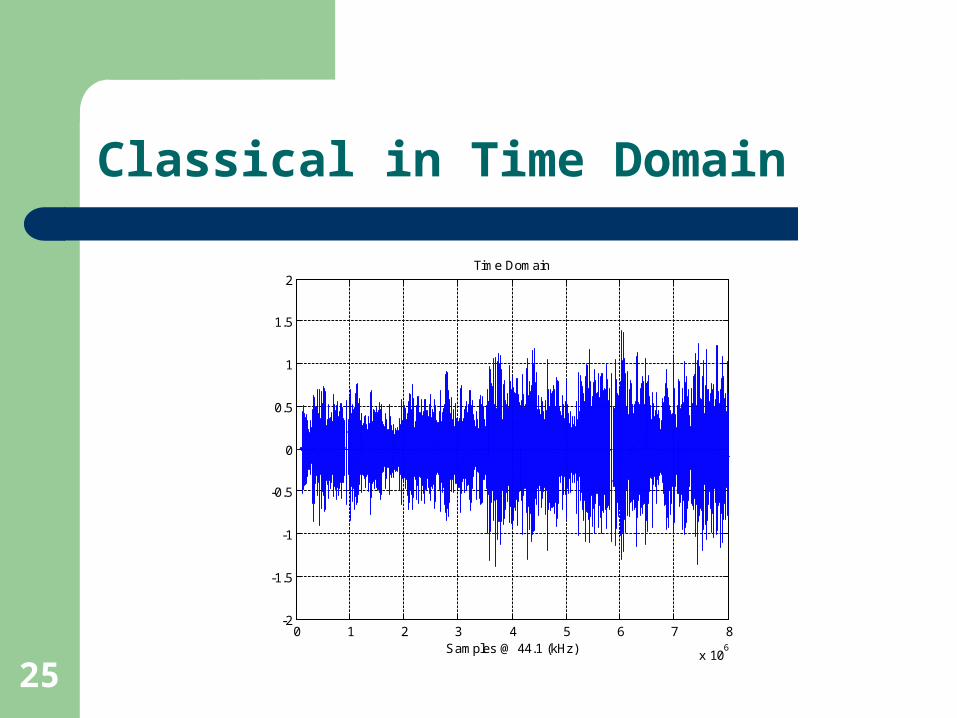
Classical in Time Domain
0 1 2 3 4 5 6 7 8
x 106
-2
-1.5
-1
-0.5
0
0.5
1
1.5
2Time Domain
Samples @ 44.1 (kHz)
26
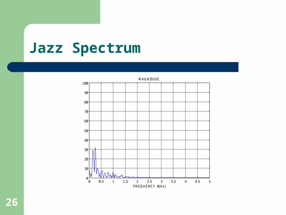
Jazz Spectrum
0 0.5 1 1.5 2 2.5 3 3.5 4 4.5 50
10
20
30
40
50
60
70
80
90
100MAGNITUDE
FREQUENCY (kHz)
27
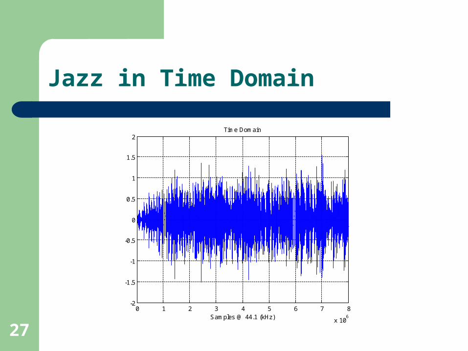
Jazz in Time Domain
0 1 2 3 4 5 6 7 8
x 106
-2
-1.5
-1
-0.5
0
0.5
1
1.5
2Time Domain
Samples @ 44.1 (kHz)
28
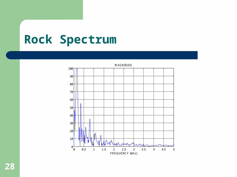
Rock Spectrum
0 0.5 1 1.5 2 2.5 3 3.5 4 4.5 50
10
20
30
40
50
60
70
80
90
100MAGNITUDE
FREQUENCY (kHz)
29
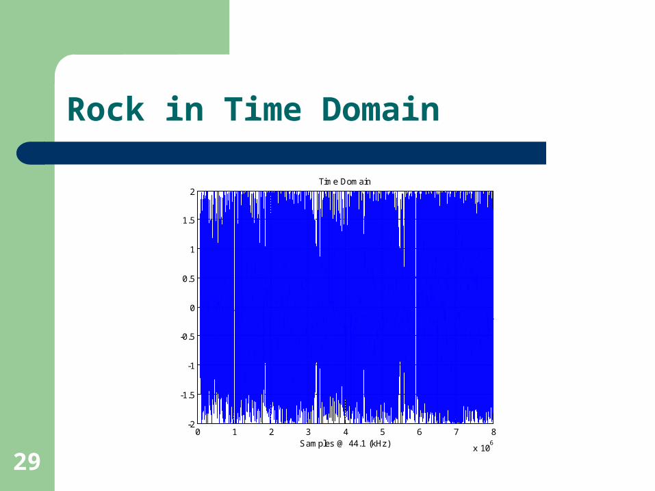
Rock in Time Domain
0 1 2 3 4 5 6 7 8
x 106
-2
-1.5
-1
-0.5
0
0.5
1
1.5
2Time Domain
Samples @ 44.1 (kHz)

30
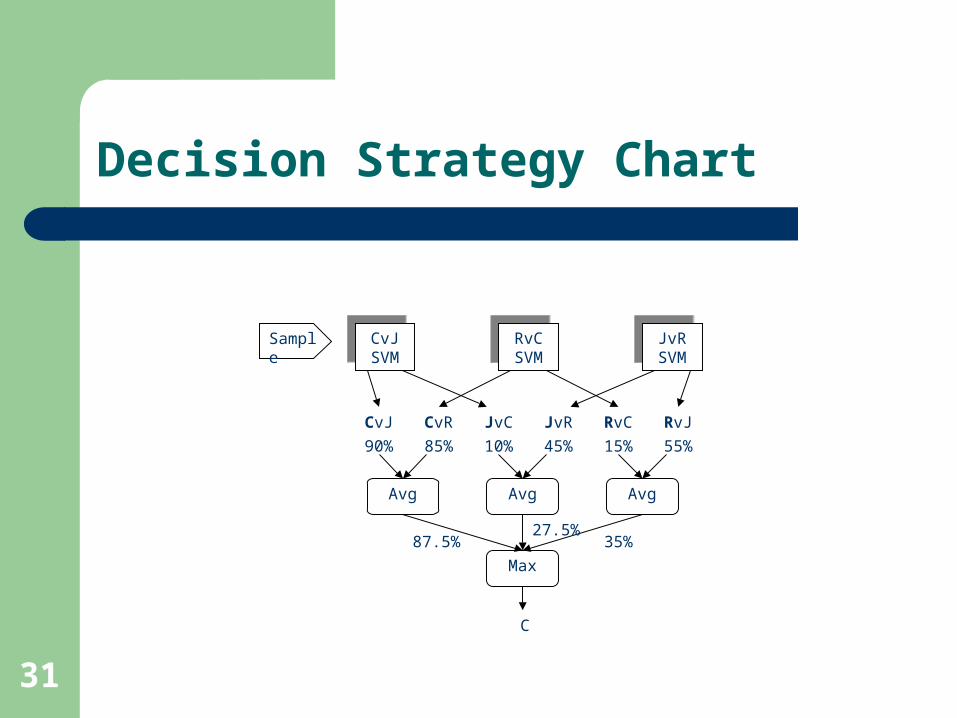
Sample-Set Method
1 sample-set = 100 individual samples
Average the scores for each class
Take the class of maximum as the classifier
31
Decision Strategy Chart
C
CvJ CvR JvC JvR RvC RvJ
CvJ SVM
CvJ SVM
RvC SVM
RvC SVM
JvR SVM
JvR SVM
Sample
90% 85% 10% 45% 15% 55%
Avg Avg Avg
Max
87.5%27.5%
35%
32
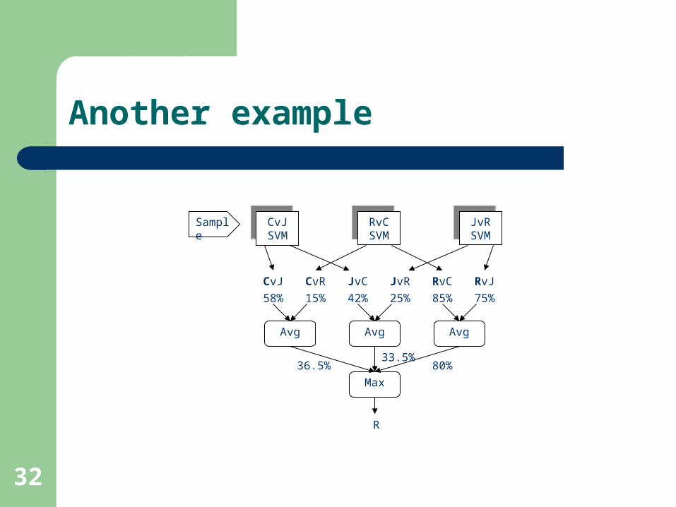
Another example
R
CvJ CvR JvC JvR RvC RvJ
CvJ SVM
CvJ SVM
RvC SVM
RvC SVM
JvR SVM
JvR SVM
Sample
58% 15% 42% 25% 85% 75%
Avg Avg Avg
Max
36.5%33.5%
80%
33
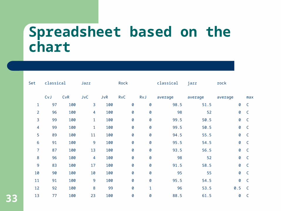
Spreadsheet based on the chart
Set classical Jazz Rock classical jazz rock
CvJ CvR JvC JvR RvC RvJ average average average max
1 97 100 3 100 0 0 98.5 51.5 0 C
2 96 100 4 100 0 0 98 52 0 C
3 99 100 1 100 0 0 99.5 50.5 0 C
4 99 100 1 100 0 0 99.5 50.5 0 C
5 89 100 11 100 0 0 94.5 55.5 0 C
6 91 100 9 100 0 0 95.5 54.5 0 C
7 87 100 13 100 0 0 93.5 56.5 0 C
8 96 100 4 100 0 0 98 52 0 C
9 83 100 17 100 0 0 91.5 58.5 0 C
10 90 100 10 100 0 0 95 55 0 C
11 91 100 9 100 0 0 95.5 54.5 0 C
12 92 100 8 99 0 1 96 53.5 0.5 C
13 77 100 23 100 0 0 88.5 61.5 0 C

34
Individual Result
600 Samples Classical Jazz Rock
Classical 196 41 10
Jazz 4 159 0
Roc 0 0 190
Accuracy 98% 79.5% 95%
35
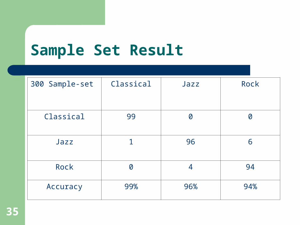
Sample Set Result
300 Sample-set Classical Jazz Rock
Classical 99 0 0
Jazz 1 96 6
Rock 0 4 94
Accuracy 99% 96% 94%
36
Other Algorithms
Neural Network
Gaussian Classifier
Hidden Markov Model
37
Gaussian Classifier [7]
Feature vector used is a conglomeration of different types of features. (mean-centroid, mean-rolloff, mean-flux, mean-zero-crossing, std-centroid, std-rolloff, std-flux, std-zero-crossing and LowEnergy)
6 genres, Classical, Country, Disco, Hiphop, Jazz, Rock.
Each classifier is trained by 50 samples each 30 seconds in length.
38
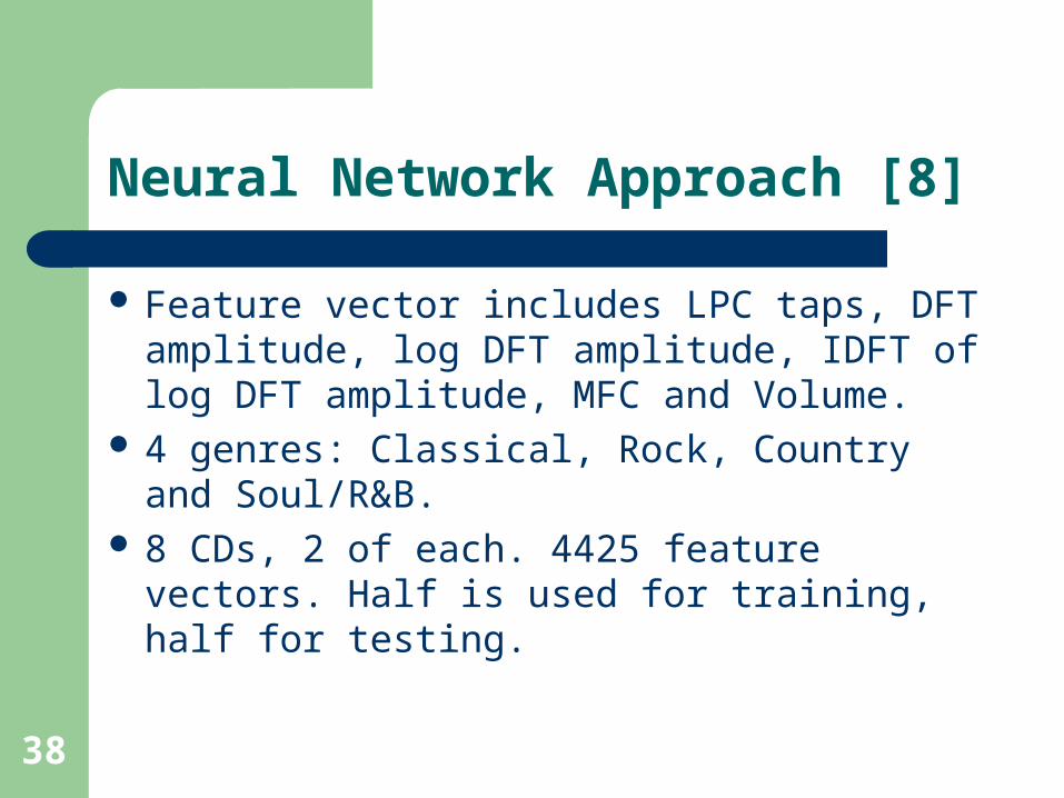
Neural Network Approach [8]
Feature vector includes LPC taps, DFT amplitude, log DFT amplitude, IDFT of log DFT amplitude, MFC and Volume.
4 genres: Classical, Rock, Country and Soul/R&B.
8 CDs, 2 of each. 4425 feature vectors. Half is used for training, half for testing.
39
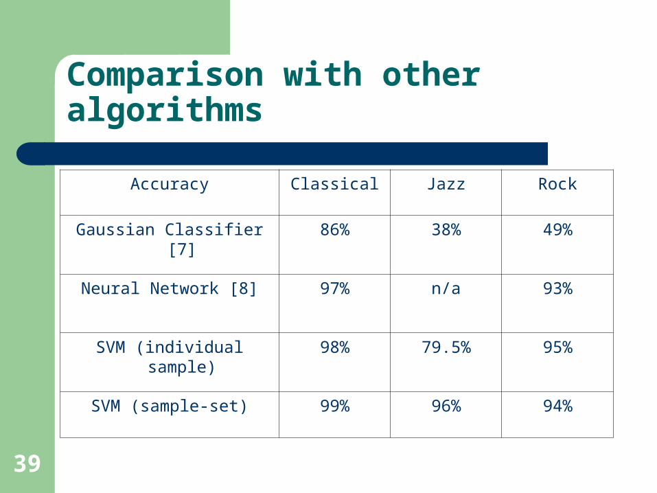
Comparison with other algorithms
Accuracy Classical Jazz Rock
Gaussian Classifier [7] 86% 38% 49%
Neural Network [8] 97% n/a 93%
SVM (individual sample) 98% 79.5% 95%
SVM (sample-set) 99% 96% 94%
40
Summary
Sample-Set method produces better result than individual samples.
SVM results are comparable to Neural Network results
Only used one feature
41
Other Applications of SVM
Optical Character Recognition Hand-Writing Recognition Image Classification Voice Recognition Protein Structure Prediction

42
Conclusion
Viable approach for music classification
More distinct features
Larger scale evaluation
Possible embedded application

43
Questions ???