SVM and Its Related Applications

Jung-Ying Wang

5/24/2006

2

Outline

• Basic concept of SVM• SVC formulations• Kernel function• Model selection (tuning SVM hyperparameters)• SVM application: breast cancer diagnosis• Prediction of protein secondary structure• SVM application in protein fold assignment

3

• Data classification

– training– testing

• Learning

– supervised learning (classification)– unsupervised learning (clustering)

Introduction

4

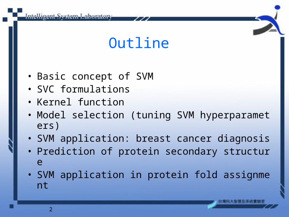
• Consider linear separable case• Training data two classes

0 bxT w

hyperplane Separating

Basic Concept of SVM

5

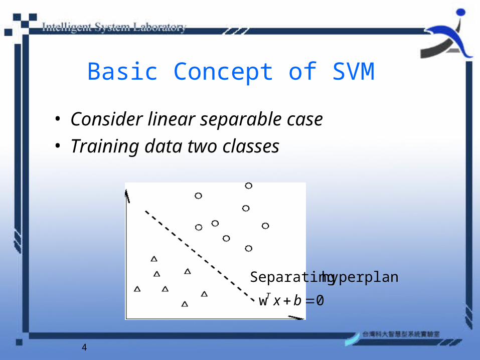
constant:b

tcoefficien:w

0623

6322

3

20

03

2

0

:

0:2

0 w

: hyperplane a ofEquation

2211

yx

xyx

y

example

bxwxwD

bxT

6

• f(x) > 0 class 1• f(x) < 0 class 2• How to find good w and b?• There are many possible (w,b)

bxwxf T )(

Decision Function

7

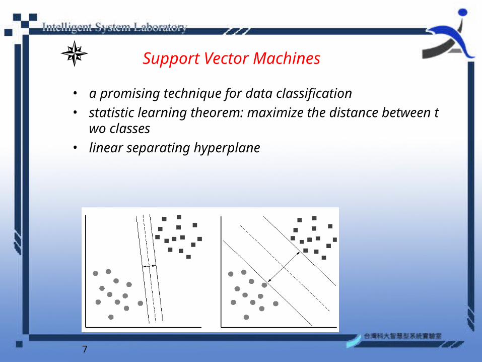
• a promising technique for data classification • statistic learning theorem: maximize the distance between t

wo classes• linear separating hyperplane

Support Vector Machines

8

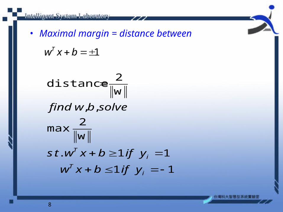
• Maximal margin = distance between

1 bxwT

11

11..

max

,,

iT

iT

yifbxw

yifbxwts

solvebwfind

w

2

w

2distance

9

• 1. How to solve w,b?• 2. Linear nonseparable case• 3. Is this (w,b) good?• 4. Multiple-class case

Questions?

10

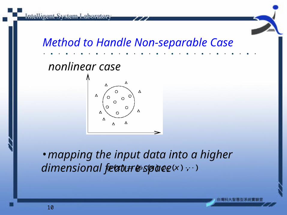
nonlinear case

•mapping the input data into a higher dimensional feature space )),(),(()( 21 xxx

Method to Handle Non-separable Case

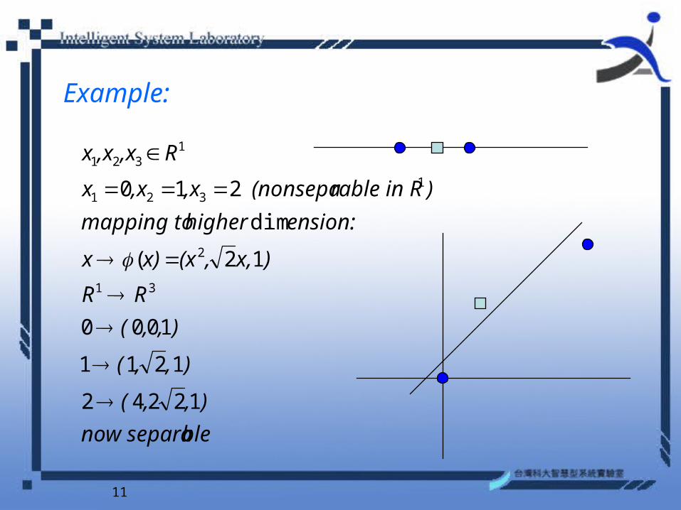
11

blenow separa

),,(

),,(

),,(

RR

)x,,(xx)x

ension: higher mapping to

)rable in R (nonsepa,x,xx

R,x,xx

12242

1211

1000

12(

dim

210

31

2

1321

1321

Example:

12

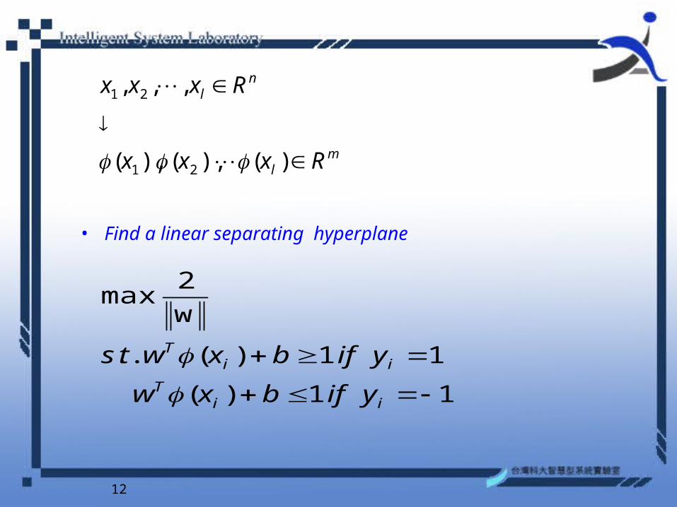
• Find a linear separating hyperplane

ml

nl

Rxxx

Rxxx

)(),(),(

,,,

21

21

11)(

11)(..

max

iiT

iiT

yifbxw

yifbxwts

w

2

13

libxwytosubject

ww

iT

i

T

bw

,11))((..

2min

2minmax ,

w

w

2

• Questions:• 1. How to choose ?• 2. Is it really better? Yes.• Some times even in high dimension spaces. Data

may still not separable.

Allow training error

14

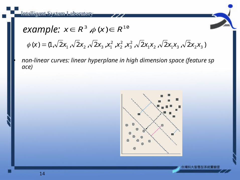
)2,2,2,,,,2,2,2,1()( 32312123

22

21321 xxxxxxxxxxxxx

103 )(, RxRx example:

• non-linear curves: linear hyperplane in high dimension space (feature space)

15

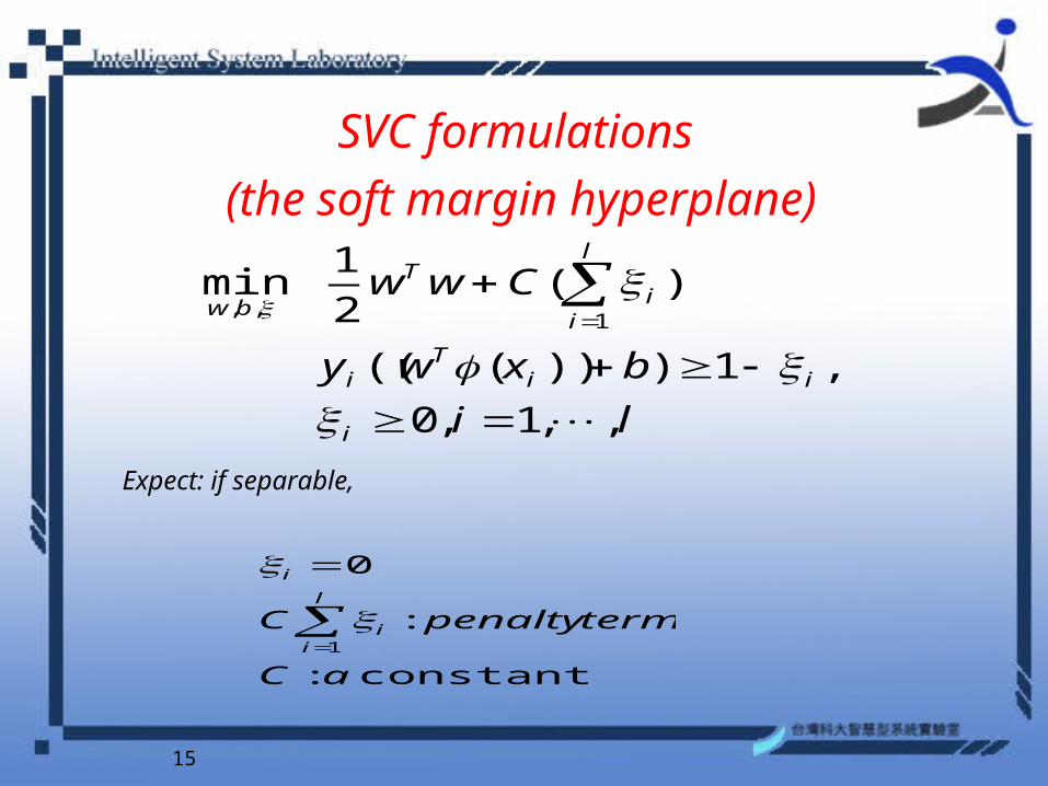
Expect: if separable,

constant:

:

0

1

aC

termpenaltyCl

ii

i

li

bxwy

Cww

i

iiT

i

l

ii

T

bw

,,1,0

,1)))(((

)(2

1min

1,,

SVC formulations

(the soft margin hyperplane)

16

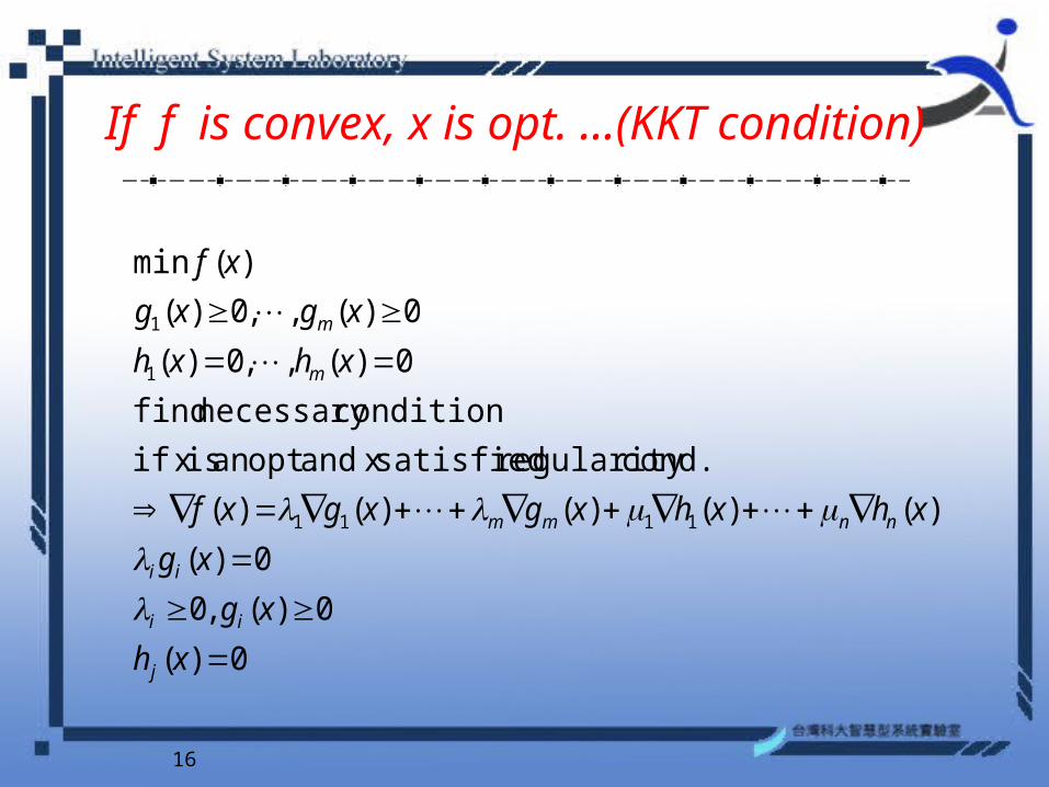
0)(

0)(,0

0)(

)()()()()(

cond. regularity satisfied x and opt.an is x if

conditionnecessary find

0)(,,0)(

0)(,,0)(

)(min

1111

1

1

xh

xg

xg

xhxhxgxgxf

xhxh

xgxg

xf

j

ii

ii

nnmm

m

m

If f is convex, x is opt. …(KKT condition)

17

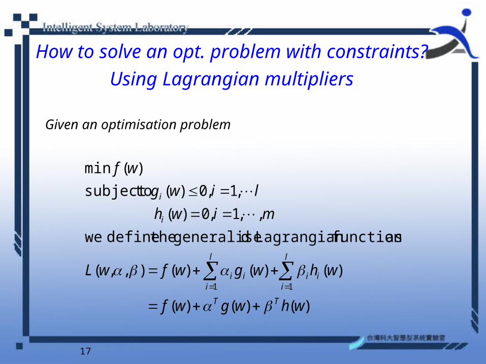
Given an optimisation problem

)()()(

)()()(),,(

,,1,0)(

,1,0)(

)(min

11

whwgwf

whwgwfwL

miwh

liwg

wf

TT

l

iii

l

iii

i

i

as function Lagrangian dgeneralise the define we

to subject

How to solve an opt. problem with constraints?

Using Lagrangian multipliers

18

• Consider the following primal problem: 

 

• (P) # variables: w dimension of (x) ( very big number) , b1, l

• (D) # variables: l• Derive its dual.

li

libxwytosubject

Cww

i

iiT

i

l

ii

Tbw

,,1,0

,,1,1))((

1,,

minimise

What is good in Dual than Primal?

19

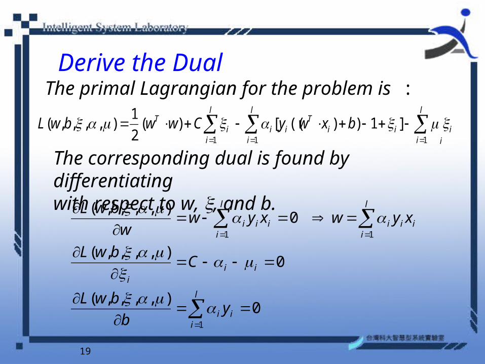
 Derive the DualThe primal Lagrangian for the problem is :

ii

l

ii

l

ii

Tii

l

ii

T bxwyCwwbwL

111

]1))(([)(2

1),,,,(

l

iii

iii

l

iiii

l

iiii

yb

bwL

CbwL

xywxyww

bwL

1

11

0),,,,(

0),,,,(

0),,,,(

The corresponding dual is found by differentiating with respect to w, , and b.

20

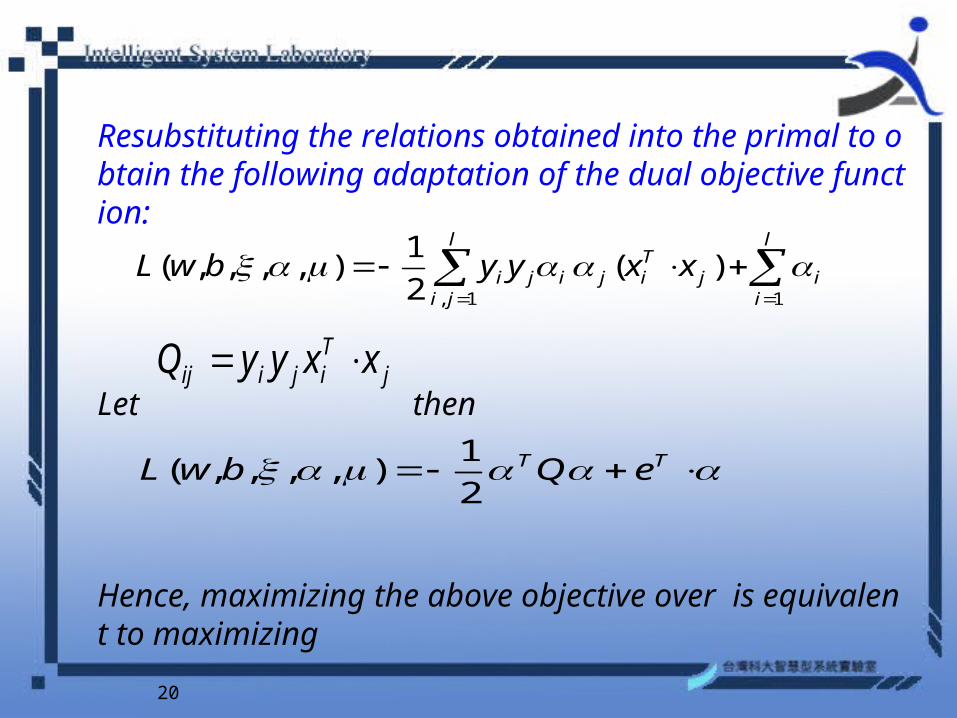
Resubstituting the relations obtained into the primal to obtain the following adaptation of the dual objective function:  

Let then

 Hence, maximizing the above objective over is equivalent to maximizing 

l

ii

l

jij

Tijiji xxyybwL

11,

)(2

1),,,,(

jTijiij xxyyQ

TT eQbwL2

1),,,,(

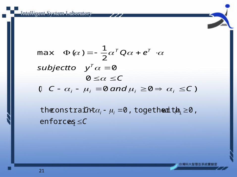
21

)00(

0

0

2

1)(max

CandC

C

ytosubject

eQ

iiii

T

TT

C

C ii

i

i

enforces

, 0 with together , 0 constraint the

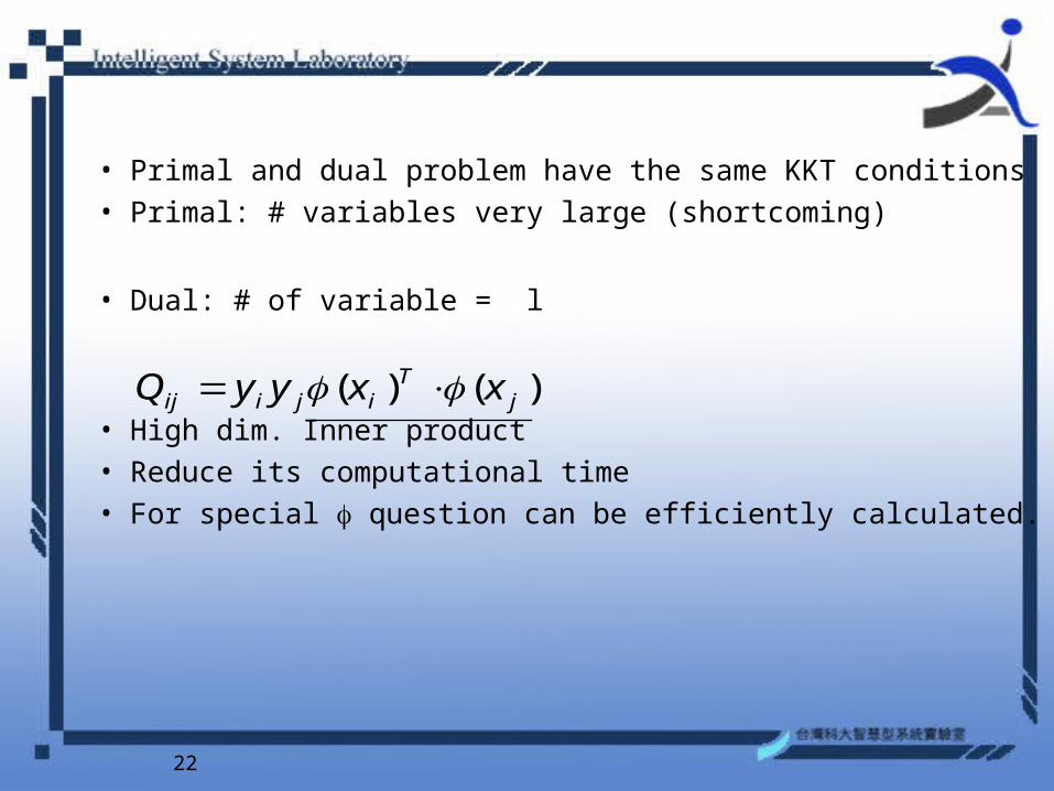
22

• Primal and dual problem have the same KKT conditions• Primal: # variables very large (shortcoming)

• Dual: # of variable = l

• High dim. Inner product• Reduce its computational time• For special question can be efficiently calculated.

)()( jT

ijiij xxyyQ

23

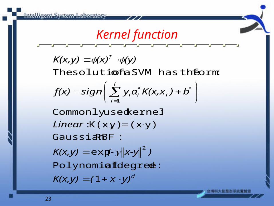
Kernel function

l

i

*i

*ii

T

b)K(x,xαysign f(x)

(y)(x)K(x,y)

1

:form thehas SVM a ofsolution The

dy)x(K(x,y)

)x-y(-K(x,y)

Linear

1

:ddegree of Polynomial

exp

:RBFGaussian

: kernels usedCommonly

2

y)(xy)K(x, :

24

Kernel function

dy)x(K(x,y)

)x-y(-K(x,y)

Linear

1

:ddegree of Polynomial

exp

:RBFGaussian

: kernels usedCommonly

2

y)(xy)K(x, :

25

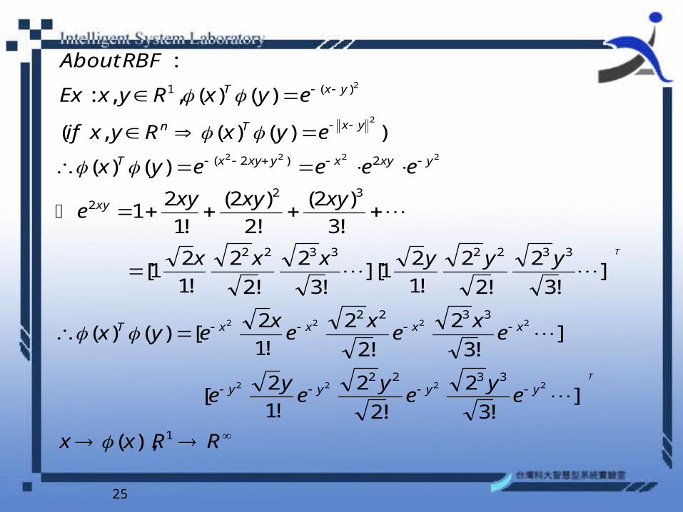
RRxx

ey

ey

ey

e

ex

ex

ex

eyx

yyyxxx

xyxyxye

eeeeyx

eyxRyxif

eyxRyxEx

RBFAbout

T

T

yyyy

xxxxT

xy

yxyxyxyxT

yxTn

yxT

1

3322

3322

33223322

322

2)2(

)(1

),(

]!3

2

!2

2

!1

2[

]!3

2

!2

2

!1

2[)()(

]!3

2

!2

2

!1

21[]

!3

2

!2

2

!1

21[

!3

)2(

!2

)2(

!1

21

)()(

))()(,(

)()(,,:

:

2222

2222

2222

2

2

26

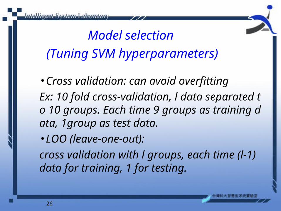
Model selection

(Tuning SVM hyperparameters)

•Cross validation: can avoid overfitting

Ex: 10 fold cross-validation, l data separated to 10 groups. Each time 9 groups as training data, 1group as test data.•LOO (leave-one-out):

cross validation with l groups, each time (l-1) data for training, 1 for testing.

27

Model Selection

• The commonly used method of the model selection is grid method

28

Model Selection of SVMs Using GA Approach

• Peng-Wei Chen, Jung-Ying Wang  and Hahn-Ming Lee;  2004 IJCNN International Joint Conference on Neural Networks, 26 - 29 July 2004.

• Abstract— A new automatic search methodology for model selection of support vector machines, based on the GA-based tuning algorithm, is proposed to search for

the adequate hyperameters of SVMs.

29

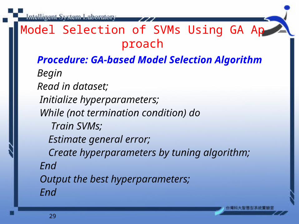
Model Selection of SVMs Using GA Approach

Procedure: GA-based Model Selection AlgorithmBegin Read in dataset; Initialize hyperparameters; While (not termination condition) do

Train SVMs; Estimate general error; Create hyperparameters by tuning algorithm; End Output the best hyperparameters; End

30

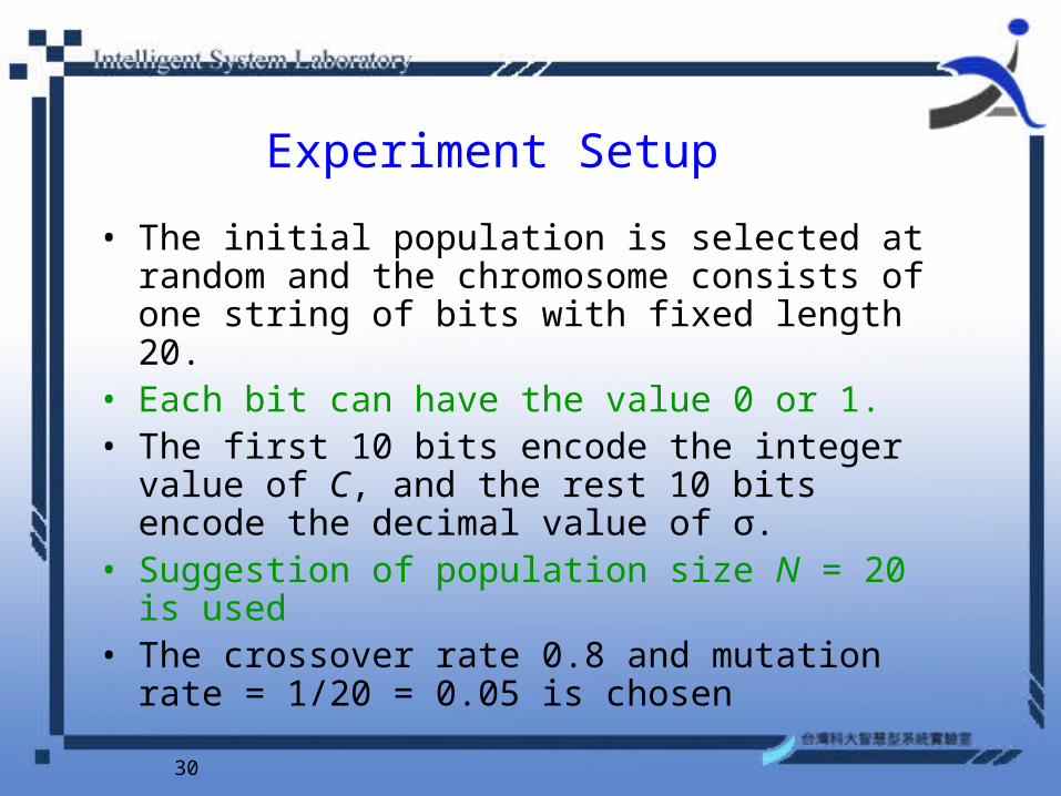
Experiment Setup • The initial population is selected at random and the

chromosome consists of one string of bits with fixed length 20.

• Each bit can have the value 0 or 1.• The first 10 bits encode the integer value of C, and

the rest 10 bits encode the decimal value of σ.• Suggestion of population size N = 20 is used • The crossover rate 0.8 and mutation rate = 1/20 =

0.05 is chosen

31

SVM Application: Breast Cancer Diagnosis  Software WEKA

32

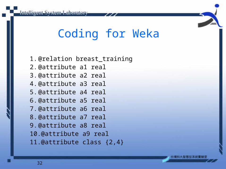
Coding for Weka

1. @relation breast_training2. @attribute a1 real3. @attribute a2 real4. @attribute a3 real5. @attribute a4 real6. @attribute a5 real7. @attribute a6 real8. @attribute a7 real9. @attribute a8 real10.@attribute a9 real11.@attribute class {2,4}

33

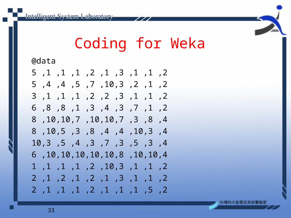
Coding for Weka@data

5 ,1 ,1 ,1 ,2 ,1 ,3 ,1 ,1 ,2

5 ,4 ,4 ,5 ,7 ,10,3 ,2 ,1 ,2

3 ,1 ,1 ,1 ,2 ,2 ,3 ,1 ,1 ,2

6 ,8 ,8 ,1 ,3 ,4 ,3 ,7 ,1 ,2

8 ,10,10,7 ,10,10,7 ,3 ,8 ,4

8 ,10,5 ,3 ,8 ,4 ,4 ,10,3 ,4

10,3 ,5 ,4 ,3 ,7 ,3 ,5 ,3 ,4

6 ,10,10,10,10,10,8 ,10,10,4

1 ,1 ,1 ,1 ,2 ,10,3 ,1 ,1 ,2

2 ,1 ,2 ,1 ,2 ,1 ,3 ,1 ,1 ,2

2 ,1 ,1 ,1 ,2 ,1 ,1 ,1 ,5 ,2

34

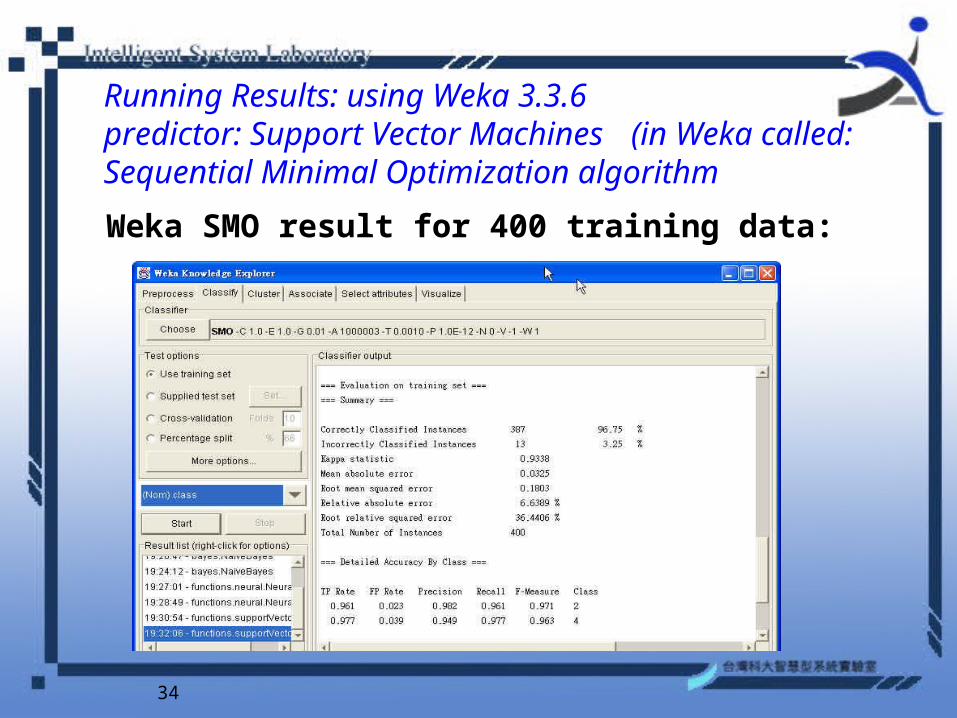
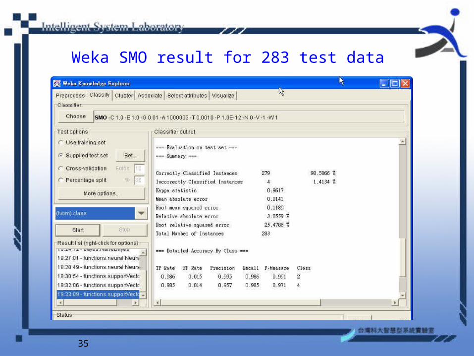
Running Results: using Weka 3.3.6 predictor: Support Vector Machines  (in Weka called: Sequential Minimal Optimization algorithm

Weka SMO result for 400 training data:

35

Weka SMO result for 283 test data

36

Software and Model Selection

• software: LIBSVM

• mapping function: use Radial Basis Function

• find the best parameter C and kernel parameter

• use cross validation to do the model selection

37

LIBSVM Model Selection using Grid Method

-c 1000 -g 10 3-fold accuracy= 69.8389-c 1000 -g 1000 3-fold accuracy= 69.8389-c 1 -g 0.002 3-fold accuracy= 97.0717 winner-c 1 -g 0.004 3-fold accuracy= 96.9253

38

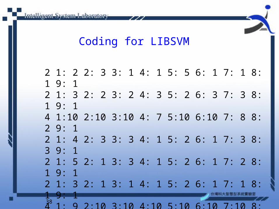
Coding for LIBSVM

2 1: 2 2: 3 3: 1 4: 1 5: 5 6: 1 7: 1 8: 1 9: 1 2 1: 3 2: 2 3: 2 4: 3 5: 2 6: 3 7: 3 8: 1 9: 1 4 1:10 2:10 3:10 4: 7 5:10 6:10 7: 8 8: 2 9: 1 2 1: 4 2: 3 3: 3 4: 1 5: 2 6: 1 7: 3 8: 3 9: 1 2 1: 5 2: 1 3: 3 4: 1 5: 2 6: 1 7: 2 8: 1 9: 1 2 1: 3 2: 1 3: 1 4: 1 5: 2 6: 1 7: 1 8: 1 9: 1 4 1: 9 2:10 3:10 4:10 5:10 6:10 7:10 8:10 9: 1 2 1: 5 2: 3 3: 6 4: 1 5: 2 6: 1 7: 1 8: 1 9: 1 4 1: 8 2: 7 3: 8 4: 2 5: 4 6: 2 7: 5 8:10 9: 1

39

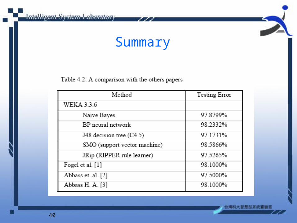
Summary

40

Summary

41

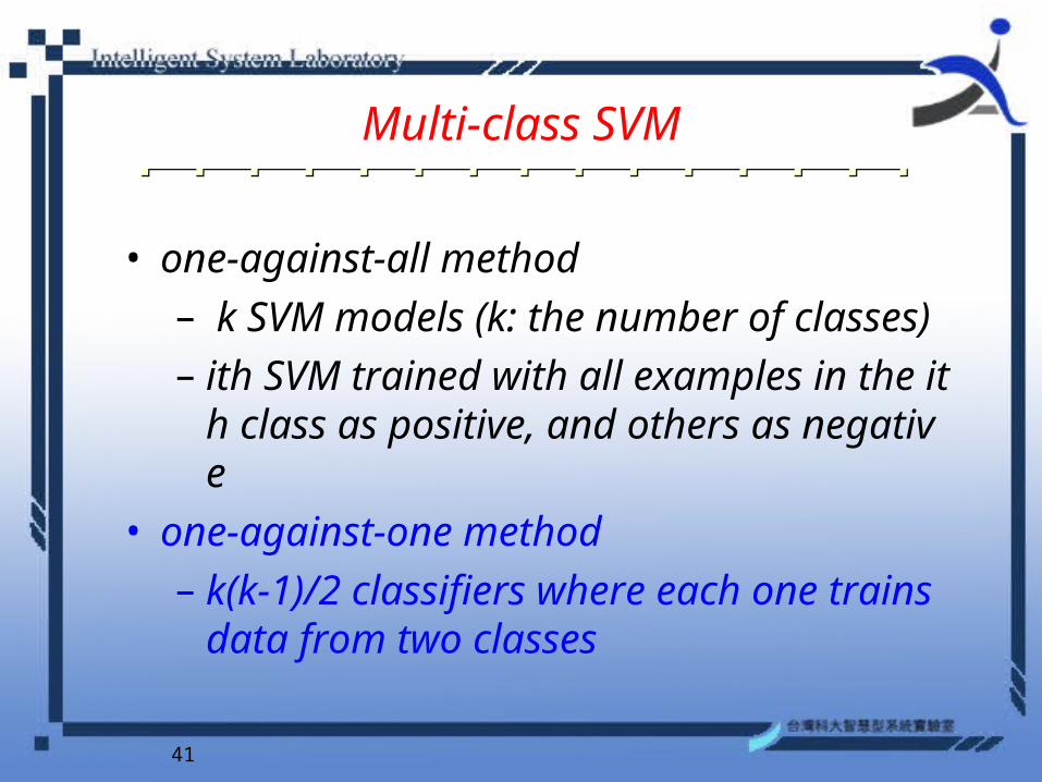
Multi-class SVM

• one-against-all method

– k SVM models (k: the number of classes)

– ith SVM trained with all examples in the ith class as positive, and others as negative

• one-against-one method

– k(k-1)/2 classifiers where each one trains data from two classes

42

SVM Application in Bioinformatics

• Prediction of protein secondary structure

• SVM application in protein fold assignment

43

Introduction to Secondary Structure

• The prediction of protein secondary structure is an important step to determine structural properties of proteins.

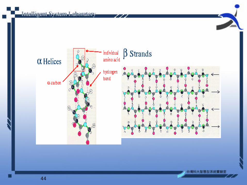
• The secondary structure consists of local folding regularities maintained by hydrogen bonds and is traditionally subdivided into three classes: alpha-helices, beta-sheets, and coil.

44

45

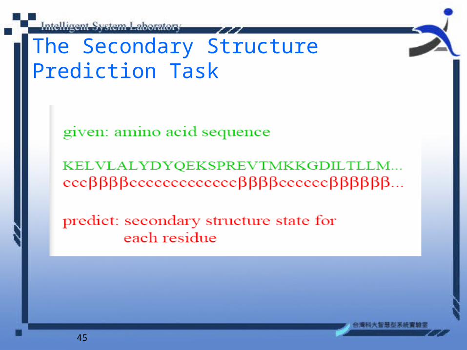
The Secondary Structure Prediction Task

46

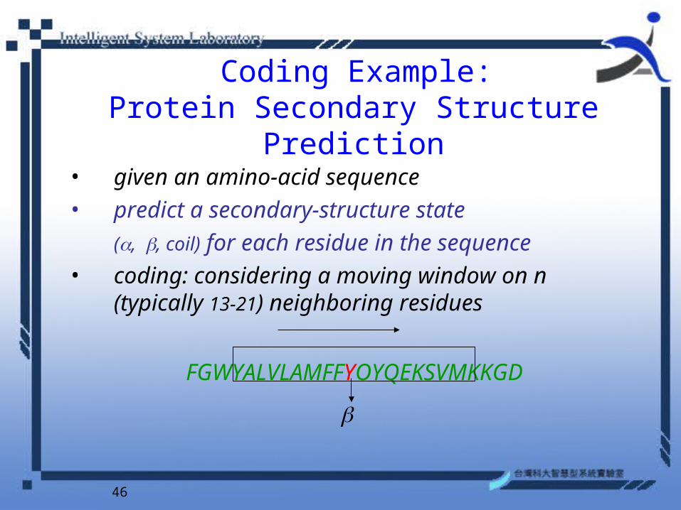
Coding Example:Protein Secondary Structure Prediction

• given an amino-acid sequence • predict a secondary-structure state

(,, coil) for each residue in the sequence• coding: considering a moving window on n (typically

13-21) neighboring residues

FGWYALVLAMFFYOYQEKSVMKKGD

47

Methods

1. statistical information ( Figureau et al., 2003; Yan et al., 2004);

2. neural networks (Qian and Sejnowski, 1988; Rost and Sander, 1993;; Pollastri et al., 2002; Cai et al., 2003; Kaur and Raghava, 2004; Wood and Hirst, 2004; Lin et al., 2005);

3. nearest-neighbor algorithms

4. hidden Markov modes

5. support vector machines (Hua and Sun, 2001; Hyunsoo and Haesun, 2003; Ward et al., 2003; Guo et al., 2004).

48

Milestone

• In 1988, using Neural Networks first achieved about 62% accuracy (Qian and Sejnowski, 1988; Holley and Karplus, 1989).

• In 1993, using evolutionary information, Neural Network system had improved the prediction accuracy to over 70% (Rost and Sander, 1993).

• Recently there have been approaches (e.g. Baldi et al., 1999; Petersen et al., 2000; Pollastr and McLysaght, 2005) using neural networks which achieve even higher accuracy (> 78%).

49

Benchmark (Data Set Used in Protein Secondary Structure)

• Rost and Sander data set (Rost and Sander, 1993) (referred as RS126)

• Note that the RS126 data set consists of 25,184 data points in three classes where 47% are coil, 32% are helix, and 21% are strand.

• Cuff and Barton data set (Cuff and Barton, 1999) (referred as CB513)

• The performance accuracy is verified by a 7-fold cross validation.

50

Secondary Structure Assignment

• According to the DSSP (Dictionary of Secondary Structures of Proteins) algorithm (Kabsch and Sander, 1983), which distinguishes eight secondary structure classes

• We converted the eight types into three classes in the following way: H (α-helix), I (π-helix), and G (310-helix) as helix (α), E (extended strand) as β-strand (β), and all others as coil (c).

• Different conversion methods influence the prediction accuracy to some extent, as discussed by Cutt and Barton (Cutt and Barton, 1999).

51

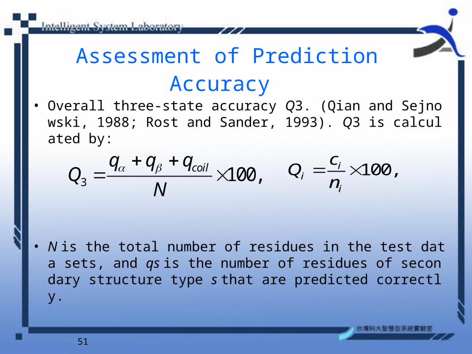
Assessment of Prediction Accuracy

• Overall three-state accuracy Q3. (Qian and Sejnowski, 1988; Rost and Sander, 1993). Q3 is calculated by:

• N is the total number of residues in the test data sets, and qs is the number of residues of secondary structure type s that are predicted correctly.

3 100,coilq q qQ

N

100,ii

i

cQ

n

52

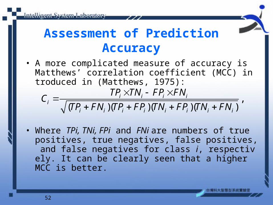
Assessment of Prediction Accuracy

• A more complicated measure of accuracy is Matthews’ correlation coefficient (MCC) introduced in (Matthews, 1975):

• Where TPi, TNi, FPi and FNi are numbers of true positives, true negatives, false positives, and false negatives for class i, respectively. It can be clearly seen that a higher MCC is better.

,( )( )( )( )

i i i ii

i i i i i i i i

TP TN FP FNC

TP FN TP FP TN FP TN FN

53

Support Vector Machines Predictor

• Using the software LIBSVM (Chang and Lin, 2005) as our SVM predictor

• Using the RBF kernel for all experiments

• Choosing optimal parameter for support vector machines. Find the pair of C = 10 and γ = 0.01 that achieves the best prediction rate

54

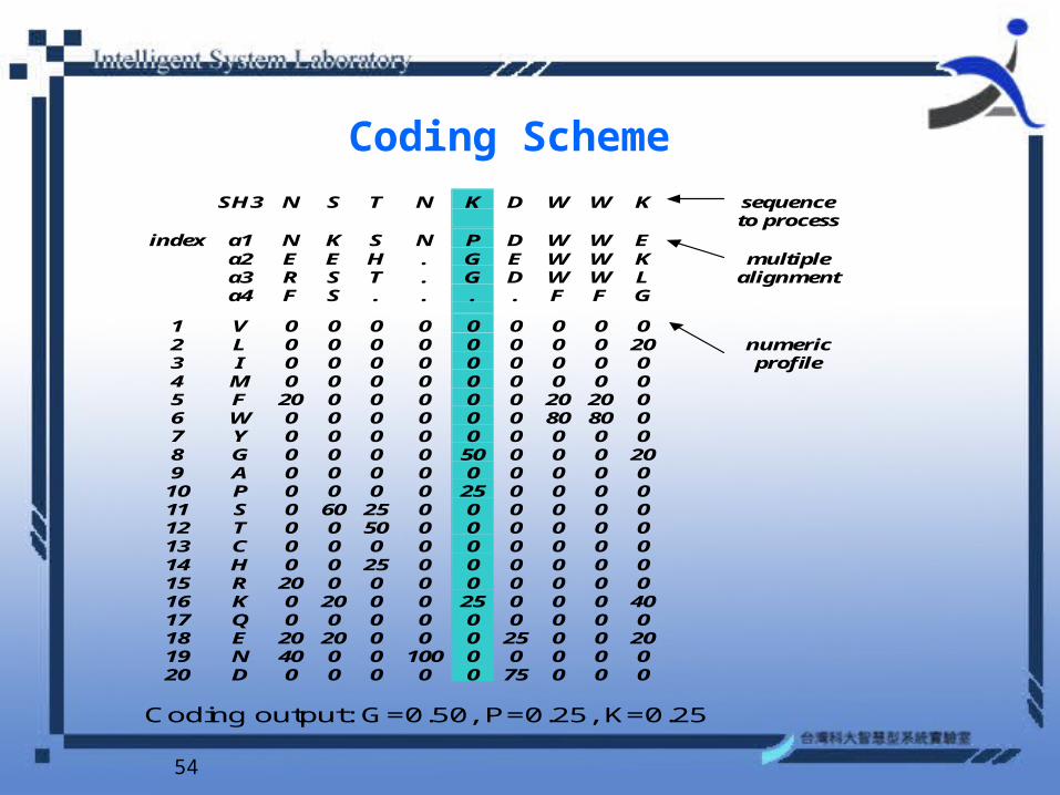
Coding Scheme SH3 N S T N K D W W K sequence to process

index a1 N K S N P D W W E a2 E E H . G E W W K multiple a3 R S T . G D W W L alignment a4 F S . . . . F F G

1 V 0 0 0 0 0 0 0 0 0 2 L 0 0 0 0 0 0 0 0 20 numeric 3 I 0 0 0 0 0 0 0 0 0 profile 4 M 0 0 0 0 0 0 0 0 0 5 F 20 0 0 0 0 0 20 20 0 6 W 0 0 0 0 0 0 80 80 0 7 Y 0 0 0 0 0 0 0 0 0 8 G 0 0 0 0 50 0 0 0 20 9 A 0 0 0 0 0 0 0 0 0 10 P 0 0 0 0 25 0 0 0 0 11 S 0 60 25 0 0 0 0 0 0 12 T 0 0 50 0 0 0 0 0 0 13 C 0 0 0 0 0 0 0 0 0 14 H 0 0 25 0 0 0 0 0 0 15 R 20 0 0 0 0 0 0 0 0 16 K 0 20 0 0 25 0 0 0 40 17 Q 0 0 0 0 0 0 0 0 0 18 E 20 20 0 0 0 25 0 0 20 19 N 40 0 0 100 0 0 0 0 0 20 D 0 0 0 0 0 75 0 0 0

Coding output: G=0.50, P=0.25, K=0.25

55

Coding Scheme for Support Vector Machines

• We use the BLASTP to generate the alignments (profile) of proteins in our database

• The expectation value (E-value) of 10.0 and choosing the non-redundant protein sequence database (NCBI nr database) to search.

• The profile data obtained from BLASTPGP are normalized to 0~1, and then used as inputs to our SVM predictor.

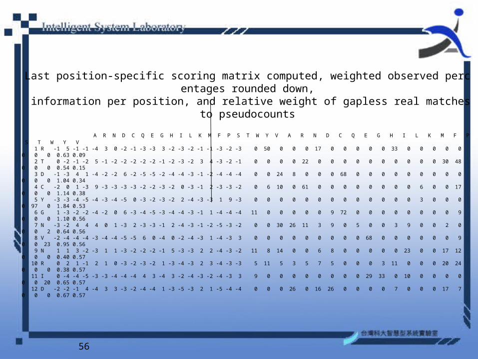
56

Last position-specific scoring matrix computed, weighted observed percentages rounded down, information per position, and relative weight of gapless real matches to pseudocounts

A R N D C Q E G H I L K M F P S T W Y V A R N D C Q E G H I L K M F P S T W Y V 1 R -1 5 -1 -1 -4 3 0 -2 -1 -3 -3 3 -2 -3 -2 -1 -1 -3 -2 -3 0 50 0 0 0 17 0 0 0 0 0 33 0 0 0 0 0 0 0 0 0.63 0.09 2 T 0 -2 -1 -2 5 -1 -2 -2 -2 -2 -2 -1 -2 -3 -2 3 4 -3 -2 -1 0 0 0 0 22 0 0 0 0 0 0 0 0 0 0 30 48 0 0 0 0.54 0.15 3 D -1 -3 4 1 -4 -2 -2 6 -2 -5 -5 -2 -4 -4 -3 -1 -2 -4 -4 -4 0 0 24 8 0 0 0 68 0 0 0 0 0 0 0 0 0 0 0 0 1.04 0.34 4 C -2 0 1 -3 9 -3 -3 -3 -3 -2 -2 -3 -2 0 -3 -1 2 -3 -3 -2 0 6 10 0 61 0 0 0 0 0 0 0 0 6 0 0 17 0 0 0 1.14 0.38 5 Y -3 -3 -4 -5 -4 -3 -4 -5 0 -3 -2 -3 -2 2 -4 -3 -3 1 9 -3 0 0 0 0 0 0 0 0 0 0 0 0 0 3 0 0 0 0 97 0 1.84 0.53 6 G 1 -3 -2 -2 -4 -2 0 6 -3 -4 -5 -3 -4 -4 -3 -1 1 -4 -4 -4 11 0 0 0 0 0 9 72 0 0 0 0 0 0 0 0 9 0 0 0 1.10 0.56 7 N -3 -2 4 4 4 0 1 -3 2 -3 -3 -1 2 -4 -3 -1 -2 -5 -3 -2 0 0 30 26 11 3 9 0 5 0 0 3 9 0 0 2 0 0 0 2 0.64 0.56 8 V -2 -4 -4 -4 -3 -4 -4 -5 -5 6 0 -4 0 -2 -4 -3 1 -4 -3 3 0 0 0 0 0 0 0 0 0 68 0 0 0 0 0 0 9 0 0 23 0.95 0.56 9 N 1 1 3 -2 -3 1 1 -3 -2 -2 -2 -1 5 -3 -3 2 2 -4 -3 -2 11 8 14 0 0 6 8 0 0 0 0 0 23 0 0 17 12 0 0 0 0.40 0.57 10 R 0 2 1 -1 2 1 0 -3 -2 -3 -2 1 -3 -4 -3 2 3 -4 -3 -3 5 11 5 3 5 7 5 0 0 0 3 11 0 0 0 20 24 0 0 0 0.38 0.57 11 I 0 -4 -4 -5 -3 -3 -4 -4 -4 4 3 -4 3 -2 -4 -3 -2 -4 -3 3 9 0 0 0 0 0 0 0 0 29 33 0 10 0 0 0 0 0 0 20 0.65 0.57 12 D -2 -2 -1 4 -4 3 3 -3 -2 -4 -4 1 -3 -5 -3 2 1 -5 -4 -4 0 0 0 26 0 16 26 0 0 0 0 7 0 0 0 17 7 0 0 0 0.67 0.57

57

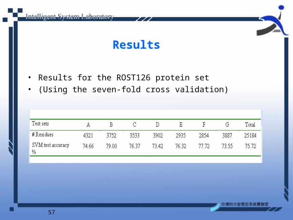
Results

• Results for the ROST126 protein set• (Using the seven-fold cross validation)

58

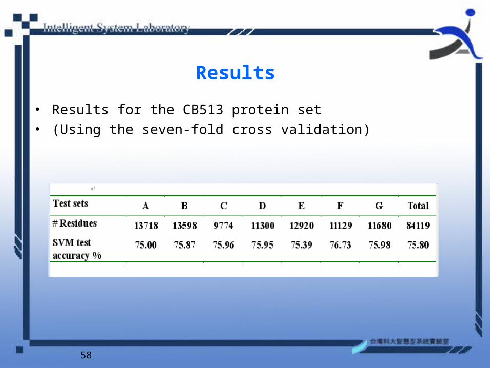
Results

• Results for the CB513 protein set• (Using the seven-fold cross validation)

59

SVM Application in Protein Fold Assignment

"Fine-grained Protein Fold Assignment by Support Vector Machines using generalized n-peptide Coding Schemes and jury voting from multiple parameter sets",

Chin-Sheng Yu, Jung-Ying Wang, Jin-Moon Young, P.-C. Lyu, Chih-Jen Lin, Jenn-Kang Hwang,

 Proteins: Structure, Function, Genetics, 50, 531-536 (2003).

60

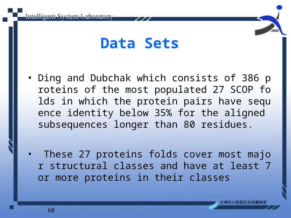
Data Sets

• Ding and Dubchak which consists of 386 proteins of the most populated 27 SCOP folds in which the protein pairs have sequence identity below 35% for the aligned subsequences longer than 80 residues.

• These 27 proteins folds cover most major structural classes and have at least 7 or more proteins in their classes

61

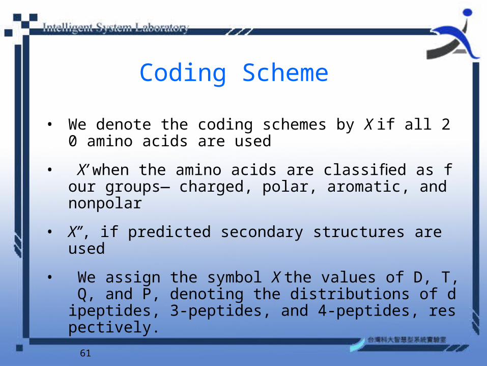
Coding Scheme

• We denote the coding schemes by X if all 20 amino acids are used

• X’ when the amino acids are classified as four groups— charged, polar, aromatic, and nonpolar

• X’’, if predicted secondary structures are used

• We assign the symbol X the values of D, T, Q, and P, denoting the distributions of dipeptides, 3-peptides, and 4-peptides, respectively.

62

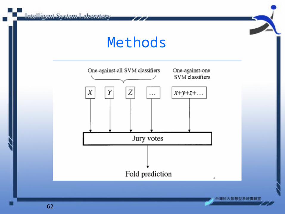
Methods

63

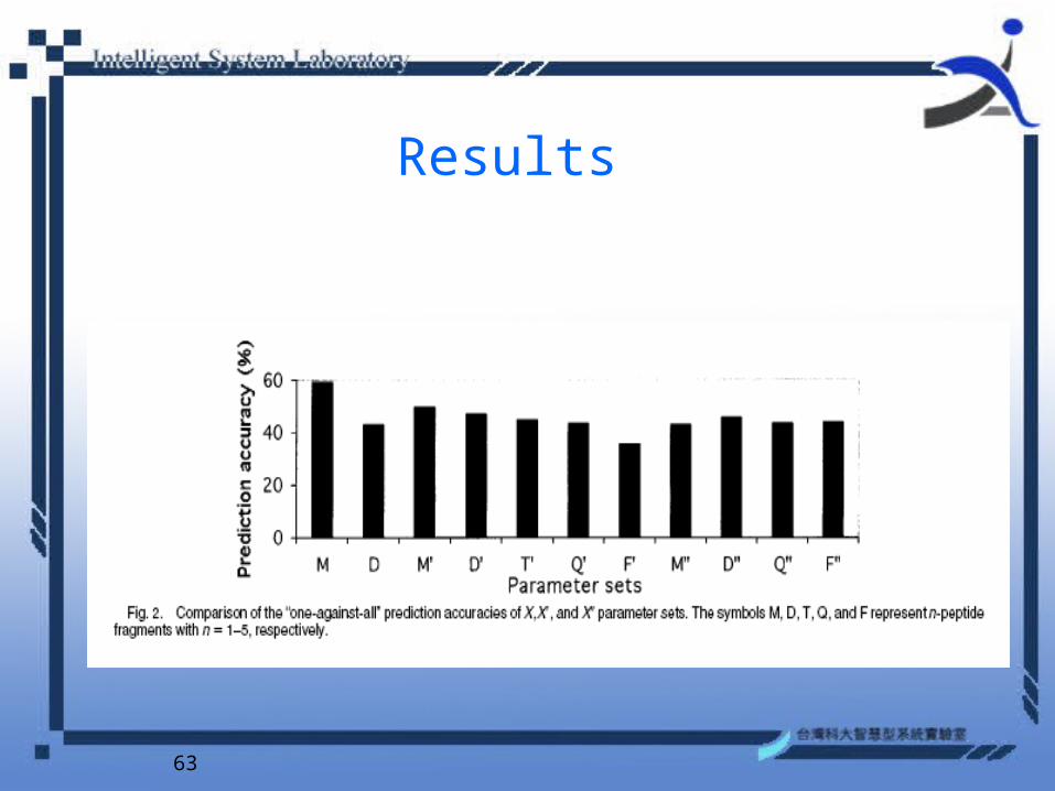
Results

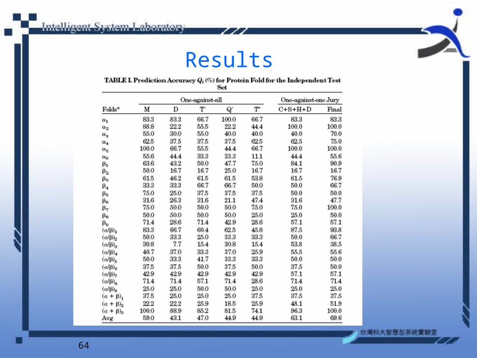
64

Results

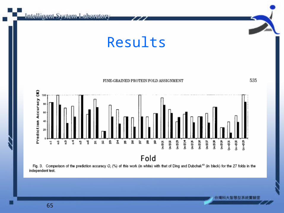
65

Results

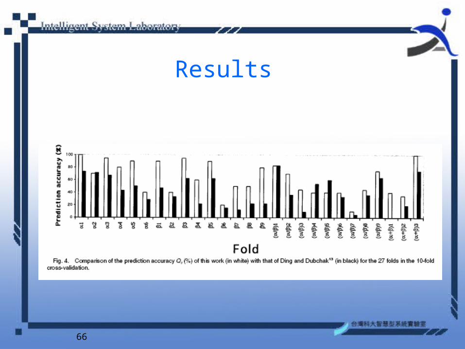
66

Results

67

Structure Example: Jury SVM Predictor

C

S

H

V

P

Z

CS

HZ

SV

CSH

VPZ

HVP

CSHV

CSHVPZ

1-VS-1

Jury (using vote)Prediction result

68

               

               

SVM

SVM

SVM

SVM

SVMcombiner

finalprediction

coding scheme 1

coding scheme 2

coding scheme 3

coding scheme 4

Structure Example:SVM Combiner

69

Thanks!