1 LOBPCG for electronic structure calculations …math.ucdenver.edu/~aknyazev/research/conf/Abinit_Householder05/... · LOBPCG for electronic structure calculations ... using the

LOBPCG for electronic structure calculations

Andrew Knyazev, CU-Denver

1

Center for Computational Mathematics, University of Colorado at Denver

Preconditioned Eigenvalue Solvers

for electronic structure calculations

Andrew V. Knyazev

Department of Mathematics and

Center for Computational Mathematics

University of Colorado at Denver

Householder Symposium XVI

May 26, 2005

Partially supported by the NSF and the LLNL



2


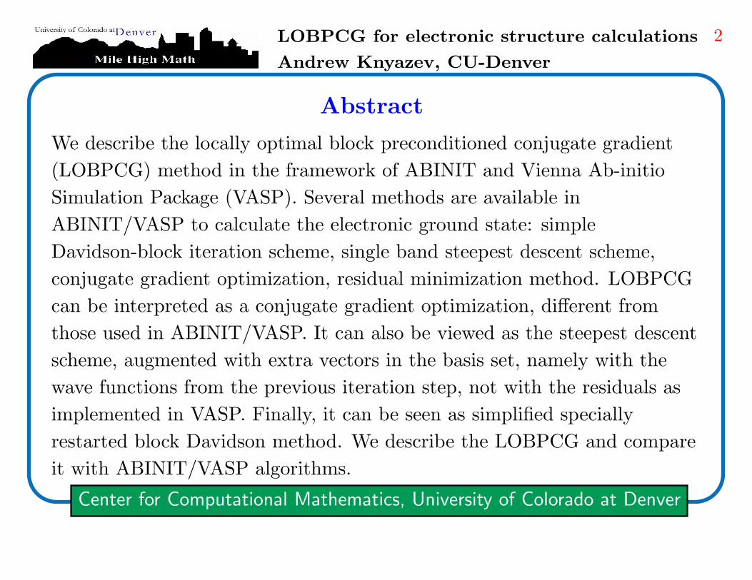
Abstract

We describe the locally optimal block preconditioned conjugate gradient

(LOBPCG) method in the framework of ABINIT and Vienna Ab-initio

Simulation Package (VASP). Several methods are available in

ABINIT/VASP to calculate the electronic ground state: simple

Davidson-block iteration scheme, single band steepest descent scheme,

conjugate gradient optimization, residual minimization method. LOBPCG

can be interpreted as a conjugate gradient optimization, different from

those used in ABINIT/VASP. It can also be viewed as the steepest descent

scheme, augmented with extra vectors in the basis set, namely with the

wave functions from the previous iteration step, not with the residuals as

implemented in VASP. Finally, it can be seen as simplified specially

restarted block Davidson method. We describe the LOBPCG and compare

it with ABINIT/VASP algorithms.



3


Acknowledgements

Partially supported by the NSF and the LLNL Center for Applied Scientific

Computing.

We would like to thank Rob Falgout, Charles Tong, Panayot Vassilevski

and other members of the Hypre Scalable Linear Solvers LLNL project

team for their support in implementing our LOBPCG eigensolver in Hypre.

John Pask and Jean-Luc Fattebert of LLNL provided invaluable help in

getting us involved in the electronic structure calculations.

LOBPCG is implemented in ABINIT rev. 4.5 and above by G. Zerah.



4



1. Electronic Structure Calculations

2. The basics of ABINIT and VASP

3. VASP band by band preconditioned steepest descent

4. ABINIT/VASP band by band preconditioned conjugate gradients

5. Locally optimal band by band preconditioned conjugate gradients

6. VASP simple block Davidson (block preconditioned steepest descent)

7. ABINIT LOBPCG

8. Conclusions



5


Electronic Structure Calculations

Quantum mechanics: a system of interacting electrons and nuclei described

by the many-body wavefunction Ψ (with MN complexity, where M is the

number of space points and N is the number of electrons), a solution to the

Schrodinger equation HΨ = EΨ, where H is the Hamiltonian operator and

E the total energy of the system. The Hamiltonian operator contains the

kinetic operators of each individual electron and nuclei and all pair-wise

Coulomb interactions. Density Functional Theory and Kohn and Sham: the

many-body Schrodinger equation can be reduced to an effective one-particle

equation:[

−∇2 + veff (r)]

ψi(r) = ǫiψi(r), which depends on the electronic

density∑N

j=1 |ψj(r)|2 (self-consistent) with N occupied and mutually

orthogonal single particle wave functions ψi, M ×N total complexity.



6


http://www.ABINIT.org/ “First-principles computation of material

properties: the ABINIT software project,” X. Gonze, J.-M. Beuken, R.

Caracas, F. Detraux, M. Fuchs, G.-M. Rignanese, L. Sindic, M. Verstraete,

G. Zerah, F. Jollet, M. Torrent, A. Roy, M. Mikami,Ph. Ghosez, J.-Y.

Raty, D.C. Allan. Computational Materials Science 25, 478-492 (2002)

http://cms.mpi.univie.ac.at/vasp/ “Efficiency of ab-initio total energy

calculations for metals and semiconductors using a plane-wave basis set,”

G. Kresse and J. Furthmuller, Comput. Mat. Sci. 6, 15-50 (1996)

http://math.cudenver.edu/˜aknyazev/ A. V. Knyazev, Toward the optimal

preconditioned eigensolver: locally optimal block preconditioned conjugate

gradient method. SIAM J. Sci. Comput. 23, no. 2, 517–541 (2001)



7


The basics of ABINIT and VASP

ABINIT and Vienna Ab-initio Simulation Package (VASP) are complex

packages for performing ab-initio quantum-mechanical molecular dynamics

simulations using a plane wave (PW) basis set. Generally not more than

100 PW per atom are required to describe bulk materials, in most cases

even 50 PW per atom will be sufficient for a reliable description.

Multiplication by the Hamiltonian in the plain wave basis involves both

Fourier (for the Laplacian) and real (for the potential)l spaces, thus DFFT

is called twice per multiplication. Since the Laplacian becomes diagonal in

the Fourier space, diagonal preconditioning is useful.

Alternatively, real-space FEM and finite difference codes are available, e.g.,

Multigrid Instead of the K-spAce (MIKA). In real space approximations

the number of basis functions is 10-100 times larger than that with plain

waves, and sophisticated preconditioning (usually multigrid) is necessary.



8


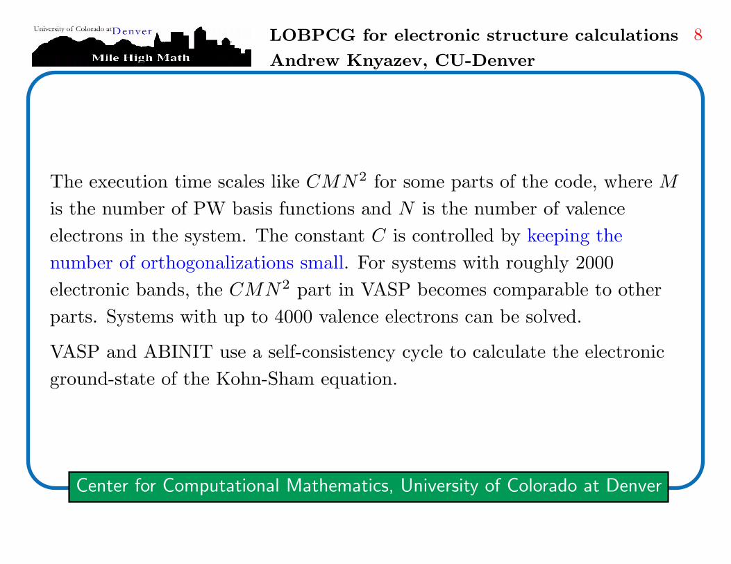
The execution time scales like CMN2 for some parts of the code, where M

is the number of PW basis functions and N is the number of valence

electrons in the system. The constant C is controlled by keeping the

number of orthogonalizations small. For systems with roughly 2000

electronic bands, the CMN2 part in VASP becomes comparable to other

parts. Systems with up to 4000 valence electrons can be solved.

VASP and ABINIT use a self-consistency cycle to calculate the electronic

ground-state of the Kohn-Sham equation.



9


The Kohn-Sham (KS) eigenvalue problem (eigenproblem) to solve is

H|φn〉 = ǫnS|φn〉, n = 1, . . . , Nb,

where H is the Kohn-Sham Hamiltonian, |φn〉 is the band eigenstate wave

function, ǫn is the eigenvalue, describing the band energy, and S is the

overlap matrix, specifying the orthonormality constraints of eigenstates for

different bands. In PW basis, the calculations of H|φn〉 and S|φn〉 are

relatively inexpensive. Matrices H and S are Hermitian and S is positive

definite. In VASP, S is not identity because of the use of ultra-soft pseudo

potentials. Nb ≪ N wavefunctions of occupied orbitals are computed. In a

self-consistent calculation, optimization of the charge density, appearing in

the Hamiltonian, and wavefunctions |φn〉 of the KS eigenproblem is done in

a cycle. In this talk, we consider only the KS eigenproblem numerical

solution part, not the charge density updates.



10


The expectation value of the Hamiltonian for a wavefunction |φapp〉

ǫapp =〈φapp|H|φapp〉

〈φapp|S|φapp〉

is called the Rayleigh quotient. Variation of the Rayleigh quotient with

respect to 〈φapp| leads to the residual vector defined as

|R(|φapp〉)〉 = (H − ǫappS)|φapp〉.

To accelerate the convergence, a preconditioner K is applied to the residual:

|p(|φapp〉)〉 = K|R(|φapp〉)〉 = K(H − ǫappS)|φapp〉.

The preconditioner K is Hermitian, often simply an inverse to the main

diagonal of H − ǫappS or of H - the latter is used in our tests for this talk.



11


Another core technique used in VASP is the Rayleigh-Ritz variational

scheme in a subspace spanned by Na wavefunctions |φi〉, i = 1, . . . , Na:

〈φj |H|φi〉 = Hij , 〈φj |S|φi〉 = Sij , HijUjk = ǫkSijUjk, |φj〉 = Ujk|φk〉,

using the standard summation agreement on repeated indexes from 1 to

Na. Here, on the first two steps we compute the Na-by-Na Gram matrices

of the KS quadratic forms with respect to the given basis of wavefunctions.

Then we solve a matrix generalized eigenproblem with the Gram matrices

to compute the Ritz values ǫk. Finally, we calculate the Ritz functions |φj〉.

The set of wavefunctions here is not assumed to be S-orthonormal and may

include the approximate KS eigenfunctions as well as preconditioned

residuals and other functions.



12


VASP single band preconditioned steepest descent

The method is robust and simple. It utilizes the two-term recurrence

|φ(M+1)〉 ∈ Span {|p(M)〉, |φ(M)〉},

where |p(M)〉 = |p(|φ(M)〉})〉 is the preconditioned residual on the M -th

iteration and |φ(M+1)〉 is chosen to minimize the Rayleigh quotient ǫ(M+1)

by using the Rayleigh–Ritz method on this two dimensional subspace. It

can only compute approximately the lowest eigenstate |φ1〉. The

asymptotic convergence speed is determined, when the preconditioner K is

positive definite, by the ratio κ of the largest and the smallest positive

eigenvalues of K(H − ǫ1S).

Two-term recurrence + Rayleigh–Ritz method =

Singe Band Steepest Descent Method



13


100 200 300 400 500 600 700 800 900 1000

10−3

10−2

10−1

100

101

102

VASP single band steepest descent

Ab

so

lute

eig

en

va

lue

err

ors

Iteration number2 4 6 8 10 12

10−10

10−8

10−6

10−4

10−2

100

102


Ab

so

lute

eig

en

va

lue

err

ors

Iteration number

Figure 1: SD κ ≈ 4 ∗ 102 (left) and with diagonal preconditioning κ ≈ 2 (right),

no cluster of eigenvalues in these tests



14


100 200 300 400 500 600 700 800 900 1000

10−2

10−1

100

101

102


Ab

so

lute

eig

en

va

lue

err

ors

Iteration number100 200 300 400 500 600 700 800 900 1000

10−4

10−3

10−2

10−1

100

101

102


Ab

so

lute

eig

en

va

lue

err

ors

Iteration number

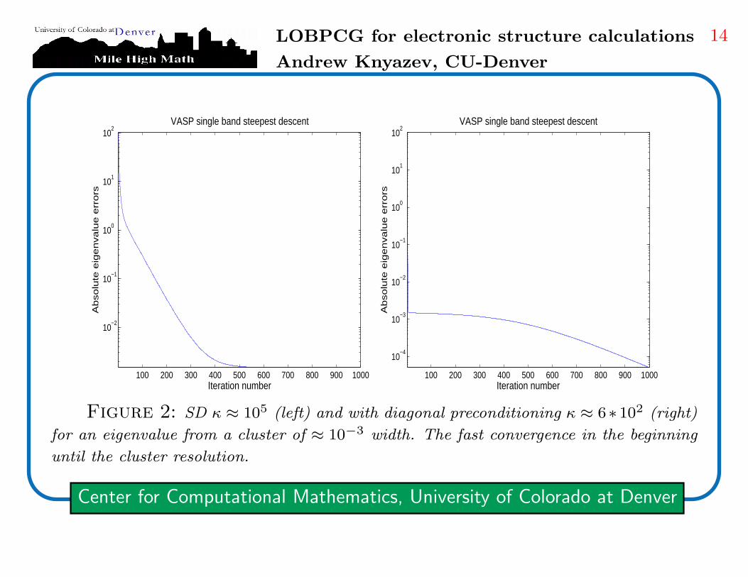
Figure 2: SD κ ≈ 105 (left) and with diagonal preconditioning κ ≈ 6∗10

2 (right)

for an eigenvalue from a cluster of ≈ 10−3 width. The fast convergence in the beginning

until the cluster resolution.



15


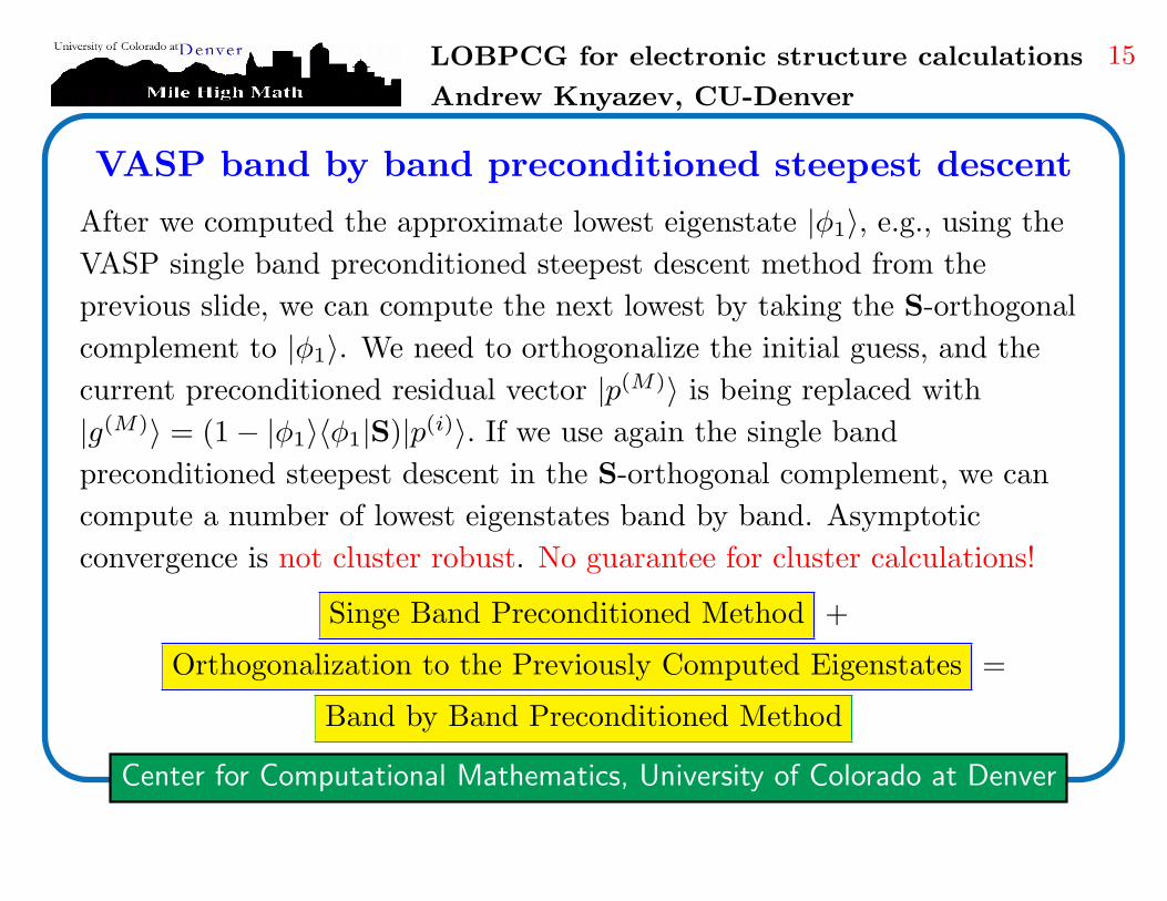
VASP band by band preconditioned steepest descent

After we computed the approximate lowest eigenstate |φ1〉, e.g., using the

VASP single band preconditioned steepest descent method from the

previous slide, we can compute the next lowest by taking the S-orthogonal

complement to |φ1〉. We need to orthogonalize the initial guess, and the

current preconditioned residual vector |p(M)〉 is being replaced with

|g(M)〉 = (1 − |φ1〉〈φ1|S)|p(i)〉. If we use again the single band

preconditioned steepest descent in the S-orthogonal complement, we can

compute a number of lowest eigenstates band by band. Asymptotic

convergence is not cluster robust. No guarantee for cluster calculations!

Singe Band Preconditioned Method +

Orthogonalization to the Previously Computed Eigenstates =

Band by Band Preconditioned Method



16


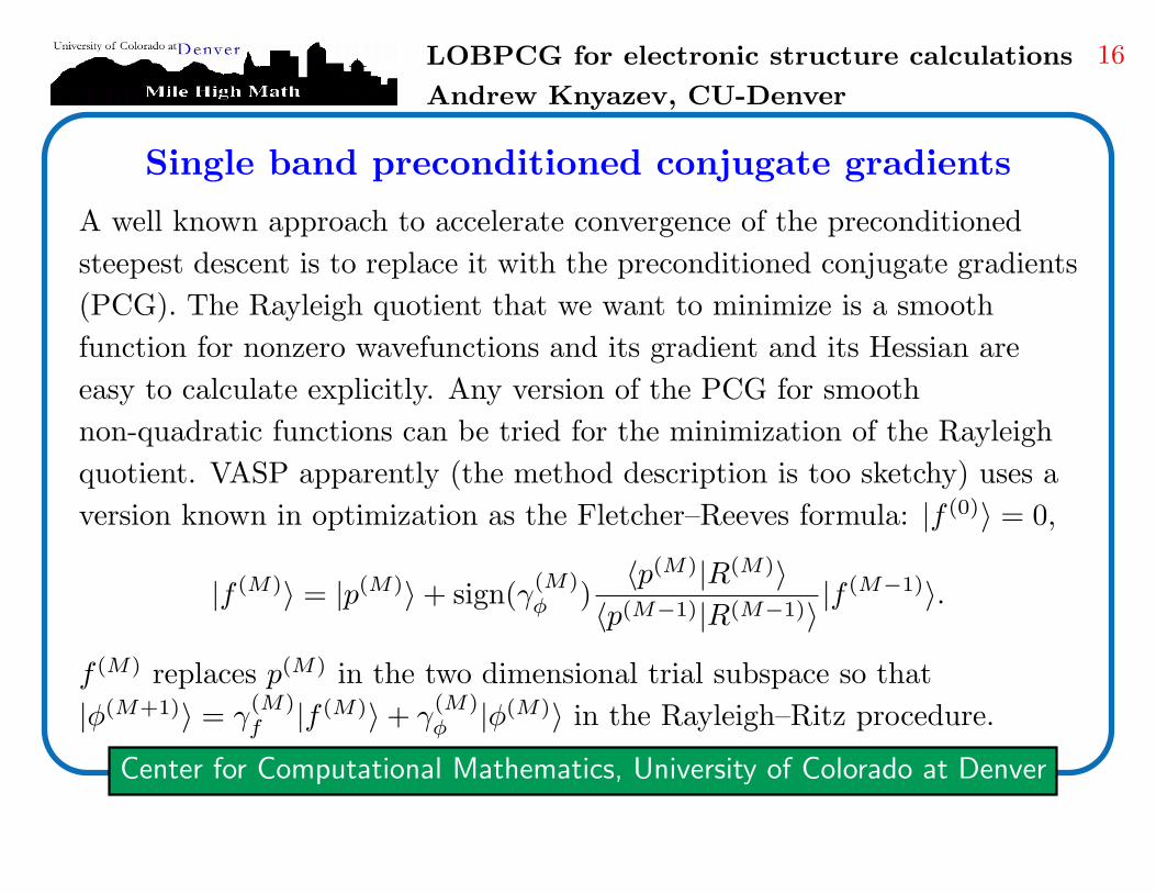
Single band preconditioned conjugate gradients

A well known approach to accelerate convergence of the preconditioned

steepest descent is to replace it with the preconditioned conjugate gradients

(PCG). The Rayleigh quotient that we want to minimize is a smooth

function for nonzero wavefunctions and its gradient and its Hessian are

easy to calculate explicitly. Any version of the PCG for smooth

non-quadratic functions can be tried for the minimization of the Rayleigh

quotient. VASP apparently (the method description is too sketchy) uses a

version known in optimization as the Fletcher–Reeves formula: |f (0)〉 = 0,

|f (M)〉 = |p(M)〉 + sign(γ(M)φ )

〈p(M)|R(M)〉

〈p(M−1)|R(M−1)〉|f (M−1)〉.

f (M) replaces p(M) in the two dimensional trial subspace so that

|φ(M+1)〉 = γ(M)f |f (M)〉 + γ

(M)φ |φ(M)〉 in the Rayleigh–Ritz procedure.



17


Band by band preconditioned conjugate gradients


single band preconditioned conjugate gradients method from the previous

slide, we can compute the next lowest by taking the S-orthogonal

complement to |φ1〉. We need to orthogonalize the initial guess, and the

current preconditioned residual vector |p(M)〉 is being replaced with

|g(M)〉 = (1 − |φ1〉〈φ1|S)|p(i)〉. Fletcher–Reeves formula changes to:

|f (M)〉 = |g(M)〉 + sign(γ(M)φ )

〈g(M)|R(M)〉

〈g(M−1)|R(M−1)〉|f (M−1)〉, |f (0)〉 = 0.

and |φ(M+1)〉 = γ(M)f |f (M)〉 + γ

(M)φ |φ(M)〉 in the Rayleigh–Ritz procedure.



18


100 200 300 400 500 600 700 800 900 1000

10−6

10−4

10−2

100

102


Abs

olut

e ei

genv

alue

err

ors

Iteration number5 10 15 20 25

10−10

10−8

10−6

10−4

10−2

100

102


Abso

lute

eig

enva

lue

erro

rs

Iteration number

20 40 60 80 100 120

10−10

10−8

10−6

10−4

10−2

100

102

VASP single band CG

Abso

lute

eig

enva

lue

erro

rs

Iteration number2 4 6 8 10 12 14

10−10

10−8

10−6

10−4

10−2

100

102

VASP single band CG

Abso

lute

eig

enva

lue

erro

rs

Iteration number

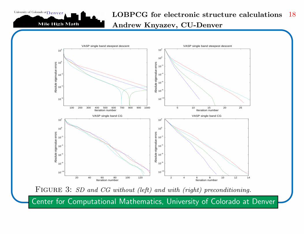
Figure 3: SD and CG without (left) and with (right) preconditioning.



19


Locally optimal single band PCG

The method combines robustness and simplicity of the preconditioned

steepest descent method with a three-term recurrence formula:

|φ(M+1)〉 ∈ Span {|p(M)〉, |φ(M)〉, |φ(M−1)〉},

where |p(M)〉 = |p(|φ(M)〉)〉 is the preconditioned residual on the M -th

iteration and |φ(M+1)〉 is chosen to minimize the Rayleigh quotient ǫ(M+1)

by using the Rayleigh–Ritz method on this three dimensional subspace. The

asymptotic convergence speed to lowest eigenstate |φ1〉 depends, when the

preconditioner K is positive definite, on the square root of the ratio κ of the

largest and the smallest positive eigenvalues of K(H − ǫ1S).

Three-term recurrence + Rayleigh–Ritz method =

Locally Optimal Conjugate Gradient Method



20


Locally optimal band by band PCG


locally optimal single band preconditioned conjugate gradients method

from the previous slide, we can compute the next lowest by taking the

S-orthogonal complement to |φ1〉. We need to orthogonalize the initial

guess, and the current preconditioned residual vector |p(M)〉 is being

replaced with |g(M)〉 = (1 − |φ1〉〈φ1|S)|p(i)〉. No other changes are needed.

The band by band implementation of the locally optimal PCG method

shares the same advantages and difficulties with other band by band

iterative schemes, such as low memory requirements and troubles resolving

clusters of eigenvalues.



21


Locally optimal vs. Fletcher–Reeves PCG

The methods converge quite similarly in practice in many cases, though a

theoretical explanation of this fact is still not available. The costs per

iterations are also similar, but the locally optimal method is slightly more

expensive. There is known (Knyazev, 2001) a reasonably stable

implementation of the locally optimal method that uses an implicitly

computed linear combination of |φ(M)〉, |φ(M−1)〉 instead |φ(M−1)〉 in the

Rayleigh-Ritz procedure. The convergence of the locally optimal method is

well supported theoretically, while the convergence of the Fletcher–Reeves

version is not.

Perhaps, the main practical advantage of the locally optimal method is

that it allows a straightforward block generalization to calculate several

eigenpairs simultaneously.



22


Block eigenvalue iterations

A well known idea of using Simultaneous, or Block Iterations provides an

important improvement over single-vector methods, and permits us to

compute an invariant subspace, rather than one eigenvector at a time,

which allows robust calculations of clustered eigenvalues and corresponding

invariant subspaces. It can also serve as an acceleration technique over a

single-vector methods on parallel computers, as convergence for extreme

eigenvalues usually increases with the size of the block, and every step can

be naturally implemented on wide varieties of multiprocessor computers as

well as to take advantage processors cache through the use of high level

BLAS libraries.



23


VASP simple block Davidson(Block preconditioned steepest descent)

|φ(M+1)i 〉 ∈ Span {|p

(M)1 〉, . . . , |p

(M)Nb

〉, |φ(M)1 〉, . . . , |φ

(M)Nb

〉}, i = 1, . . . , Nb,

where |p(M)i 〉 = |p(|φ(M)〉)〉 is the preconditioned residual on the M -th

iteration for the ith band and |φ(M+1)i 〉 are chosen as Ritz functions by

using the Rayleigh–Ritz method on this 2Nb dimensional subspace, to

approximate the Nb lowest exact KS eigenstates |φi〉. The asymptotic

convergence speed for the ith band is determined, when the preconditioner

K is positive definite, by the ratio κi of the largest and the smallest

positive eigenvalues of K(H − ǫiS).

Trial subspace of all approx. eigenfunctions and residuals +

Rayleigh–Ritz method = Block Steepest Descent Method



24


100 200 300 400 500 600 700 800 900 1000

10−6

10−4

10−2

100

102


Abs

olut

e ei

genv

alue

err

ors


10−10

10−8

10−6

10−4

10−2

100

102


Abso

lute

eig

enva

lue

erro

rs

Iteration number

100 200 300 400 500 600 700 800 900 1000

10−15

10−10

10−5

100

VASP simple block Davidson

Eig

enva

lue

erro

rs

Iteration number5 10 15 20 25 30 35 40

10−10

10−5

100


Eige

nval

ue e

rrors

Iteration number

Figure 4: SD and block SD without (left) and with (right) preconditioning.



25


100 200 300 400 500 600 700 800 900 100010

−5

10−4

10−3

10−2

10−1

100

101


Abs

olut

e ei

genv

alue

err

ors


10−6

10−4

10−2

100


Abs

olut

e ei

genv

alue

err

ors

Iteration number

100 200 300 400 500

10−15

10−10

10−5

100


Eige

nval

ue e

rrors

Iteration number2 4 6 8 10 12 14 16 18

10−10

10−5

100


Eige

nval

ue e

rrors

Iteration number

Figure 5: SD and block SD without (left) and with (right) preconditioning.



26


General block Davidson with a trivial restart

The block preconditioned steepest descent is the simplest case of a general

block Davidson method. In the general block Davidson method, the trial

subspace of the Rayleigh–Ritz method increases in each step by Nb current

preconditioned residuals, i.e., in its original formulation the general block

Davidson method memory requirements grow with every iteration by Nb

vectors. Such method converges faster than the block steepest descent, but

the costs are growing with the number of iterations.

A restart is needed in practice. A trivial restart at every step restricts the

trial subspace only to the Nb approximate eigenfunctions and one set of Nb

preconditioned residuals, thus, leading to the block preconditioned steepest

descent from the previous slide, utilized in VASP.



27


General block Davidson with a non-standard restart

A non-standard restart in the block Davidson method is suggested in

C. Murray, S. C. Racine, E. R. Davidson, Improved algorithms for the

lowest few eigenvalues and associated eigenvectors of large matrices. J.

Comput. Phys. 103 (1992), no. 2, 382–389.

A. V. Knyazev, Toward the optimal preconditioned eigensolver: locally

optimal block preconditioned conjugate gradient method. SIAM J. Sci.

Comput. 23 (2001), no. 2, 517–541 (electronic).

In addition to the usual Nb current approximate eigenfunctions

|φ(M)1 〉, . . . , |φ

(M)Nb

〉, we also add Nb approximate eigenfunctions from the

previous step: |φ(M−1)1 〉, . . . , |φ

(M−1)Nb

〉.



28


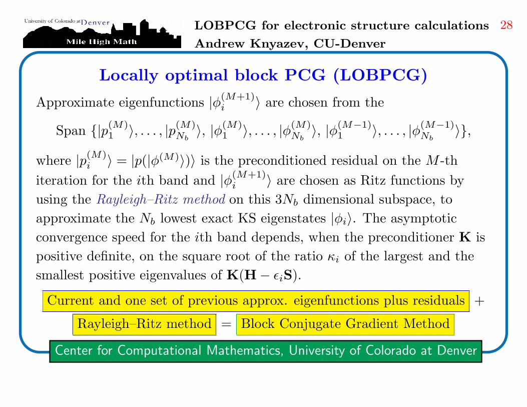
Locally optimal block PCG (LOBPCG)

Approximate eigenfunctions |φ(M+1)i 〉 are chosen from the

Span {|p(M)1 〉, . . . , |p

(M)Nb

〉, |φ(M)1 〉, . . . , |φ

(M)Nb

〉, |φ(M−1)1 〉, . . . , |φ

(M−1)Nb

〉},

where |p(M)i 〉 = |p(|φ(M)〉)〉 is the preconditioned residual on the M -th

iteration for the ith band and |φ(M+1)i 〉 are chosen as Ritz functions by

using the Rayleigh–Ritz method on this 3Nb dimensional subspace, to

approximate the Nb lowest exact KS eigenstates |φi〉. The asymptotic

convergence speed for the ith band depends, when the preconditioner K is

positive definite, on the square root of the ratio κi of the largest and the

smallest positive eigenvalues of K(H − ǫiS).

Current and one set of previous approx. eigenfunctions plus residuals +

Rayleigh–Ritz method = Block Conjugate Gradient Method



29


LOBPCG interpretations:

• LOBPCG can be interpreted as a specific version of conjugate gradient

optimization, different from those used in VASP, that can be easily

applied in the block form.

• It can also be viewed as the block steepest descent scheme, augmented

with extra vectors in the basis set, namely with the wavefunctions from

the previous iteration step, not with the residuals as in the block

Davidson method.

• Finally, it can be seen as simplified specially restarted block Davidson

method. It seems to preserve the fast convergence of the block

Davidson at the much lower costs.



30


20 40 60 80 100 120 140

10−10

10−8

10−6

10−4

10−2

100

102

VASP single band CG

Abso

lute

eig

enva

lue

erro

rs

Iteration number10 20 30 40 50 60 70

10−10

10−8

10−6

10−4

10−2

100

102

VASP single band CG

Abso

lute

eig

enva

lue

erro

rs

Iteration number

10 20 30 40 50 60 70 80 90

10−10

10−5

100

LO Block CG

Eige

nval

ue e

rrors


10−10

10−5

100

LO Block CG

Eige

nval

ue e

rrors

Iteration number

Figure 6: CG and block CG without (left) and with (right) preconditioning.



31


50 100 150 200

10−8

10−6

10−4

10−2

100

VASP single band CG

Abso

lute

eig

enva

lue

erro

rs

Iteration number20 40 60 80 100 120 140 160 180

10−8

10−6

10−4

10−2

100

VASP single band CG

Abso

lute

eig

enva

lue

erro

rs

Iteration number

10 20 30 40 50 60

10−10

10−8

10−6

10−4

10−2

100

LO Block CG

Eige

nval

ue e

rrors

Iteration number2 4 6 8 10 12

10−12

10−10

10−8

10−6

10−4

10−2

100

LO Block CG

Eige

nval

ue e

rrors

Iteration number

Figure 7: CG and block CG without (left) and with (right) preconditioning.



32


Implementing LOBPCG in ABINIT

ABINIT is a FORTRAN 90 parallel code with timing. ABINIT rev. 4.5

manual: “The algorithm LOBPCG is available as an alternative to

band-by-band conjugate gradient, from Gilles Zerah. Use wfoptalg=4 . See

Test v4 No. 93 and 94. The band-by-band parallelization of this algorithm

should be much better than the one of the usual algorithm.” The

implementation follows my MATLAB code of LOBPCG rev. 4.10 with

some simplifications.



33


Testing LOBPCG in ABINIT

Test example results provided by G. Zerah: 32 boron atoms and 88 bands,

nonselfconsistent. Band-by-band PCG every band converges in 4-6

iterations. LOBPCG block size 88 converges in 2-4 iterations,

approximately 2 times faster. LOBPCG block size 20 with partial

convergence converges (we do not wait for the previous block to converge to

compute the next, by limiting the number of LOBPCG iteration to

nline=4) is surprisingly even faster. We can even limit nline=2 and get the

same overall complexity as for nline=4.

Mixed results for LOBPCG II applied to the selfconsistent calculation of

Hydrogen and nonselfconsistent 32 boron atoms: slow convergence for some

bands.



34


LOBPCG in PETSCAN

Work by others on LOBPCG in material sciences:

“Comparison of Nonlinear Conjugate-Gradient Methods for Computing the

Electronic Properties of Nanostructure Architectures,” Stanimire Tomov,

Julien Langou, Andrew Canning, Lin-Wang Wang, and Jack Dongarra

implement and test LOBPCG in PESCAN, where a semi-empirical

potential or a charge patching method is used to construct the potential

and only the eigenstates of interest around a given energy are calculated

using folded spectrum: “if memory is not a problem and block version of

the matrix-vector multiplication can be efficiently implemented, the

FS-LOBPCG will be the method of choice for the type of problems

discussed.”



35


Conclusions

• LOBPCG is a valuable alternative to eigensolvers currently used in

electronic structure calculations

• Initial numerical results look promising, but more testing is needed on

larger problems

Future work

• ABINIT LOBPCG testing vs. the default CG solver

• New LOBPCG modifications with reduced orthogonalization costs

• Revisiting traditional preconditioning

• Collaboration with John Pask of LLNL on implementing LOBPCG in

the in-house FEM electronic structure calculations code

Documents

1 LOBPCG for electronic structure calculations …math.ucdenver.edu/~aknyazev/research/conf/Abinit_Householder05/... · LOBPCG for electronic structure calculations ... using the