Embed Size (px)
Citation preview

2
Linear ProgrammingWhat is it?
Quintessential tool for optimal allocation of scarce resources, among a number of competing activities. (e.g., see ORF 307) Powerful and general problem-solving method.
shortest path, max flow, min cost flow, generalized flow, multicommodity flow, MST, matching, 2-person zero sum games
Why significant? Fast commercial solvers: CPLEX, OSL, Lindo. Powerful modeling languages: AMPL, GAMS. Ranked among most important scientific advances of 20th century. Also a general tool for attacking NP-hard optimization problems. Dominates world of industry.
ex: Delta claims saving $100 million per year using LP
3
Example
1 2
1 2
1 2
1 2
1 2
max
4 8
2 10
5 2 2
, 0
x x
Subject to
x x
x x
x x
x x
4
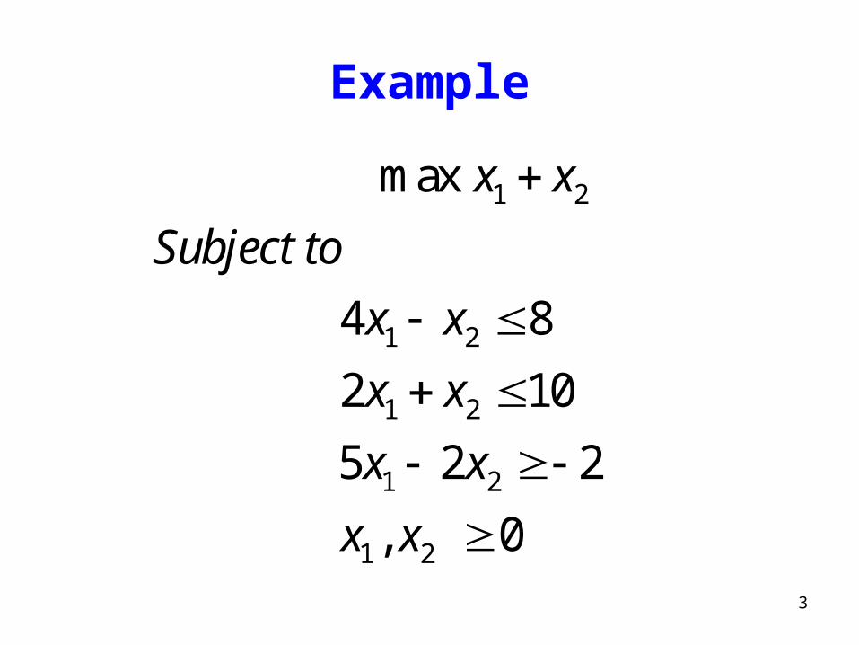
Geometry Observation. Regardless of objective function (convex) coefficients, an optimal solution occurs at an extreme point.
5
Standard and slack forms
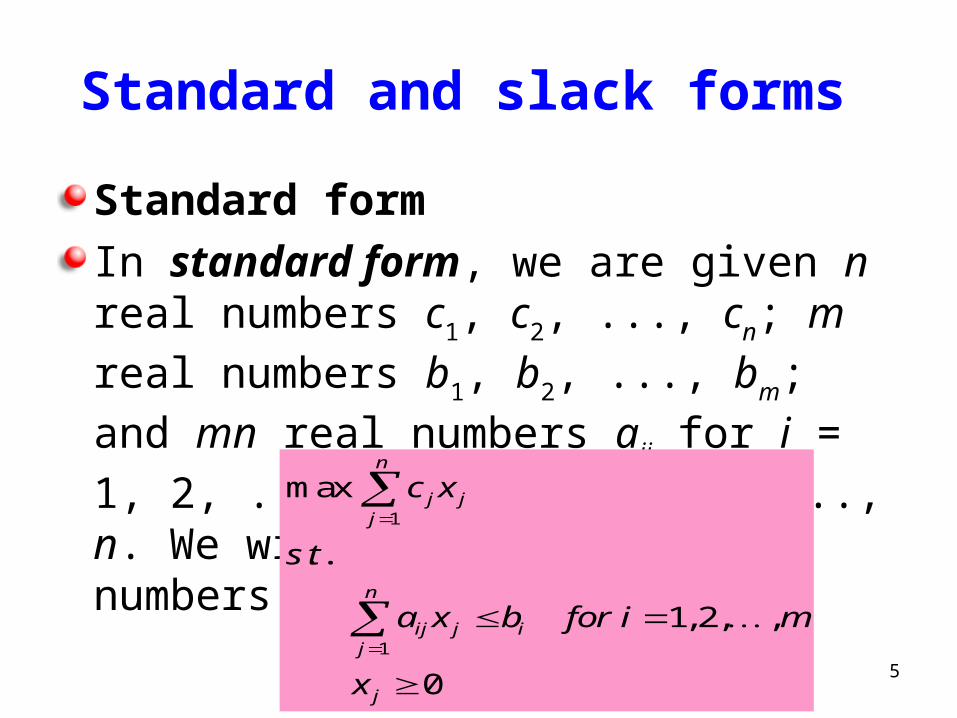
Standard form
In standard form, we are given n real numbers c1, c2, ..., cn; m real numbers b1, b2, ..., bm; and
mn real numbers aij for i = 1, 2, ..., m and j = 1,
2, ..., n. We wish to find n real numbers x1,
x2, ..., xn that1
1
max
. .
1,2, ,
0
n
j jj
n
ij j ij
j
c x
s t
a x b for i m
x

6
Standard and slack forms
Standard form
In standard form, we are given n real numbers c1, c2, ..., cn; m real numbers b1, b2, ..., bm; and
mn real numbers aij for i = 1, 2, ..., m and j = 1,
2, ..., n. We wish to find n real numbers x1,
x2, ..., xn that max
. .
0
TC X
s t
AX b
X
7
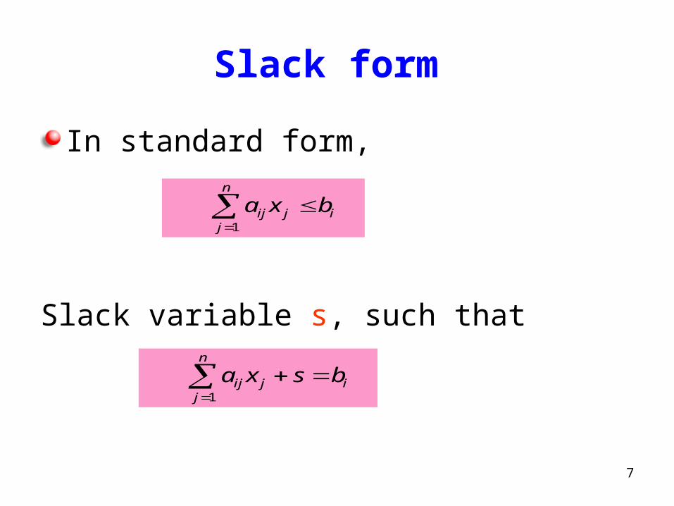
Slack form
In standard form,
Slack variable s, such that
1
n
ij j ij
a x b
1
n
ij j ij
a x s b
8
The simplex algorithm
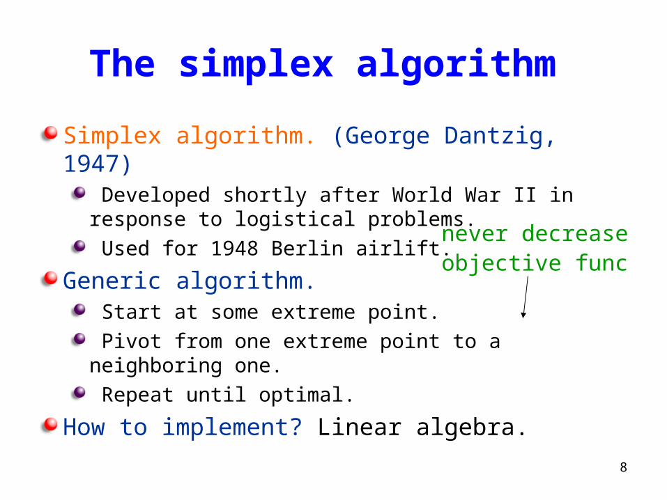
Simplex algorithm. (George Dantzig, 1947) Developed shortly after World War II in response to logistical problems. Used for 1948 Berlin airlift.
Generic algorithm. Start at some extreme point. Pivot from one extreme point to a neighboring one. Repeat until optimal.
How to implement? Linear algebra.
never decrease objective func
9
Illustration of Simplex
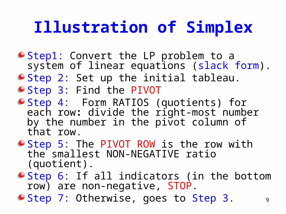
Step1: Convert the LP problem to a system of linear equations (slack form). Step 2: Set up the initial tableau. Step 3: Find the PIVOT Step 4: Form RATIOS (quotients) for each row: divide the right-most number by the number in the pivot column of that row. Step 5: The PIVOT ROW is the row with the smallest NON-NEGATIVE ratio (quotient).Step 6: If all indicators (in the bottom row) are non-negative, STOP. Step 7: Otherwise, goes to Step 3.
10
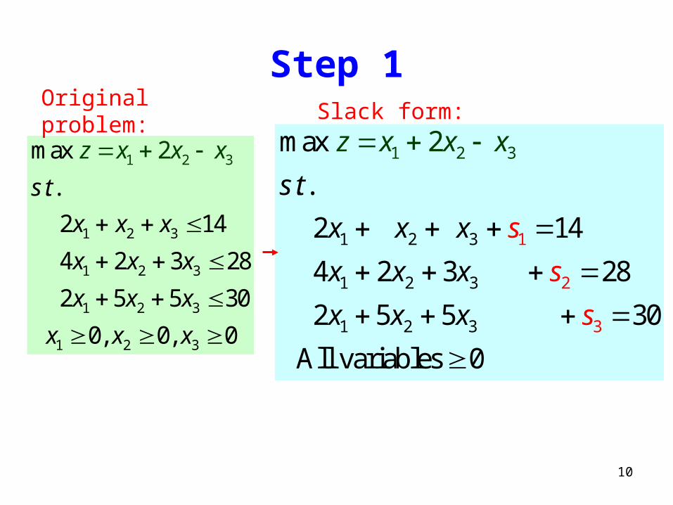
Step 1
1 2 3
1 2 3
1 2 3
1 2 3
1 2 3
max
. .
2 14
4 2 3 28
2 5 5 30
0, 0 0
2
,
s t
x x x
x x x
x x x
x x
z x x
x
x
Original problem:
1 2 3
1 2 3
1 2 3
1 2
2
3
3
1
max
. .
2 14
4 2 3 28
2 5 5 30
All variab
2
les 0
s t
x x x
x x x
s
s
s
x
x x
z
x
x x
Slack form:
11
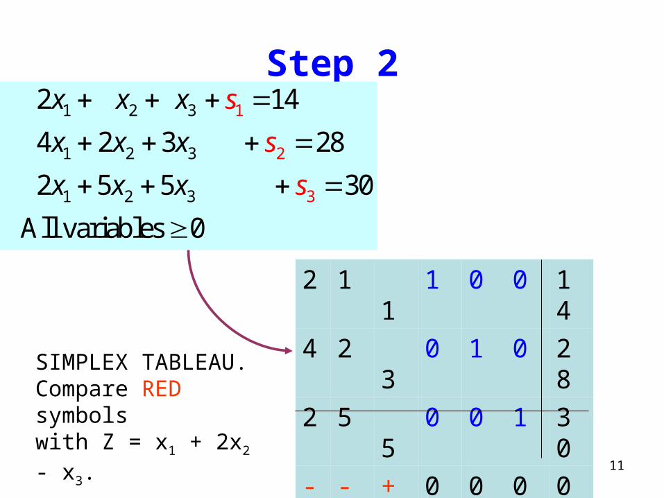
Step 21 2 3
1 2
1
23
1 3 32
2 14
4 2 3 28
2 5 5 30
All variables 0
x x x
x x x
x x x
s
s
s
2 1 1 1 0 0 14
4 2 3 0 1 0 28
2 5 5 0 0 1 30
-1 -2 +1 0 0 0 0
SIMPLEX TABLEAU.Compare RED symbolswith Z = x1 + 2x2 - x3.
12
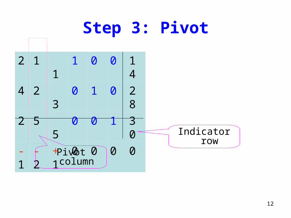
Step 3: Pivot
2 1 1 1 0 0 14
4 2 3 0 1 0 28
2 5 5 0 0 1 30
-1 -2 +1 0 0 0 0
Pivot column
Indicator row
13
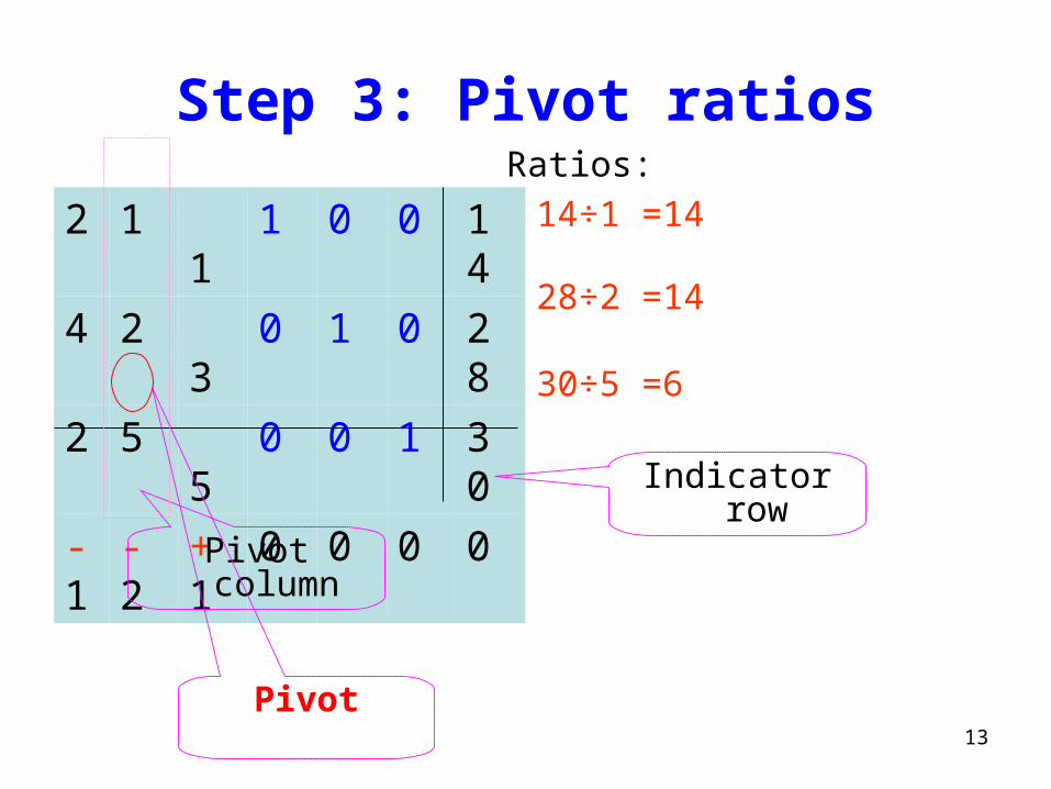
Step 3: Pivot ratios
2 1 1 1 0 0 14
4 2 3 0 1 0 28
2 5 5 0 0 1 30
-1 -2 +1 0 0 0 0
Pivot column
Indicator row
Ratios:
14÷1 =14
28÷2 =14
30÷5 =6
Pivot

14
Step 4: entering variable
2 1 1 1 0 0 14
4 2 3 0 1 0 28
2 5 5 0 0 1 30
-1 -2 +1 0 0 0 0
r1:
r2:
r3:
r4: 2 1 1 1 0 0 14
4 2 3 0 1 0 28
2/5 1 1 0 0 1/5 6
-1 -2 +1 0 0 0 0
R3=(r3 /5)

15
Step 4: leaving variable
r1:
r2:
R3:
r4:
2 1 1 1 0 0 14
4 2 3 0 1 0 28
2/5 1 1 0 0 1/5 6
-1 -2 +1 0 0 0 0
R1=r1 - R3
R2=r2-2R3
R4=r4+2R3
8/5 0 0 1 0 -1/5 8
16/5 0 1 0 1 -2/5 16
2/5 1 1 0 0 1/5 6
-1/5 0 3 0 0 2/5 12
R1:
R2:
R3:
R4:
16
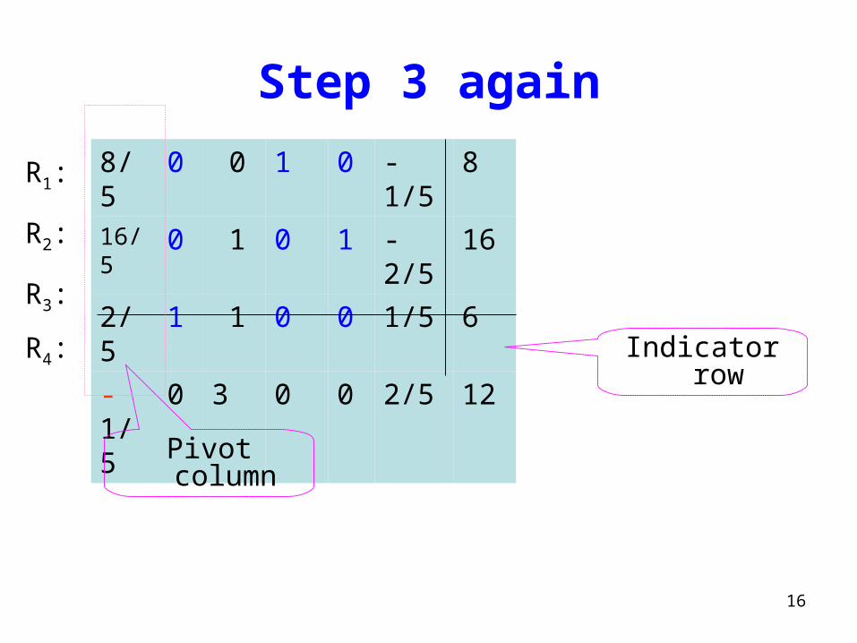
Step 3 again
8/5 0 0 1 0 -1/5 8
16/5 0 1 0 1 -2/5 16
2/5 1 1 0 0 1/5 6
-1/5 0 3 0 0 2/5 12
R1:
R2:
R3:
R4:
Pivot column
Indicator row
17
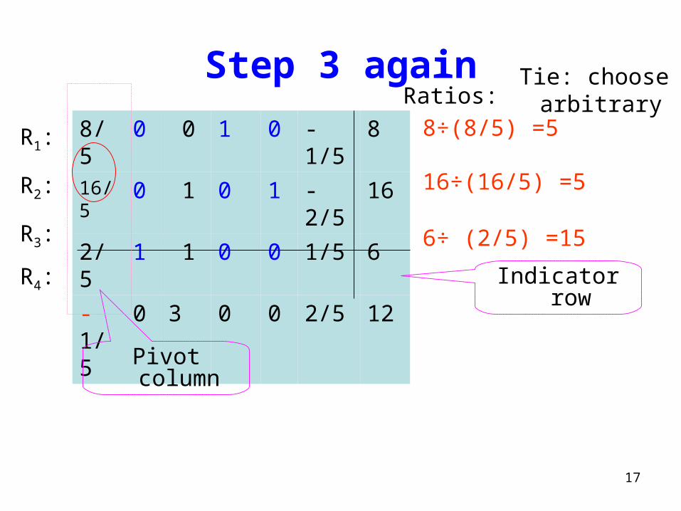
Step 3 again
8/5 0 0 1 0 -1/5 8
16/5 0 1 0 1 -2/5 16
2/5 1 1 0 0 1/5 6
-1/5 0 3 0 0 2/5 12
R1:
R2:
R3:
R4:
Pivot column
Indicator row
Ratios:
8÷(8/5) =5
16÷(16/5) =5
6÷ (2/5) =15
Tie: choose arbitrary
18
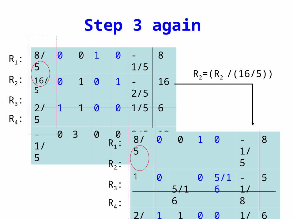
Step 3 again
8/5 0 0 1 0 -1/5 8
16/5 0 1 0 1 -2/5 16
2/5 1 1 0 0 1/5 6
-1/5 0 3 0 0 2/5 12
R1:
R2:
R3:
R4:
8/5 0 0 1 0 -1/5 8
1 0 5/16 0 5/16 -1/8 5
2/5 1 1 0 0 1/5 6
-1/5 0 3 0 0 2/5 12
R1:
R2:
R3:
R4:
R2=(R2 /(16/5))
19
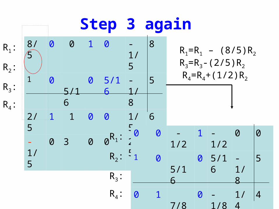
Step 3 again8/5 0 0 1 0 -1/5 8
1 0 5/16 0 5/16 -1/8 5
2/5 1 1 0 0 1/5 6
-1/5 0 3 0 0 2/5 12
R1:
R2:
R3:
R4:
0 0 -1/2 1 -1/2 0 0
1 0 5/16 0 5/16 -1/8 5
0 1 7/8 0 -1/8 1/4 4
0 0 49/16 0 1/16 3/8 13
R1:
R2:
R3:
R4:
R1=R1 – (8/5)R2
R3=R3-(2/5)R2
R4=R4+(1/2)R2

20
STOP
0 0 -1/2 1 -1/2 0 0
1 0 5/16 0 5/16 -1/8 5
0 1 7/8 0 -1/8 1/4 4
0 0 49/16 0 1/16 3/8 13
R1:
R2:
R3:
R4:
x1 x2 x3 s1 s2 s3
x3=s2=s3=0
x1=5, x2=4, s1=0
z =13
Finally, the optimal solution of LP is
21
History of LP
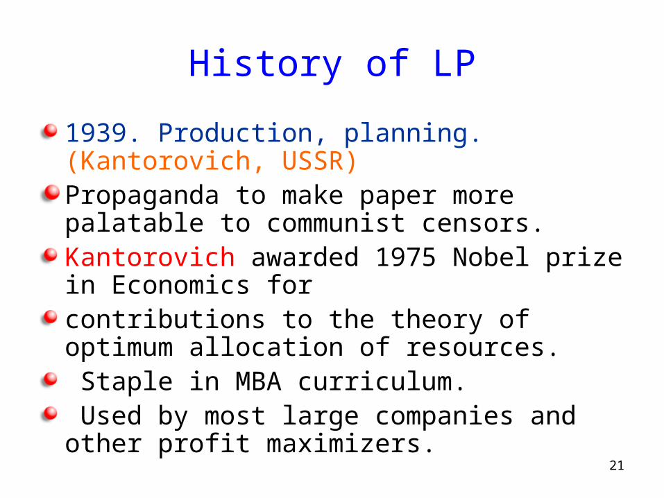
1939. Production, planning. (Kantorovich, USSR)Propaganda to make paper more palatable to communist censors.Kantorovich awarded 1975 Nobel prize in Economics forcontributions to the theory of optimum allocation of resources. Staple in MBA curriculum. Used by most large companies and other profit maximizers.
22
History
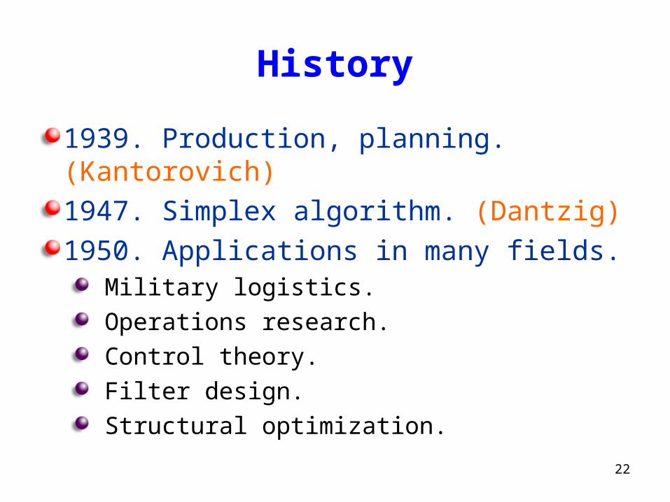
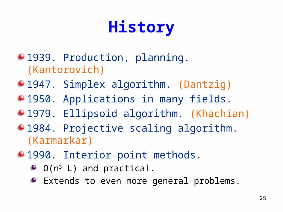
1939. Production, planning. (Kantorovich)1947. Simplex algorithm. (Dantzig)1950. Applications in many fields.
Military logistics. Operations research. Control theory. Filter design. Structural optimization.
23
History
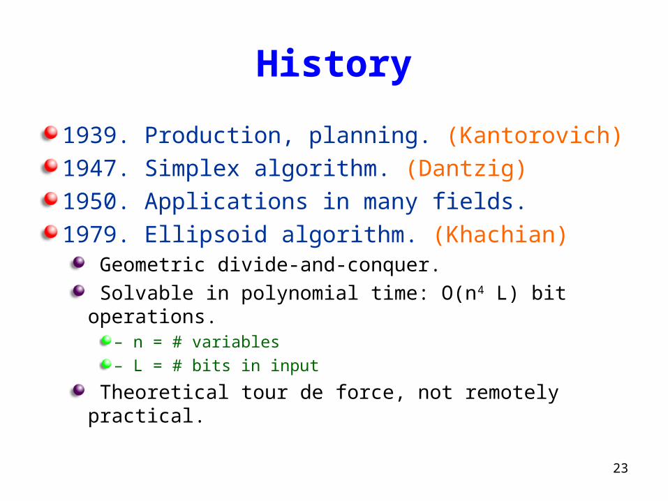
1939. Production, planning. (Kantorovich)1947. Simplex algorithm. (Dantzig)1950. Applications in many fields.1979. Ellipsoid algorithm. (Khachian)
Geometric divide-and-conquer. Solvable in polynomial time: O(n4 L) bit operations.
– n = # variables– L = # bits in input
Theoretical tour de force, not remotely practical.
24
History
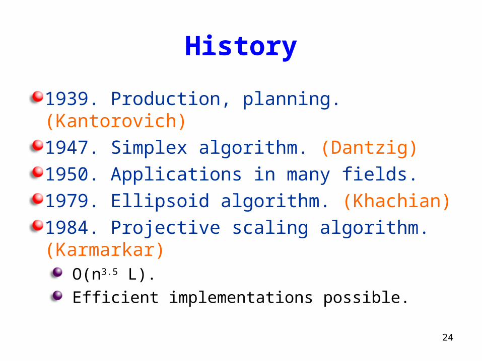
1939. Production, planning. (Kantorovich)1947. Simplex algorithm. (Dantzig)1950. Applications in many fields.1979. Ellipsoid algorithm. (Khachian)1984. Projective scaling algorithm. (Karmarkar)
O(n3.5 L). Efficient implementations possible.
25
History
1939. Production, planning. (Kantorovich)1947. Simplex algorithm. (Dantzig)1950. Applications in many fields.1979. Ellipsoid algorithm. (Khachian)1984. Projective scaling algorithm. (Karmarkar)1990. Interior point methods.
O(n3 L) and practical. Extends to even more general problems.

26
Perspective
LP is near the deep waters of NP-completeness.
Solvable in polynomial time. Known for less than 28 years.
Integer linear programming. LP with integrality requirement. NP-hard.
27
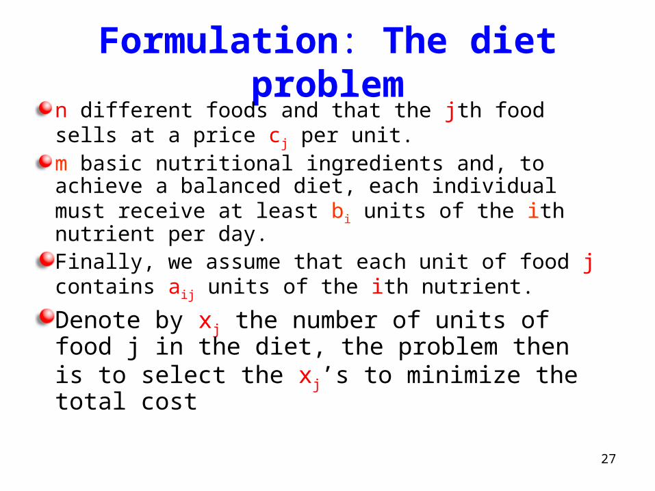
Formulation: The diet problemn different foods and that the jth food sells at a price cj per unit. m basic nutritional ingredients and, to achieve a balanced diet, each individual must receive at least bi units of the ith nutrient per day.
Finally, we assume that each unit of food j contains aij units of the ith nutrient.
Denote by xj the number of units of food j in the diet, the problem then is to select the xj’s to minimize the total cost
28
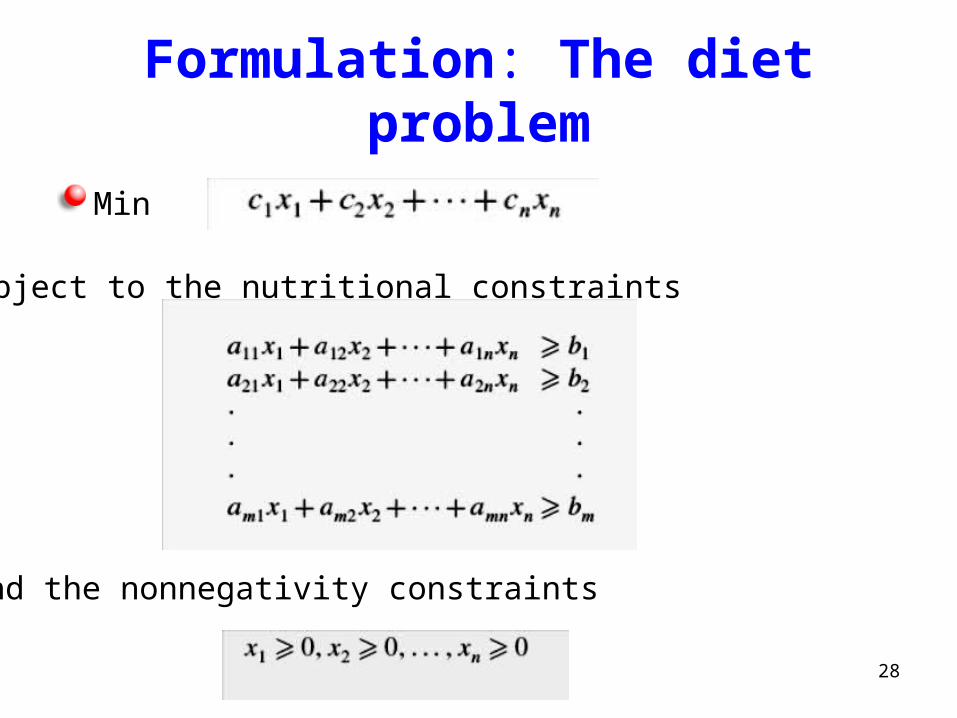
Formulation: The diet problem
Min
Subject to the nutritional constraints
and the nonnegativity constraints
29
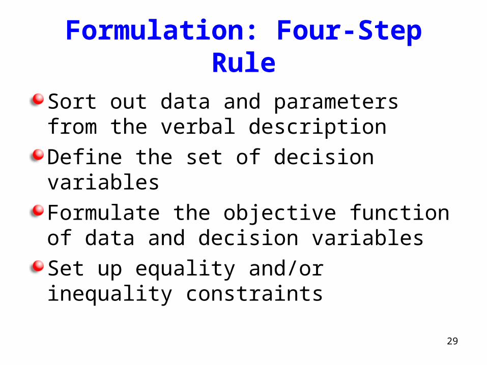
Formulation: Four-Step Rule
Sort out data and parameters from the verbal description
Define the set of decision variables
Formulate the objective function of data and decision variables
Set up equality and/or inequality constraints
30
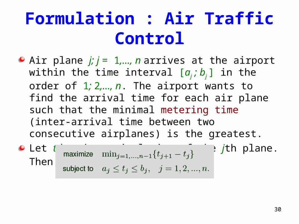
Formulation : Air Traffic Control
Air plane j; j = 1,..., n arrives at the airport within the time interval [aj ; bj ] in the order of 1; 2,..., n. The airport wants to find the arrival time for each air plane such that the minimal metering time (inter-arrival time between two consecutive airplanes) is the greatest.Let tj be the arrival time of the jth plane. Then, the problem is
31
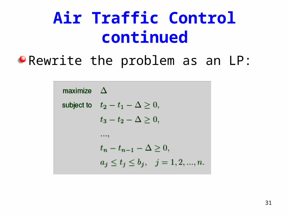
Air Traffic Control continued
Rewrite the problem as an LP:
32
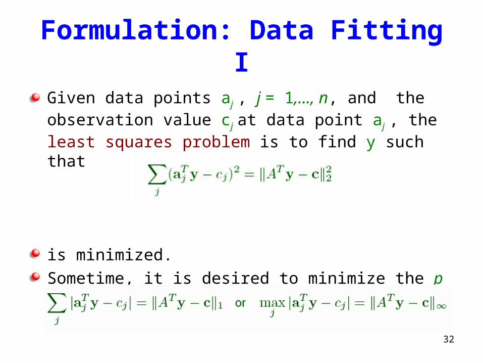
Formulation: Data Fitting I
Given data points aj , j = 1,..., n, and the observation value cj at data point aj , the least squares problem is to find y such that
is minimized.Sometime, it is desired to minimize the p norm, where p = 1 or p = ∞
33
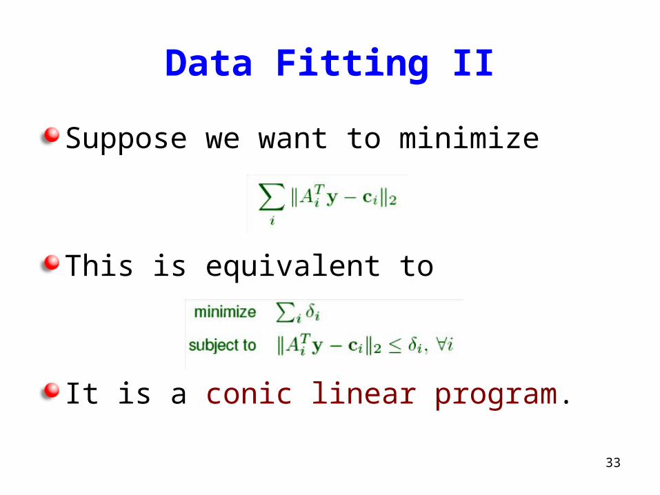
Data Fitting II
Suppose we want to minimize
This is equivalent to
It is a conic linear program.

34
Sensor Network Localization
There are n distinct sensor points in Rd whose locations are to be determined,
Given m fixed points (called the anchor points) whose locations are known as a1, a2,...,am.
dij the Euclidean distance between the ith and jth sensor points, and the distance between the ith sensor and kth anchor point
2 2
, ,
|| || || ||
. .
|| ||
|| ||
i j i ki j k
i j ij
i k ik
Min x x x a
s t
x x d rd
x a d rd
ikd
35
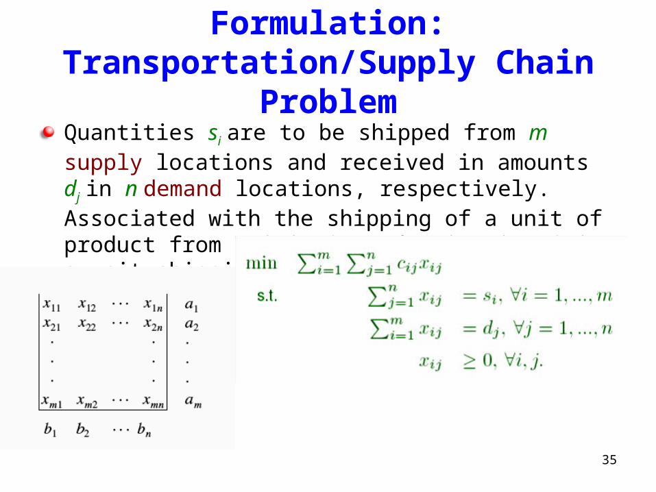
Formulation: Transportation/Supply Chain Problem
Quantities si are to be shipped from m supply locations and received in amounts dj in n demand locations, respectively. Associated with the shipping of a unit of product from origin i to destination j is a unit shipping cost cij .
36
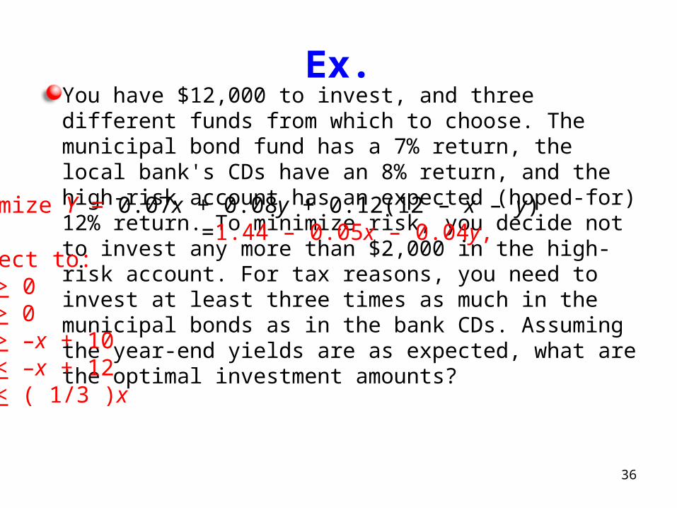
Ex.You have $12,000 to invest, and three different funds from which to choose. The municipal bond fund has a 7% return, the local bank's CDs have an 8% return, and the high-risk account has an expected (hoped-for) 12% return. To minimize risk, you decide not to invest any more than $2,000 in the high-risk account. For tax reasons, you need to invest at least three times as much in the municipal bonds as in the bank CDs. Assuming the year-end yields are as expected, what are the optimal investment amounts?
Maximize Y = 0.07x + 0.08y + 0.12(12 – x – y) =1.44 – 0.05x – 0.04y, subject to: x > 0 y > 0 y > –x + 10 y < –x + 12 y < ( 1/3 )x
37
Maximizing Ad-auctions revenue
There is a set I of n buyers, each buyer i has a known daily budget of B(i).Upon arrival of a product j, each buyer provides a bid b(i, j) for buying item jThe revenue received from each buyer is defined to be the minimum between the sum of the costs of the products allocated to a buyer (times the fraction allocated) and the total budget of the buyer. The objective is to maximize the total revenue of the seller.

38
Maximizing Ad-auctions revenue
Let y(i, j) denote the fraction of product j allocated to buyer i
39
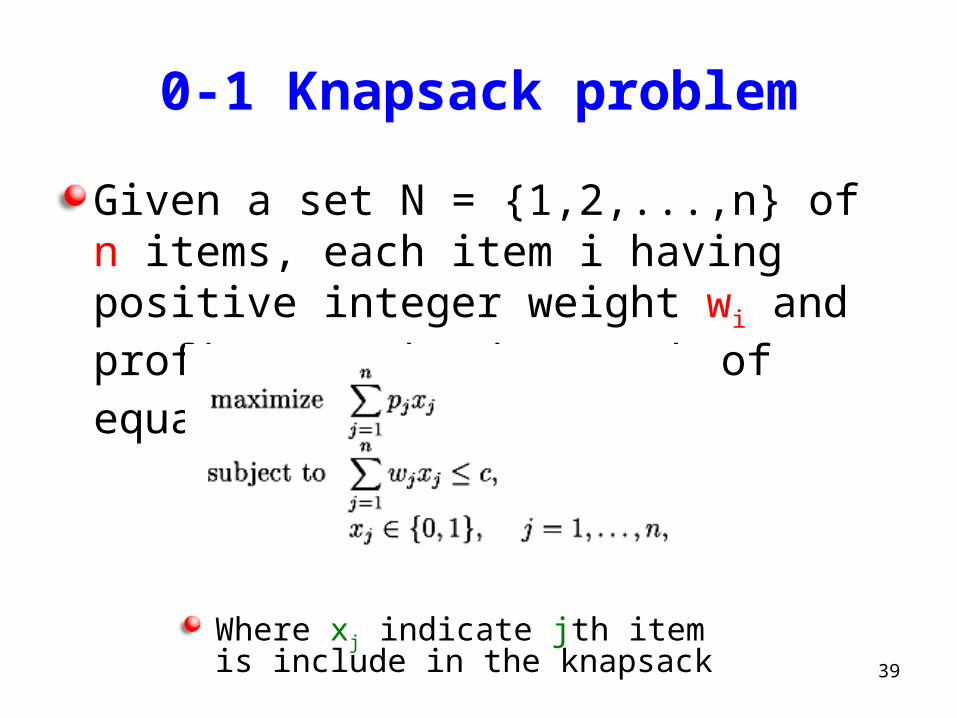
0-1 Knapsack problem
Given a set N = {1,2,...,n} of n items, each item i having positive integer weight wi and profit pi and a knapsack of equal capacity c.
Where xj indicate jth item is include in the knapsack
40
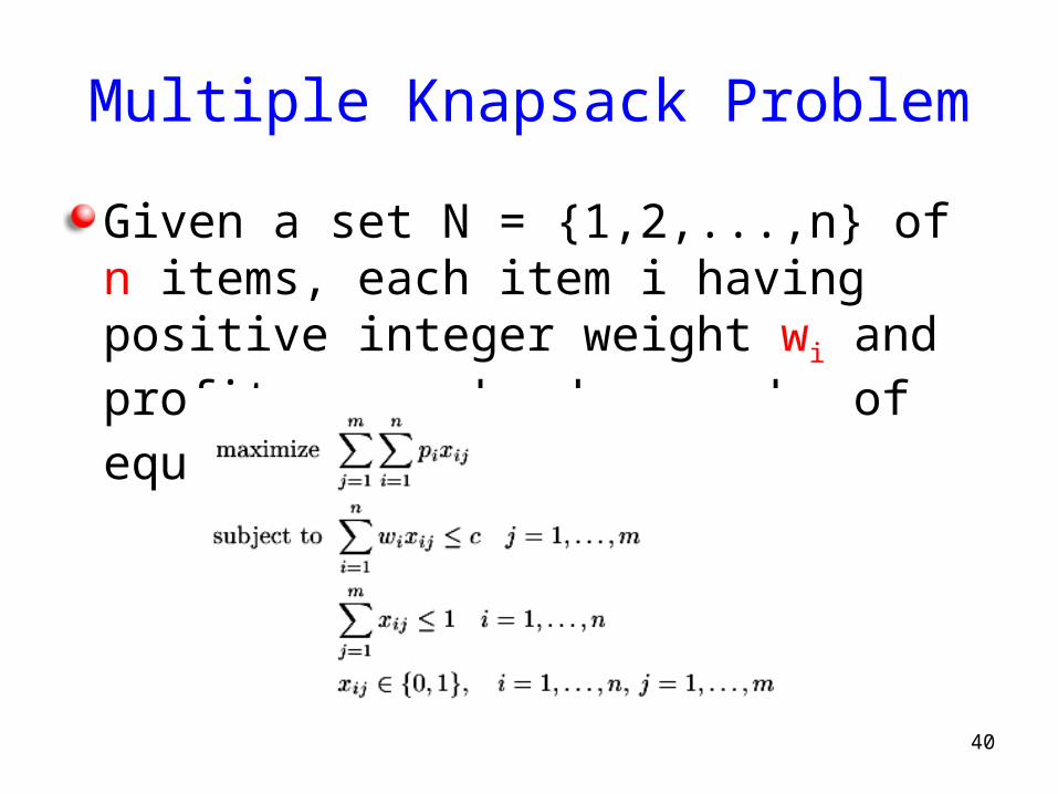
Multiple Knapsack Problem
Given a set N = {1,2,...,n} of n items, each item i having positive integer weight wi and profit pi and m knapsacks of equal capacity c
41
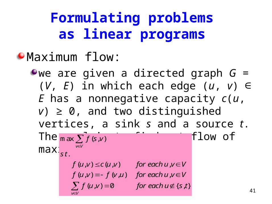
Formulating problems as linear programs
Maximum flow:we are given a directed graph G = (V, E) in which each edge (u, v) ∈ E has a nonnegative capacity c(u, v) ≥ 0, and two distinguished vertices, a sink s and a source t. The goal is to find s-t flow of maximum value.
max ( , )
. .
( , ) ( , ) ,
( , ) ( , ) ,
( , ) 0 { , }
v V
v V
f s v
s t
f u v c u v for each u v V
f u v f v u for each u v V
f u v for each u s t

42
Dynamic TCP-Acknowledgement
A stream of packets arrives at a destination from a source. The source needs to get an acknowledgement for each of the packets, however, it is possible to acknowledge several packets by a single acknowledgement message. The objective function is to minimize the number of acknowledgement messages sent along with the sum of latencies of the packets
43
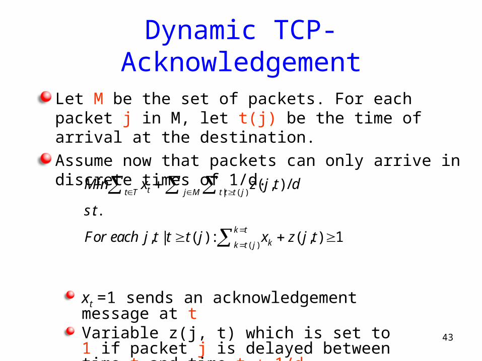
Dynamic TCP-Acknowledgement
Let M be the set of packets. For each packet j in M, let t(j) be the time of arrival at the destination.
Assume now that packets can only arrive in discrete times of 1/d.
| ( )
( )
( , ) /
. .
, | ( ) : ( , ) 1
tt T j M t t t j
k t
kk t j
Min x z j t d
s t
For each j t t t j x z j t
xt =1 sends an acknowledgement message at tVariable z(j, t) which is set to 1 if packet j is delayed between time t and time t + 1/d
44
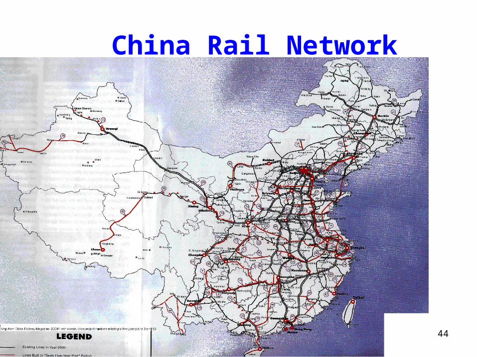
China Rail Network

45
Maximum Flow and Minimum Cut
Max flow and min cut.
Two very rich algorithmic problems.
Cornerstone problems in combinatorial optimization.
Beautiful mathematical duality.
46
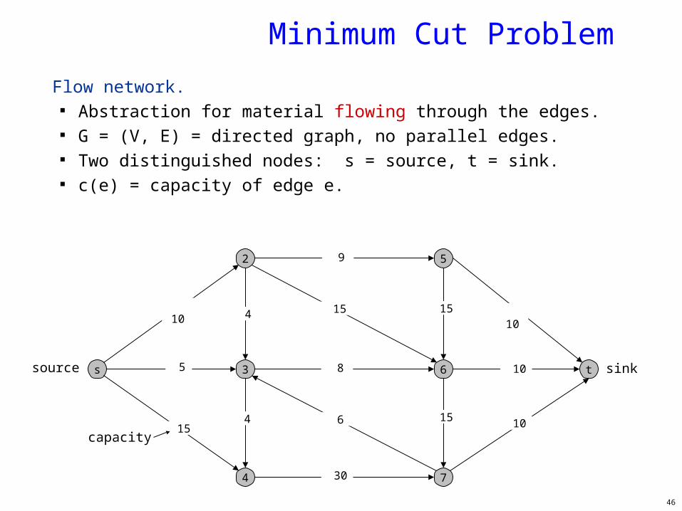
Flow network. Abstraction for material flowing through the edges. G = (V, E) = directed graph, no parallel edges. Two distinguished nodes: s = source, t = sink. c(e) = capacity of edge e.
Minimum Cut Problem
s
2
3
4
5
6
7
t
15
5
30
15
10
8
15
9
6 10
10
10 15 4
4
capacity
source sink
47
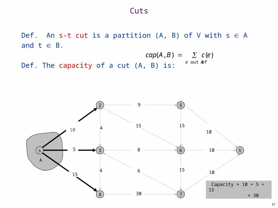
Def. An s-t cut is a partition (A, B) of V with s A and t B.
Def. The capacity of a cut (A, B) is:
Cuts
s
2
3
4
5
6
7
t
15
5
30
15
10
8
15
9
6 10
10
10 15 4
4
Capacity = 10 + 5 + 15 = 30
A
cap( A, B) c(e)e out of A
48
s
2
3
4
5
6
7
t
15
5
30
15
10
8
15
9
6 10
10
10 15 4
4 A
Cuts
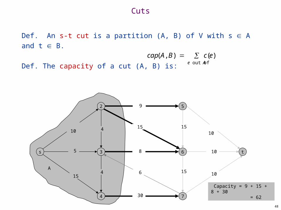
Def. An s-t cut is a partition (A, B) of V with s A and t B.
Def. The capacity of a cut (A, B) is:
cap( A, B) c(e)e out of A
Capacity = 9 + 15 + 8 + 30 = 62
49
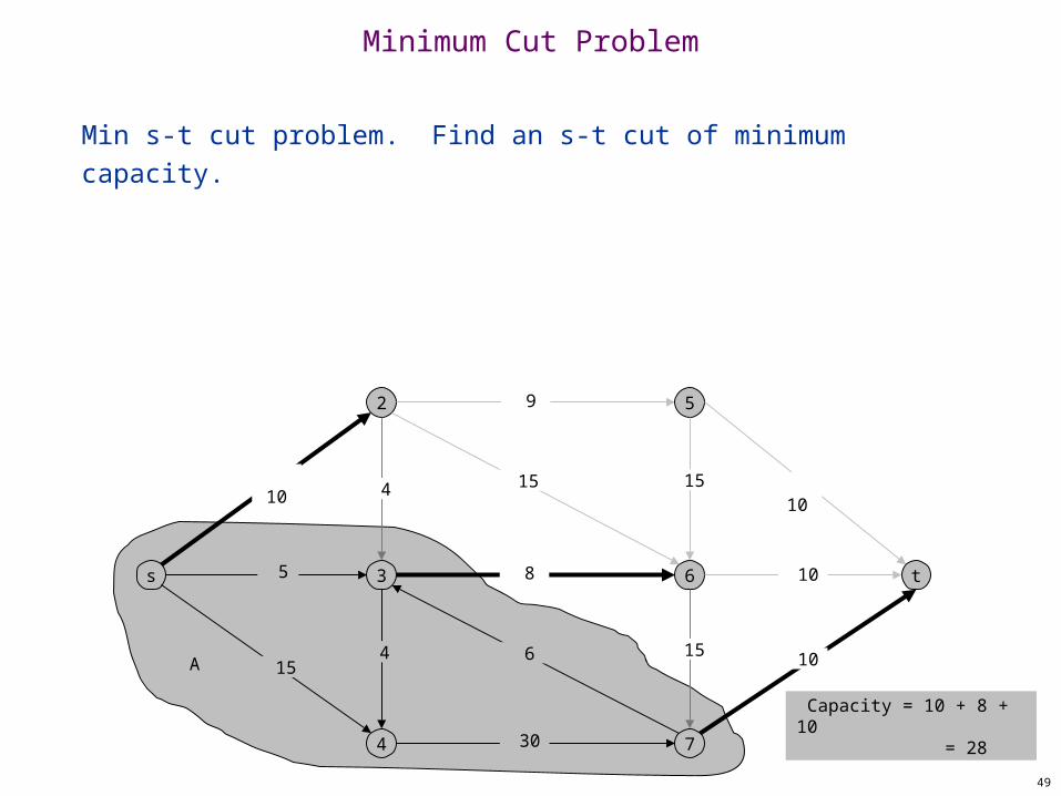
Min s-t cut problem. Find an s-t cut of minimum capacity.
Minimum Cut Problem
s
2
3
4
5
6
7
t
15
5
30
15
10
8
15
9
6 10
10
10 15 4
4 A
Capacity = 10 + 8 + 10 = 28
50
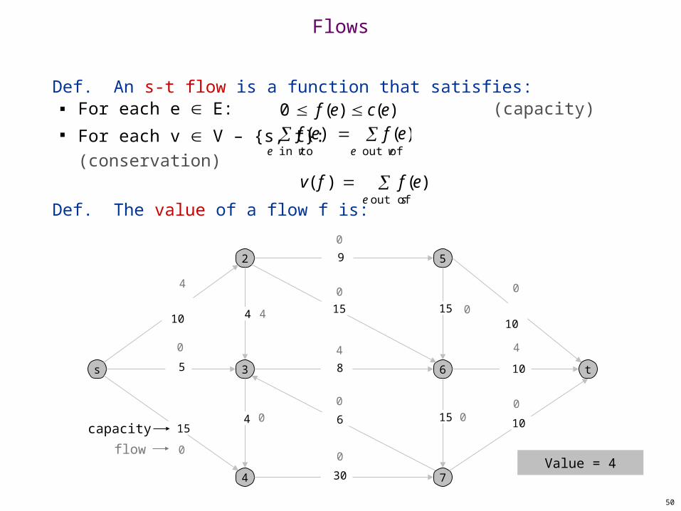
Def. An s-t flow is a function that satisfies: For each e E: (capacity) For each v V – {s, t}: (conservation)
Def. The value of a flow f is:
Flows
4
0
0
0
0 0
0 4 4
0
0
0
Value = 40
f (e)e in to v f (e)
e out of v
0 f (e) c(e)
capacity
flow
s
2
3
4
5
6
7
t
15
5
30
15
10
8
15
9
6 10
10
10 15 4
4 0
v( f ) f (e) e out of s
.
4
51
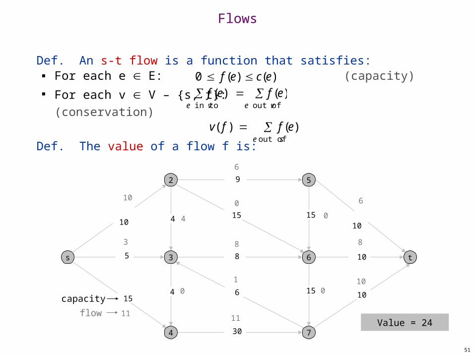
Def. An s-t flow is a function that satisfies: For each e E: (capacity) For each v V – {s, t}: (conservation)
Def. The value of a flow f is:
Flows
10
6
6
11
1 10
3 8 8
0
0
0
11
capacity
flow
s
2
3
4
5
6
7
t
15
5
30
15
10
8
15
9
6 10
10
10 15 4
4 0
Value = 24
f (e)e in to v f (e)
e out of v
0 f (e) c(e)
v( f ) f (e) e out of s
.
4
52
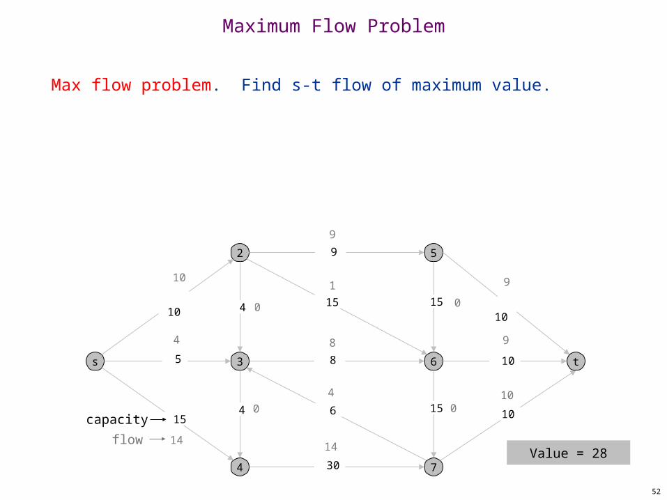
Max flow problem. Find s-t flow of maximum value.
Maximum Flow Problem
10
9
9
14
4 10
4 8 9
1
0 0
0
14
capacity
flow
s
2
3
4
5
6
7
t
15
5
30
15
10
8
15
9
6 10
10
10 15 4
4 0
Value = 28
53
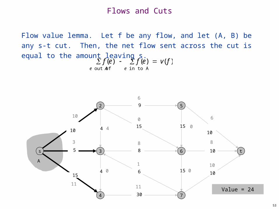
Flow value lemma. Let f be any flow, and let (A, B) be any s-t cut. Then, the net flow sent across the cut is equal to the amount leaving s.
Flows and Cuts
10
6
6
11
1 10
3 8 8
0
0
0
11
s
2
3
4
5
6
7
t
15
5
30
15
10
8
15
9
6 10
10
10 15 4
4 0
Value = 24
f (e)e out of A
f (e)e in to A
v( f )
4
A

54
Flow value lemma. Let f be any flow, and let (A, B) be any s-t cut. Then, the net flow sent across the cut is equal to the amount leaving s.
Flows and Cuts
10
6
6
1 10
3 8 8
0
0
0
11
s
2
3
4
5
6
7
t
15
5
30
15
10
8
15
9
6 10
10
10 15 4
4 0
f (e)e out of A
f (e)e in to A
v( f )
Value = 6 + 0 + 8 - 1 + 11 = 24
4
11
A
55
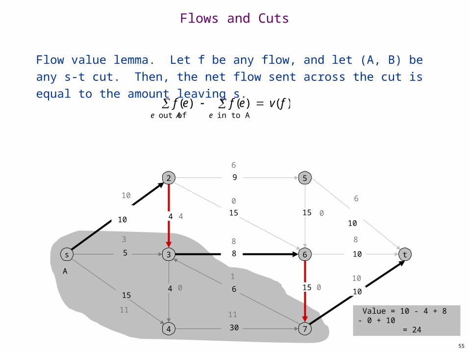
Flow value lemma. Let f be any flow, and let (A, B) be any s-t cut. Then, the net flow sent across the cut is equal to the amount leaving s.
Flows and Cuts
10
6
6
11
1 10
3 8 8
0
0
0
11
s
2
3
4
5
6
7
t
15
5
30
15
10
8
15
9
6 10
10
10 15 4
4 0
f (e)e out of A
f (e)e in to A
v( f )
Value = 10 - 4 + 8 - 0 + 10 = 24
4
A
56
Flows and Cuts
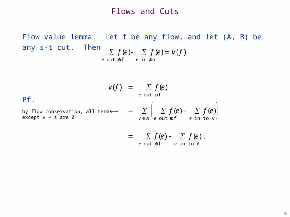
Flow value lemma. Let f be any flow, and let (A, B) be any s-t cut. Then
Pf.
f (e)e out of A
f (e) v( f )e in to A
.
v( f ) f (e)e out of s
v A f (e)
e out of v f (e)
e in to v
f (e)e out of A
f (e).e in to A
by flow conservation, all termsexcept v = s are 0
57
Flows and Cuts
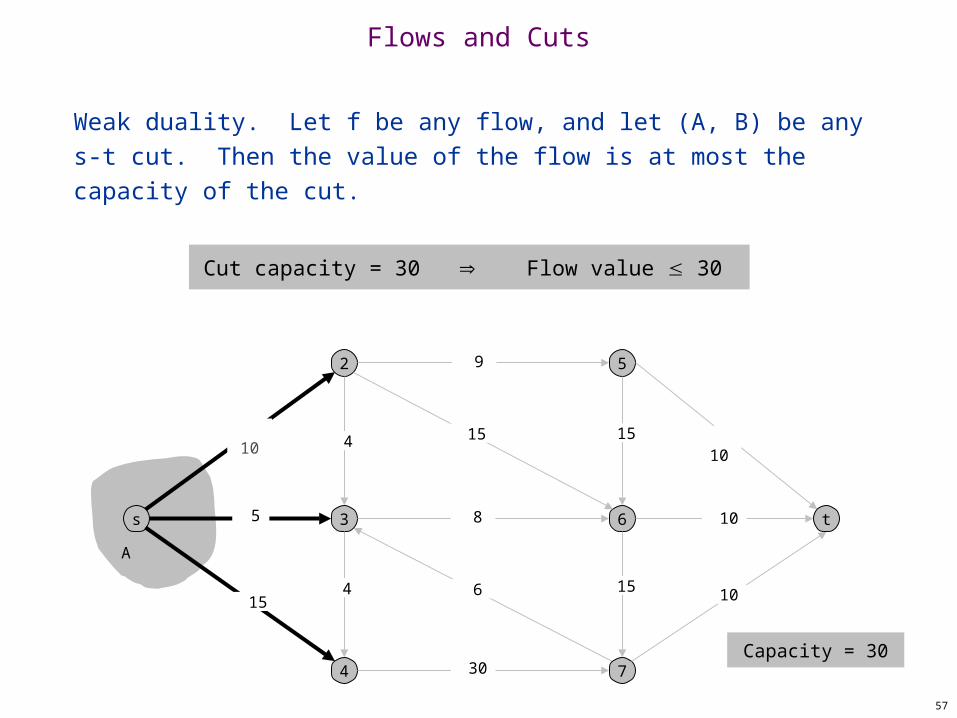
Weak duality. Let f be any flow, and let (A, B) be any s-t cut. Then the value of the flow is at most the capacity of the cut.
Cut capacity = 30 Flow value 30
s
2
3
4
5
6
7
t
15
5
30
15
10
8
15
9
6 10
10
10 15 4
4
Capacity = 30
A
58
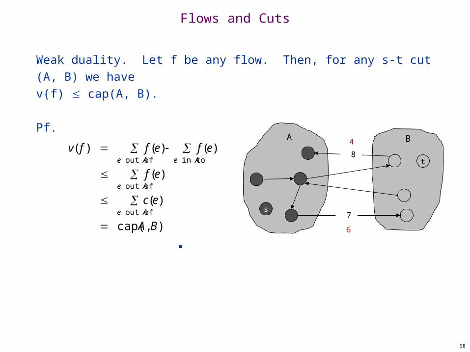
Weak duality. Let f be any flow. Then, for any s-t cut (A, B) we havev(f) cap(A, B).
Pf.
▪
Flows and Cuts
v( f ) f (e)e out of A
f (e)e in to A
f (e)e out of A
c(e)e out of A
cap(A, B)
s
t
A B
7
6
8
4
59
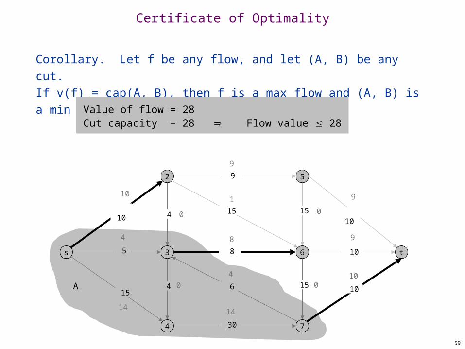
Certificate of Optimality
Corollary. Let f be any flow, and let (A, B) be any cut.If v(f) = cap(A, B), then f is a max flow and (A, B) is a min cut.
Value of flow = 28Cut capacity = 28 Flow value 28
10
9
9
14
4 10
4 8 9
1
0 0
0
14
s
2
3
4
5
6
7
t
15
5
30
15
10
8
15
9
6 10
10
10 15 4
4 0A

Bipartite Matching
61
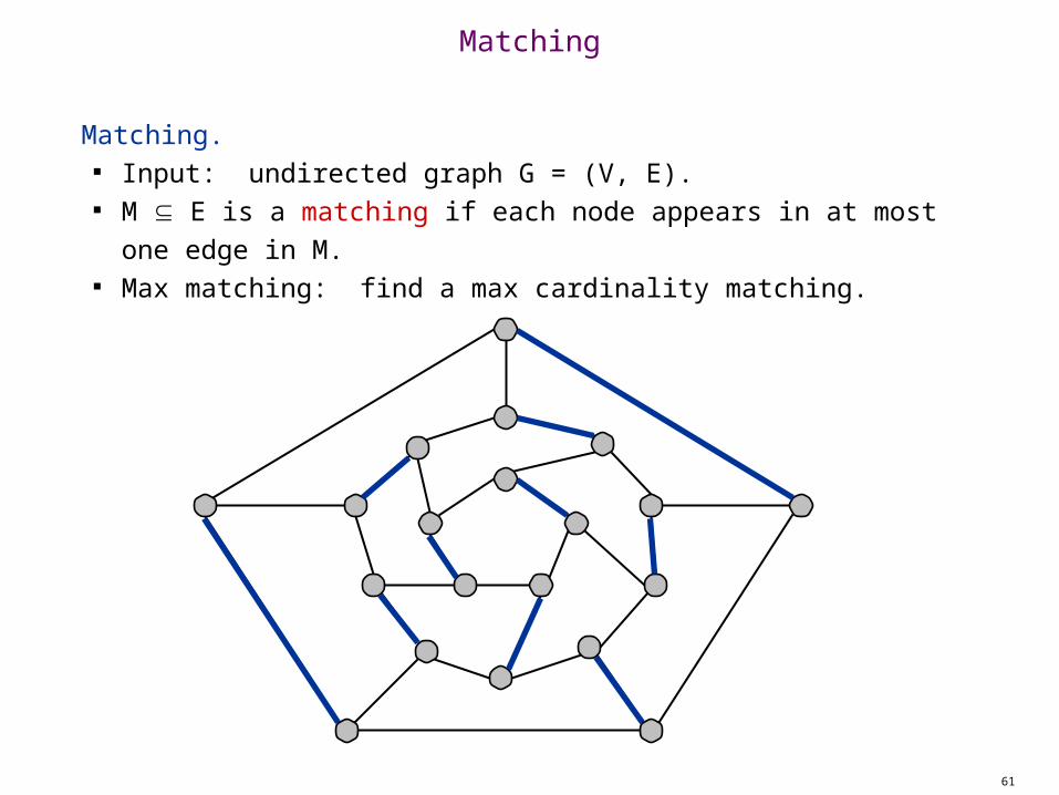
Matching. Input: undirected graph G = (V, E). M E is a matching if each node appears in at most one edge
in M. Max matching: find a max cardinality matching.
Matching

62
Bipartite Matching
Bipartite matching. Input: undirected, bipartite graph G = (L R, E). M E is a matching if each node appears in at most one edge
in M. Max matching: find a max cardinality matching.
1
3
5
1'
3'
5'
2
4
2'
4'
matching
1-2', 3-1', 4-5'
RL
63
Bipartite Matching
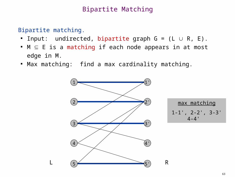
Bipartite matching. Input: undirected, bipartite graph G = (L R, E). M E is a matching if each node appears in at most edge in M. Max matching: find a max cardinality matching.
1
3
5
1'
3'
5'
2
4
2'
4'
RL
max matching
1-1', 2-2', 3-3' 4-4'
64
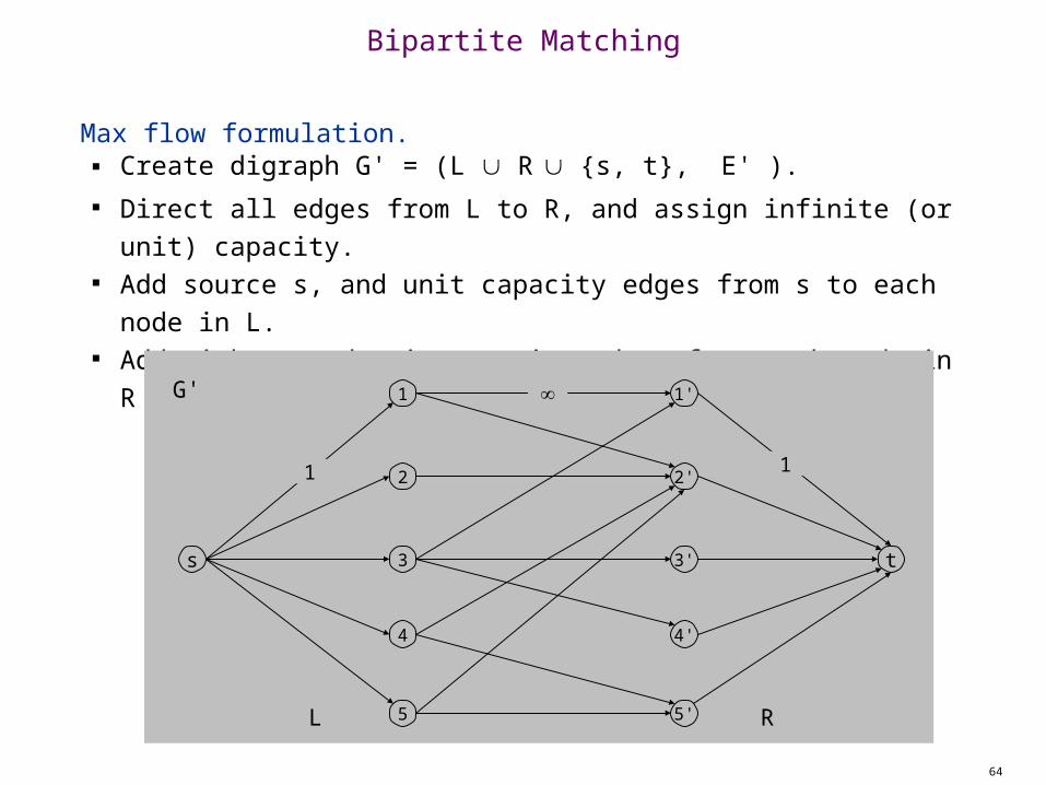
Max flow formulation. Create digraph G' = (L R {s, t}, E' ). Direct all edges from L to R, and assign infinite (or unit)
capacity. Add source s, and unit capacity edges from s to each node in L. Add sink t, and unit capacity edges from each node in R to t.
Bipartite Matching
s
1
3
5
1'
3'
5'
t
2
4
2'
4'
1 1
RL
G'
65
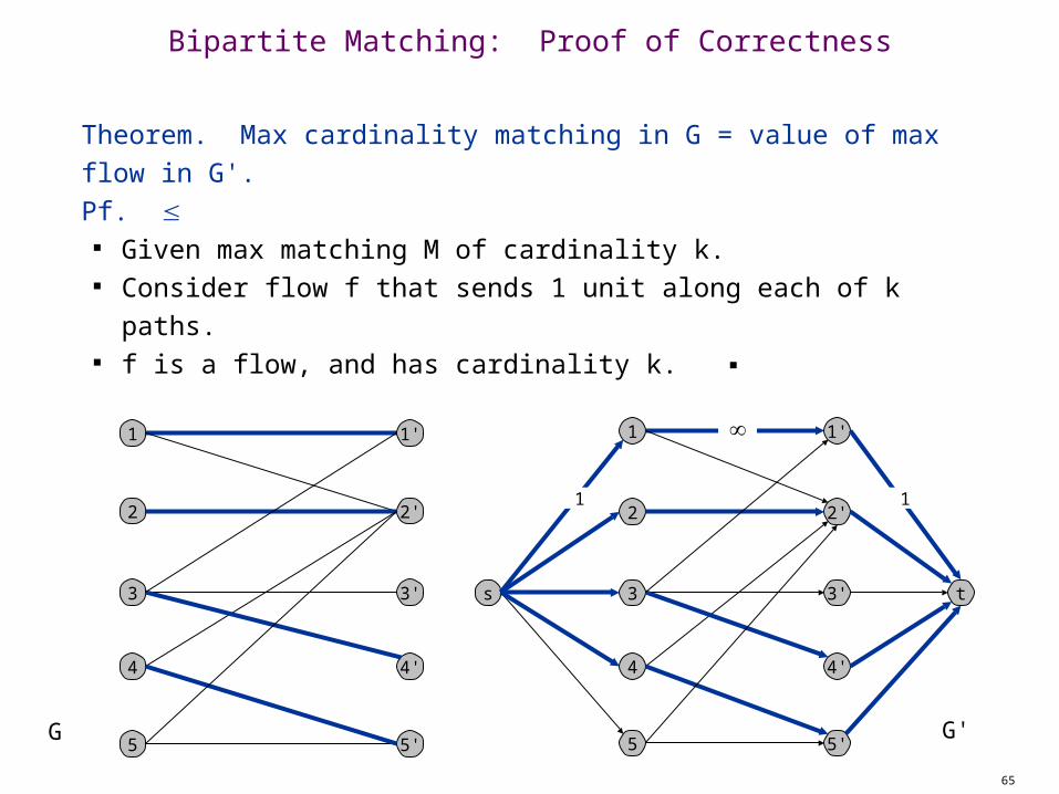
Theorem. Max cardinality matching in G = value of max flow in G'.Pf.
Given max matching M of cardinality k. Consider flow f that sends 1 unit along each of k paths. f is a flow, and has cardinality k. ▪
Bipartite Matching: Proof of Correctness
s
1
3
5
1'
3'
5'
t
2
4
2'
4'
1 1
1
3
5
1'
3'
5'
2
4
2'
4'
G'G
66
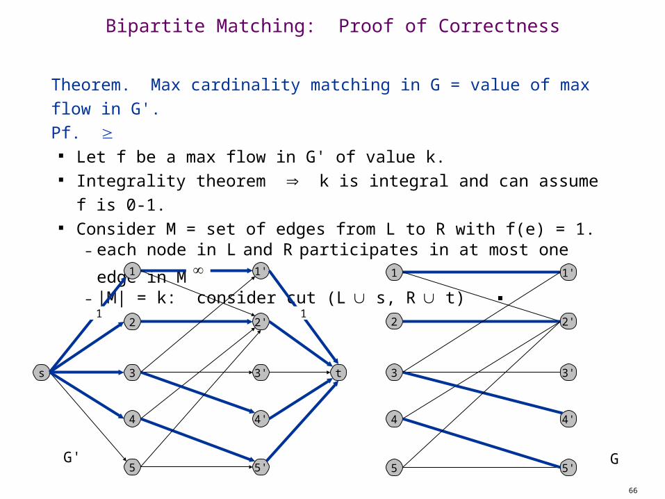
Theorem. Max cardinality matching in G = value of max flow in G'.Pf.
Let f be a max flow in G' of value k. Integrality theorem k is integral and can assume f is 0-1. Consider M = set of edges from L to R with f(e) = 1.
– each node in L and R participates in at most one edge in M– |M| = k: consider cut (L s, R t) ▪
Bipartite Matching: Proof of Correctness
1
3
5
1'
3'
5'
2
4
2'
4'
G
s
1
3
5
1'
3'
5'
t
2
4
2'
4'
1 1
G'

Disjoint Paths

68
Disjoint path problem. Given a digraph G = (V, E) and two nodes s and t, find the max number of edge-disjoint s-t paths.
Def. Two paths are edge-disjoint if they have no edge in common.
Ex: communication networks.
s
2
3
4
Edge Disjoint Paths
5
6
7
t
69
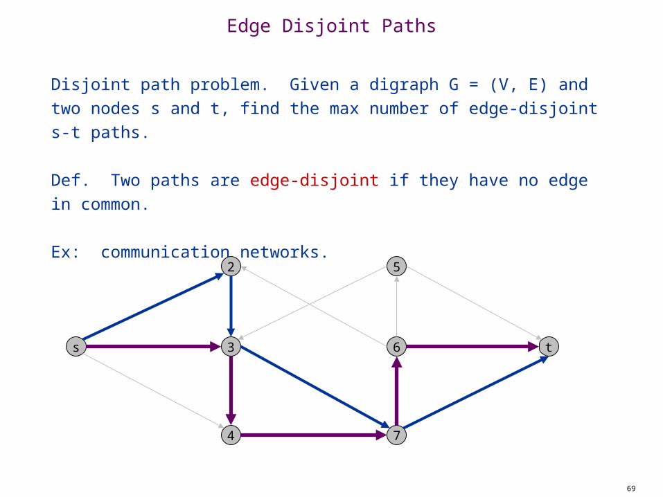
Disjoint path problem. Given a digraph G = (V, E) and two nodes s and t, find the max number of edge-disjoint s-t paths.
Def. Two paths are edge-disjoint if they have no edge in common.
Ex: communication networks.
s
2
3
4
Edge Disjoint Paths
5
6
7
t
70
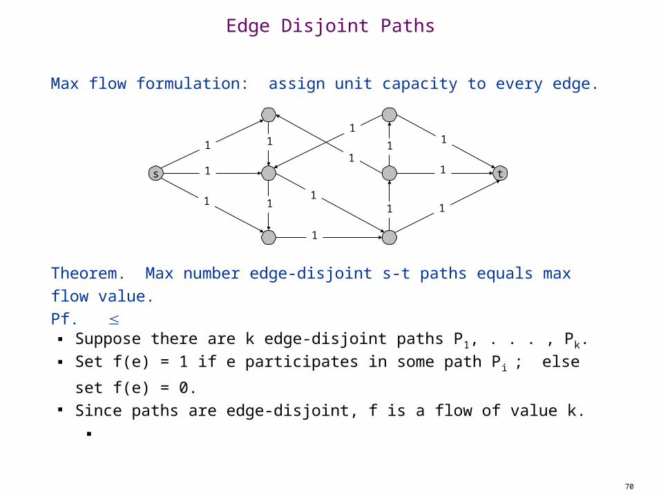
Max flow formulation: assign unit capacity to every edge.
Theorem. Max number edge-disjoint s-t paths equals max flow value.Pf.
Suppose there are k edge-disjoint paths P1, . . . , Pk. Set f(e) = 1 if e participates in some path Pi ; else set f(e) = 0. Since paths are edge-disjoint, f is a flow of value k. ▪
Edge Disjoint Paths
s t
1
1
1
1
1
1
11
1
1
1
1
1
1

71
Max flow formulation: assign unit capacity to every edge.
Theorem. Max number edge-disjoint s-t paths equals max flow value.Pf.
Suppose max flow value is k. Integrality theorem there exists 0-1 flow f of value k. Consider edge (s, u) with f(s, u) = 1.
– by conservation, there exists an edge (u, v) with f(u, v) = 1– continue until reach t, always choosing a new edge
Produces k (not necessarily simple) edge-disjoint paths. ▪
Edge Disjoint Paths
s t
1
1
1
1
1
1
11
1
1
1
1
1
1
can eliminate cycles to get simple paths if desired

72
Network connectivity. Given a digraph G = (V, E) and two nodes s and t, find min number of edges whose removal disconnects t from s.
Def. A set of edges F E disconnects t from s if all s-t paths uses at least on edge in F.
Network Connectivity
s
2
3
4
5
6
7
t
73
Edge Disjoint Paths and Network Connectivity
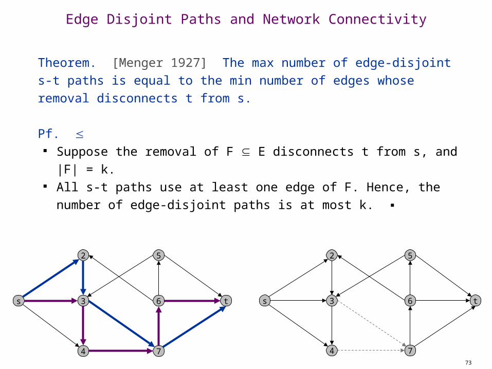
Theorem. [Menger 1927] The max number of edge-disjoint s-t paths is equal to the min number of edges whose removal disconnects t from s.
Pf. Suppose the removal of F E disconnects t from s, and |F| = k. All s-t paths use at least one edge of F. Hence, the number of
edge-disjoint paths is at most k. ▪
s
2
3
4
5
6
7
t s
2
3
4
5
6
7
t
74
Disjoint Paths and Network Connectivity
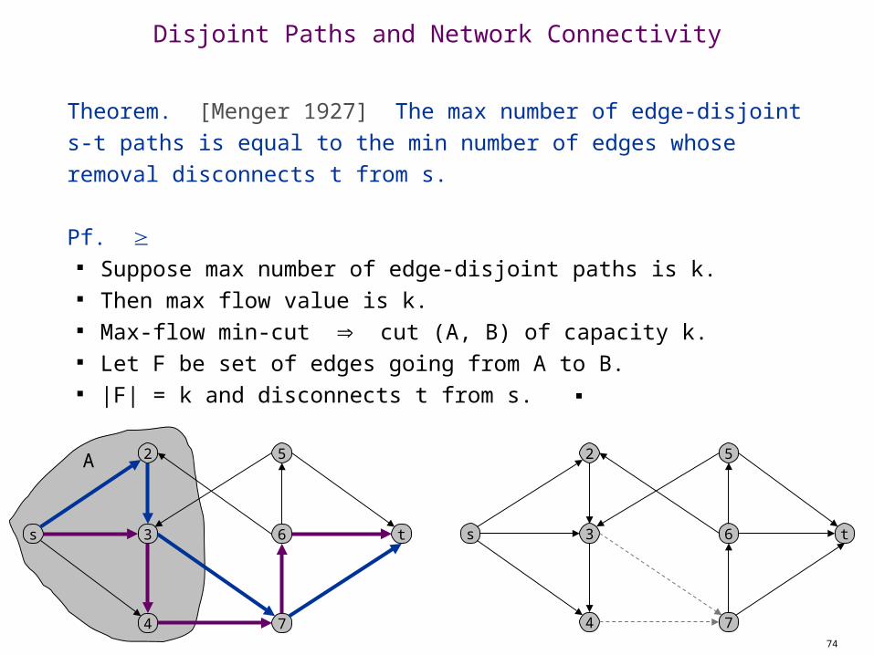
Theorem. [Menger 1927] The max number of edge-disjoint s-t paths is equal to the min number of edges whose removal disconnects t from s.
Pf. Suppose max number of edge-disjoint paths is k. Then max flow value is k. Max-flow min-cut cut (A, B) of capacity k. Let F be set of edges going from A to B. |F| = k and disconnects t from s. ▪
s
2
3
4
5
6
7
t s
2
3
4
5
6
7
t
A
Extensions to Max Flow
76
Circulation with Demands
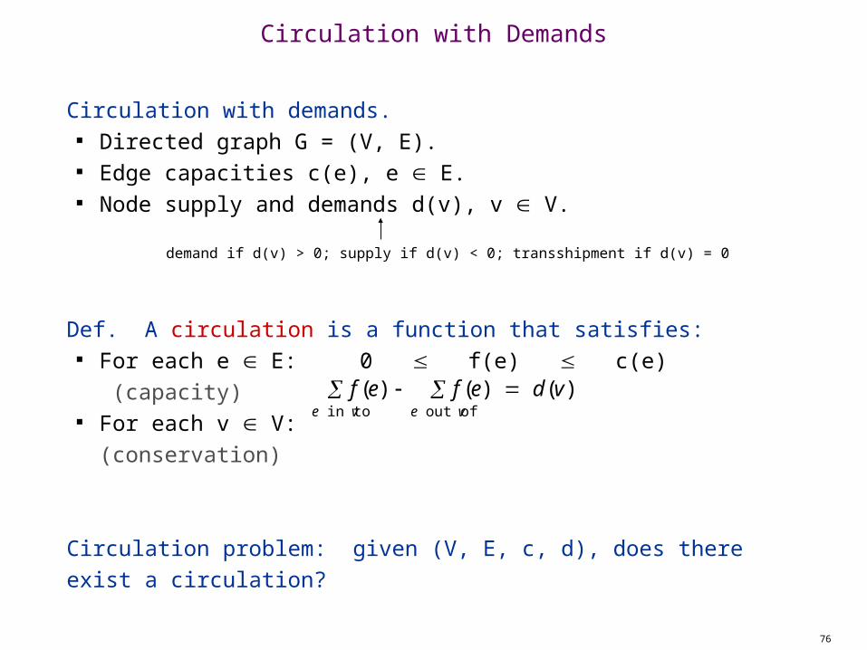
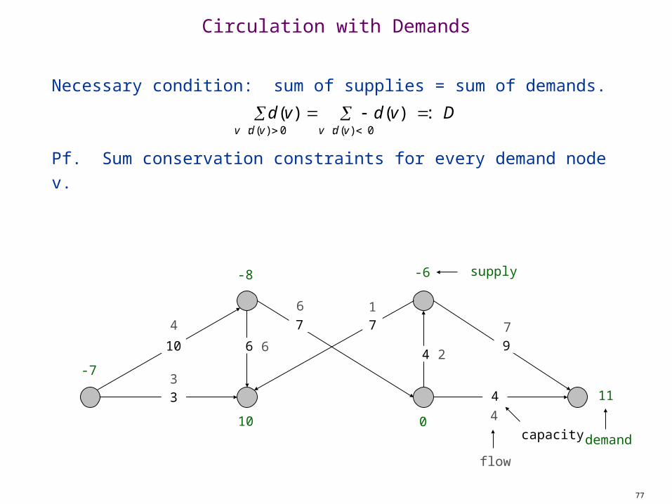
Circulation with demands. Directed graph G = (V, E). Edge capacities c(e), e E. Node supply and demands d(v), v V.
Def. A circulation is a function that satisfies: For each e E: 0 f(e) c(e) (capacity) For each v V: (conservation)
Circulation problem: given (V, E, c, d), does there exist a circulation?
f (e)e in to v
f (e)e out of v
d (v)
demand if d(v) > 0; supply if d(v) < 0; transshipment if d(v) = 0
77
Necessary condition: sum of supplies = sum of demands.
Pf. Sum conservation constraints for every demand node v.
3
10 6
-7
-8
11
-6
4
97
3
10 0
7
4
4
6
6
71
4 2
flow
Circulation with Demands
capacity
d (v)v : d (v) 0
d (v)v : d (v) 0
: D
demand
supply

78
Circulation with Demands
Max flow formulation.
G:
supply
3
10 6
-7
-8
11
-6
4
9
10 0
7
4
7
4
demand

79
Circulation with Demands
Max flow formulation. Add new source s and sink t. For each v with d(v) < 0, add edge (s, v) with capacity -d(v). For each v with d(v) > 0, add edge (v, t) with capacity d(v). Claim: G has circulation iff G' has max flow of value D.
G':
supply
3
10 6 9
0
7
4
7
4
s
t
10 11
7 8 6
saturates all edges
leaving s and entering t
demand

80
Circulation with Demands
Integrality theorem. If all capacities and demands are integers, and there exists a circulation, then there exists one that is integer-valued.
Pf. Follows from max flow formulation and integrality theorem for max flow.
Characterization. Given (V, E, c, d), there does not exists a circulation iff there exists a node partition (A, B) such that vB dv >
cap(A, B)
Pf idea. Look at min cut in G'.
demand by nodes in B exceeds supply
of nodes in B plus max capacity of
edges going from A to B

Project Selection

82
Project Selection
Projects with prerequisites. Set P of possible projects. Project v has associated revenue pv.
– some projects generate money: create interactive e-commerce
interface, redesign web page
– others cost money: upgrade computers, get site license Set of prerequisites E. If (v, w) E, can't do project v and
unless also do project w. A subset of projects A P is feasible if the prerequisite of every
project in A also belongs to A.
Project selection. Choose a feasible subset of projects to maximize revenue.
can be positive or negative

83
Project Selection: Prerequisite Graph
Prerequisite graph. Include an edge from v to w if can't do v without also doing w. {v, w, x} is feasible subset of projects. {v, x} is infeasible subset of projects.
v
w
xv
w
x
feasible infeasible
84
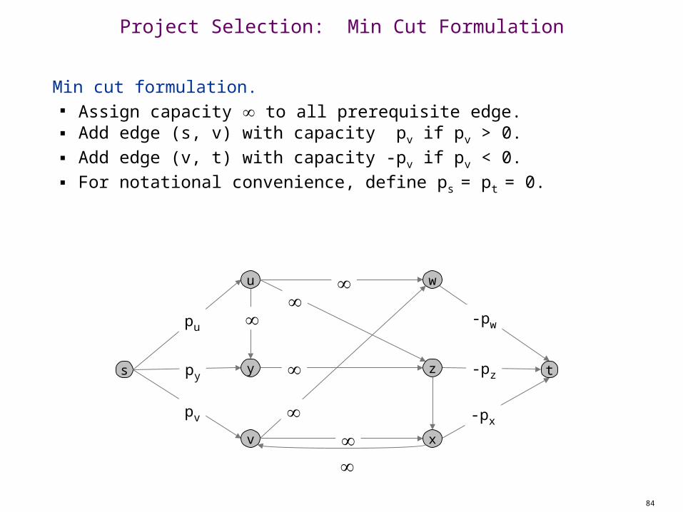
Min cut formulation. Assign capacity to all prerequisite edge. Add edge (s, v) with capacity -pv if pv > 0. Add edge (v, t) with capacity -pv if pv < 0. For notational convenience, define ps = pt = 0.
s t
-pw
u
v
w
x
y z
Project Selection: Min Cut Formulation
pv -px
py
pu
-pz
85
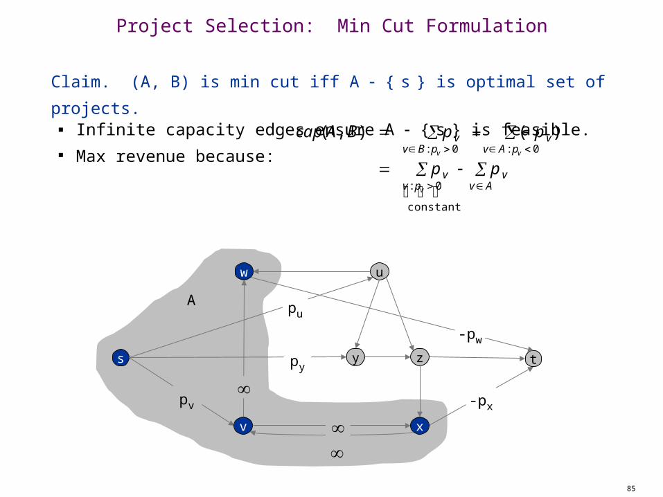
Claim. (A, B) is min cut iff A { s } is optimal set of projects. Infinite capacity edges ensure A { s } is feasible. Max revenue because:
s t
-pw
u
v
w
x
y z
Project Selection: Min Cut Formulation
pv -px
cap(A, B) p vv B: pv 0
( p v)v A: pv 0
p vv : pv 0
constant
p vv A
py
pu
A