1

Lecture 8Lecture 8Second order circuits (i).

Linear time invariant RLC-circuits,

•zero-input response.

•Energy and Q factor

Linear time invariant RLC-circuits, zero-state response

•Step response,

•Impulse response

The State-space approach

•state equations and trajectory,

•matrix representation,

•approximate method for the calculation of trajectory,

•state equations and complete response

2

Linear Time-invariant Linear Time-invariant RLCRLC Circuit, Zero-input response Circuit, Zero-input response

iicc ++vvRR

--

+vc-

iiRR

iiLL+vL-

0)0( VvC 0)0( Iil

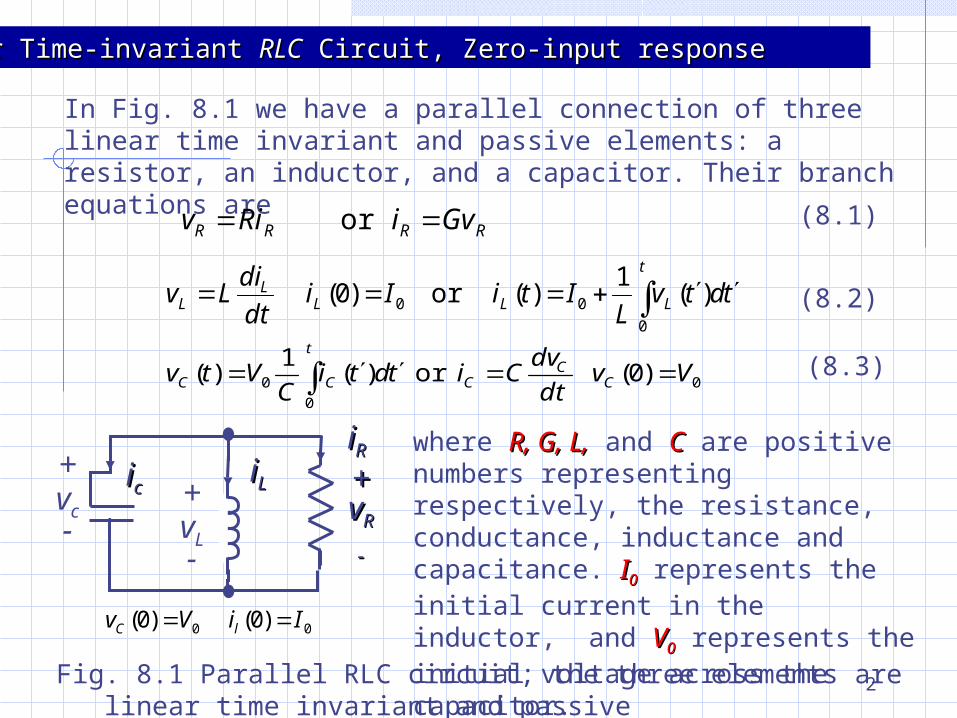
Fig. 8.1 Parallel RLC circuit; the three elements are linear time invariant and passive

In Fig. 8.1 we have a parallel connection of three linear time invariant and passive elements: a resistor, an inductor, and a capacitor. Their branch equations are

RRRR GviRiv or (8.1)

t

LLLL

L tdtvL

ItiIidt

diLv

0

00 )(1

)(or )0( (8.2)

0

0

0 )0( or )(1

)( Vvdt

dvCitdti

CVtv C

tC

CCC (8.3)

where R, G, L,R, G, L, and CC are positive numbers representing respectively, the resistance, conductance, inductance and capacitance. II00 represents the initial current in the inductor, and VV00 represents the initial voltage across the capacitor.

3

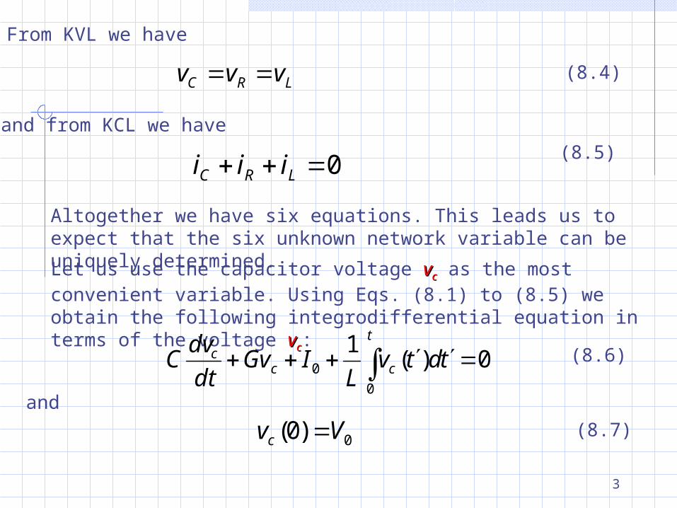
From KVL we have

LRC vvv (8.4)

and from KCL we have

0 LRC iii(8.5)

Altogether we have six equations. This leads us to expect that the six unknown network variable can be uniquely determined. Let us use the capacitor voltage vvcc as the most convenient variable. Using Eqs. (8.1) to (8.5) we obtain the following integrodifferential equation in terms of the voltage vvcc:

t

ccc tdtv

LIGv

dt

dvC

0

0 0)(1 (8.6)

and

0)0( Vvc (8.7)

4

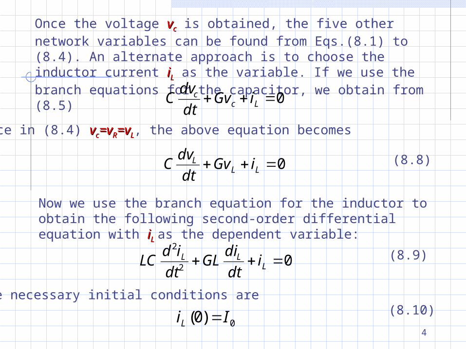
Once the voltage vvcc is obtained, the five other network variables can be found from Eqs.(8.1) to (8.4). An alternate approach is to choose the inductor current iiLL as the variable. If we use the branch equations for the capacitor, we obtain from (8.5)

0 Lcc iGv

dt

dvC

Since in (8.4) vvcc=v=vRR=v=vLL, the above equation becomes

0 LLL iGv

dt

dvC (8.8)

Now we use the branch equation for the inductor to obtain the following second-order differential equation with iiLL as the dependent variable:

02

2

LLL i

dt

diGL

dt

idLC (8.9)

The necessary initial conditions are

0)0( IiL (8.10)

5

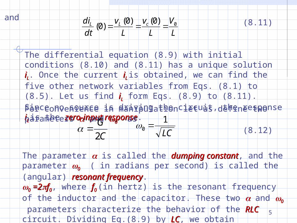
and

L

V

L

v

L

v

dt

di cLL 0)0()0()0( (8.11)

The differential equation (8.9) with initial conditions (8.10) and (8.11) has a unique solution iiLL. Once the current iiL L is obtained, we can find the five other network variables from Eqs. (8.1) to (8.5). Let us find iiLL form Eqs. (8.9) to (8.11). Since no source is driving the circuit, the response iiL L is the zero-input responsezero-input response.For convenience in manipulation let us define two parameters and 00 as

C

G

2 LC

10 (8.12)

The parameter is called the dumping constantdumping constant, and the parameter 00 ( in radians per second) is called the (angular) resonant frequencyresonant frequency. 00 =2 =2ff00, where ff0 0 (in hertz) is the resonant frequency of the inductor and the capacitor. These two and 00 parameters characterize the behavior of the RLCRLC circuit. Dividing Eq.(8.9) by LCLC, we obtain

6

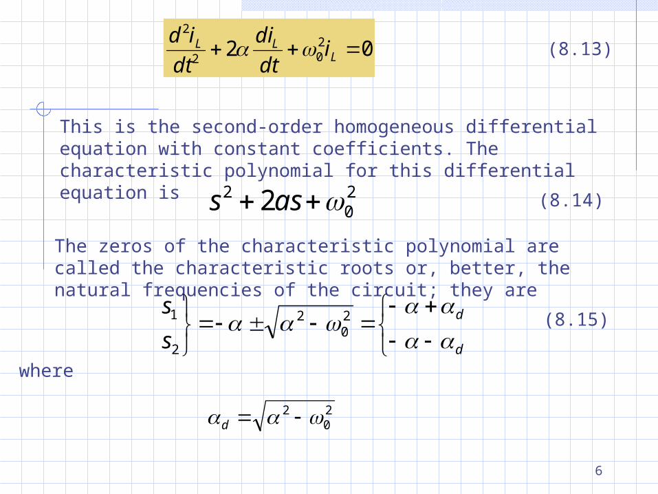
02 202

2

LLL i

dt

di

dt

id (8.13)

This is the second-order homogeneous differential equation with constant coefficients. The characteristic polynomial for this differential equation is

20

2 2 ass (8.14)

The zeros of the characteristic polynomial are called the characteristic roots or, better, the natural frequencies of the circuit; they are

d

d

s

s

20

2

2

1 (8.15)

where

20

2 d

7

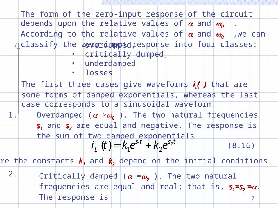
The form of the zero-input response of the circuit depends upon the relative values of and 00 . According to the relative values of and 00 ,we can classify the zero-input response into four classes:• overdumped,

• critically dumped,• underdamped• losses

The first three cases give waveforms iiLL(()) that are some forms of damped exponentials, whereas the last case corresponds to a sinusoidal waveform.

1. Overdamped ( >00 ). The two natural frequencies ss11 and ss22 are equal and negative. The response is the sum of two damped exponentials

tstsL ekekti 21

21)( (8.16)

where the constants kk11 and kk22 depend on the initial conditions.

2. Critically damped ( =00 ). The two natural frequencies are equal and real; that is, ss11=s=s22 = =. The response is

8

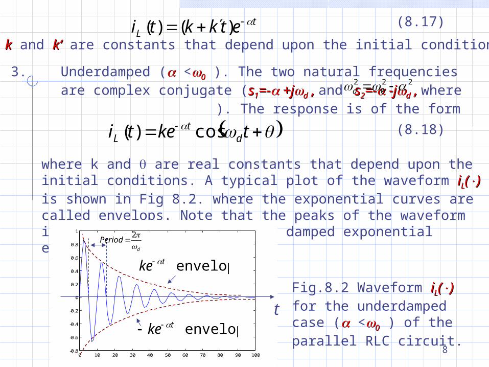
tL etkkti )()( (8.17)

where kk and k‘k‘ are constants that depend upon the initial conditions

3. Underdamped ( <00 ). The two natural frequencies are complex conjugate (ss11=-=- +j +jdd , , and s s22=-=- -j -jdd , , where ). The response is of the form

220

2 d

tketi dt

L cos)( (8.18)

where k and are real constants that depend upon the initial conditions. A typical plot of the waveform iiLL(()) is shown in Fig 8.2. where the exponential curves are called envelops. Note that the peaks of the waveform in amplitude according to the damped exponential envelopes.

0 10 20 30 40 50 60 70 80 90 100-0.8

-0.6

-0.4

-0.2

0

0.2

0.4

0.6

0.8

1

t

envelope tke

d

Period2

envelope tke

Fig.8.2 Waveform iiLL(() ) for the underdamped case ( <00 ) of the parallel RLC circuit.

9

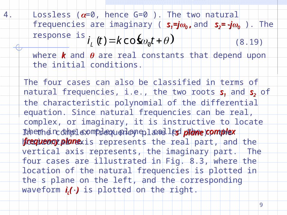
4. Lossless (=0, hence G=0 ). The two natural frequencies are imaginary ( ss11=j=j00 , , and s s22= -j= -j00 ). The response is

tktiL 0cos)(where kk and are real constants that depend upon the initial conditions.

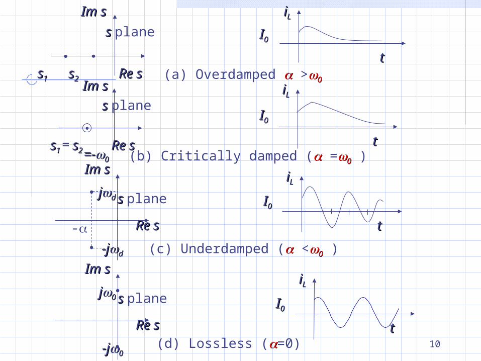
The four cases can also be classified in terms of natural frequencies, i.e., the two roots ss11 and ss22 of the characteristic polynomial of the differential equation. Since natural frequencies can be real, complex, or imaginary, it is instructive to locate them in the complex plane, called the complex frequency plane. complex frequency plane. In the complex frequency plane (ss planeplane), the horizontal axis represents the real part, and the vertical axis represents, the imaginary part. The four cases are illustrated in Fig. 8.3, where the location of the natural frequencies is plotted in the s plane on the left, and the corresponding waveform iiLL(()) is plotted on the right.

(8.19)

10

Im sIm s

s s plane

Re sRe sss11 ss22

iiLL

tt

II00

(a) Overdamped >00 Im sIm s

s s plane

Re sRe sss11 ss22==-=-00

iiLL

tt

II00

(b) Critically damped ( =00 ) Im sIm s

s s plane

Re sRe s

-j-jdd

jjdd

-

iiLL

tt

II00

Im sIm s

s s plane

Re sRe s

-j-j00

jj00

iiLL

tt

II00

(c) Underdamped ( <00 )

(d) Lossless (=0)

11

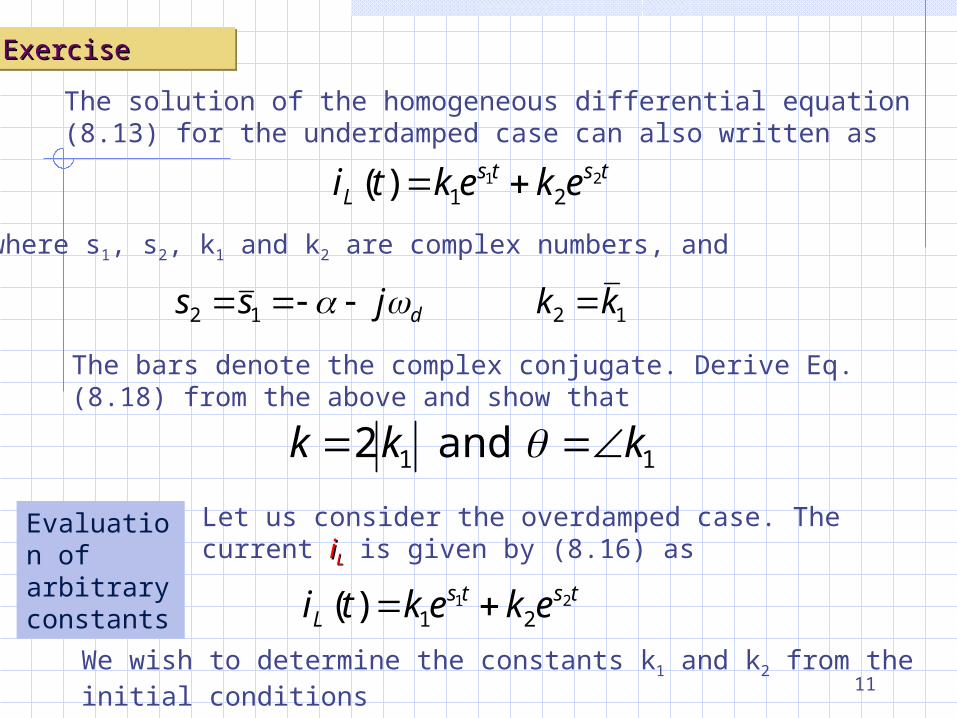
ExerciseExerciseExerciseExercise

The solution of the homogeneous differential equation (8.13) for the underdamped case can also written as

tstsL ekekti 21

21)(

where s1, s2, k1 and k2 are complex numbers, and

1212 kkjss d

The bars denote the complex conjugate. Derive Eq.(8.18) from the above and show that

11 and 2 kkk

Evaluation of arbitrary constants

Let us consider the overdamped case. The current iiLL is given by (8.16) as

tstsL ekekti 21

21)( We wish to determine the constants k1 and k2 from the initial conditions

12

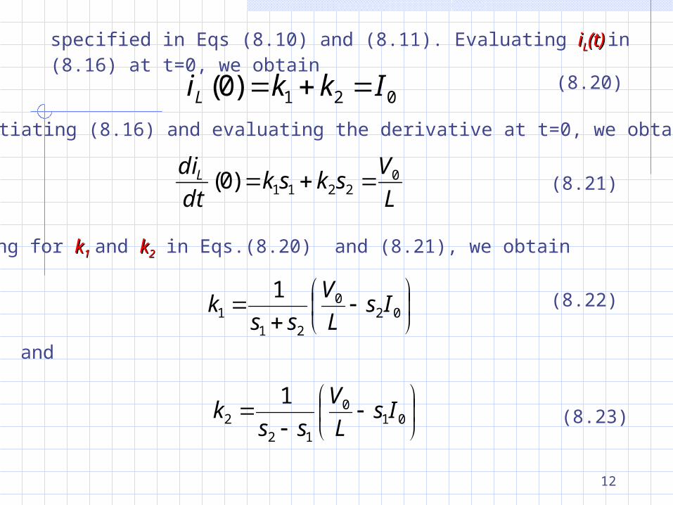
specified in Eqs (8.10) and (8.11). Evaluating iiLL(t)(t) in (8.16) at t=0, we obtain

021)0( IkkiL (8.20)

Differentiating (8.16) and evaluating the derivative at t=0, we obtain

L

Vsksk

dt

diL 02211)0( (8.21)

Solving for kk11 and kk22 in Eqs.(8.20) and (8.21), we obtain

02

0

211

1Is

L

V

ssk (8.22)

and

01

0

122

1Is

L

V

ssk (8.23)

13

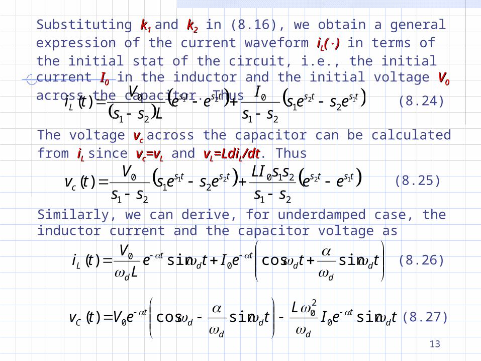
Substituting kk11 and kk22 in (8.16), we obtain a general expression of the current waveform iiLL(()) in terms of the initial stat of the circuit, i.e., the initial current II00 in the inductor and the initial voltage VV00 across the capacitor. Thus

tstststsL eses

ss

Iee

Lss

Vti 1221

2121

0

21

0)(

(8.24)

The voltage vvcc across the capacitor can be calculated from iiLL since vvcc=v=vLL and vvLL=Ldi=LdiLL/dt/dt. Thus

tstststsc ee

ss

ssLIeses

ss

Vtv 1221

21

21021

21

0)(

(8.25)

Similarly, we can derive, for underdamped case, the inductor current and the capacitor voltage as

tteIte

L

Vti d

dd

td

t

dL

sincossin)( 0

0 (8.26)

teIL

teVtv dt

dd

dd

tC

sinsincos)( 0

20

0

(8.27)

14

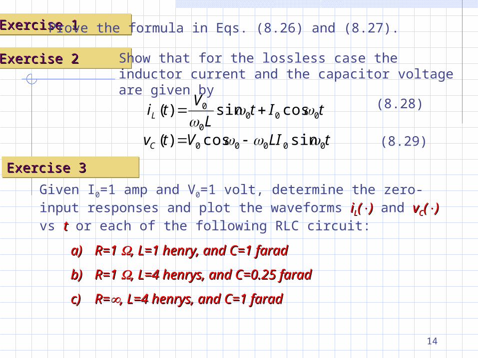
Exercise 1Exercise 1Exercise 1Exercise 1 Prove the formula in Eqs. (8.26) and (8.27).

Exercise 2Exercise 2Exercise 2Exercise 2 Show that for the lossless case the inductor current and the capacitor voltage are given by

tItL

VtiL 000

0

0 cossin)(

tLIVtvC 00000 sincos)(

(8.28)

(8.29)

Exercise 3Exercise 3Exercise 3Exercise 3

Given I0=1 amp and V0=1 volt, determine the zero-input responses and plot the waveforms iiLL(()) and vvCC(()) vs tt or each of the following RLC circuit:

a)a) R=1 R=1 , L=1 henry, and C=1 farad, L=1 henry, and C=1 farad

b)b) R=1 R=1 , L=4 henrys, and C=0.25 farad, L=4 henrys, and C=0.25 farad

c)c) R=R=, L=4 henrys, and C=1 farad, L=4 henrys, and C=1 farad

15

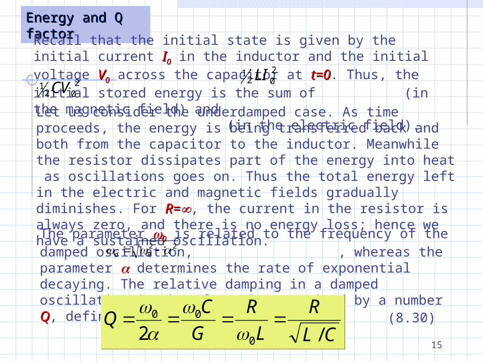
Energy and Q Energy and Q factorfactorRecall that the initial state is given by the initial current II00 in the inductor and the initial voltage VV00 across the capacitor at t=0t=0. Thus, the initial stored energy is the sum of (in the magnetic field) and (in the electric field).

202

1 LI2

021 CV

Let us consider the underdamped case. As time proceeds, the energy is being transferred back and both from the capacitor to the inductor. Meanwhile the resistor dissipates part of the energy into heat as oscillations goes on. Thus the total energy left in the electric and magnetic fields gradually diminishes. For R=R=, the current in the resistor is always zero, and there is no energy loss; hence we have a sustained oscillation.

The parameter 00 is related to the frequency of the damped oscillation, , whereas the parameter determines the rate of exponential decaying. The relative damping in a damped oscillation is the often characterized by a number QQ, defined by

220 d

CL

R

L

R

G

CQ

/2 0

00

CL

R

L

R

G

CQ

/2 0

00

(8.30)

16

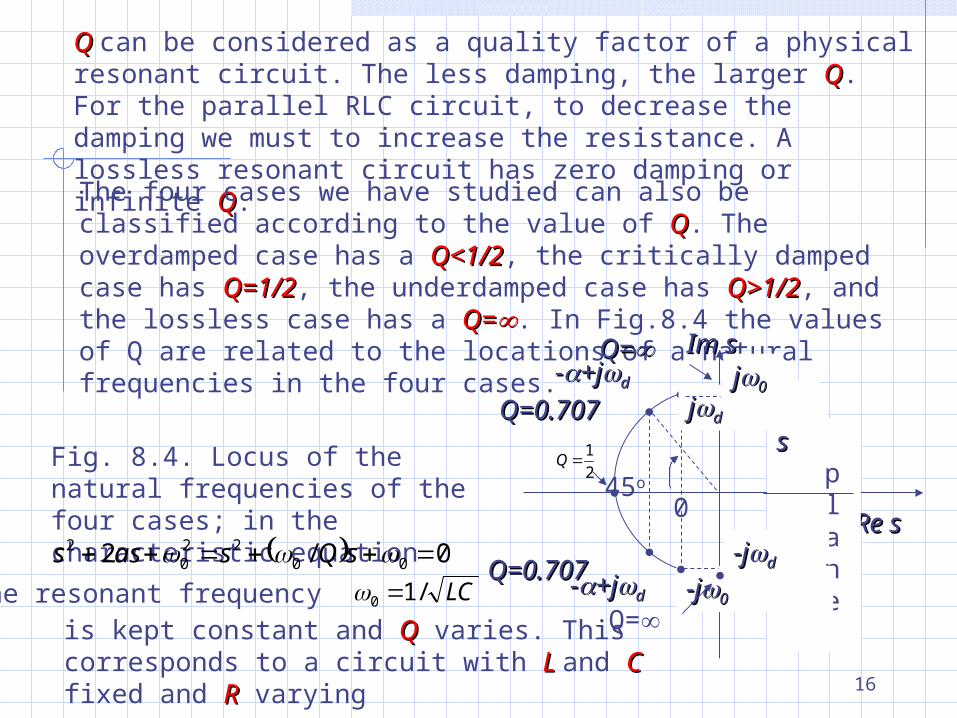
Q Q can be considered as a quality factor of a physical resonant circuit. The less damping, the larger QQ. For the parallel RLC circuit, to decrease the damping we must to increase the resistance. A lossless resonant circuit has zero damping or infinite QQ.The four cases we have studied can also be classified according to the value of QQ. The overdamped case has a Q<1/2Q<1/2, the critically damped case has Q=1/2Q=1/2, the underdamped case has Q>1/2Q>1/2, and the lossless case has a Q=Q=. In Fig.8.4 the values of Q are related to the locations of a natural frequencies in the four cases.

Re sRe s

Im sIm s

s s plane

-j-j00

0

-j-jdd

Q=

jjdd

jj00

Q=Q=--+j+jdd

Q=0.707Q=0.707

2

1Q

Q=0.707Q=0.707--+j+jdd

45oFig. 8.4. Locus of the natural frequencies of the four cases; in the characteristic equation

0/2 0022

02 sQsass

The resonant frequency LC/10 is kept constant and QQ varies. This corresponds to a circuit with L L and CC fixed and RR varying

17

Linear time invariant Linear time invariant RLCRLC-circuits, zero-state response-circuits, zero-state response

Let us continue with the same linear time-invariant parallel RLC circuit to illustrate the computation and properties of the zero state responseBy zero-state response we mean the response of a circuit due to an input applied at some arbitrary time t0 subject to the condition that the circuit is in the zero state at t0-.

iicc ++vvRR

--

+vc-

iiRR iiLL

+vL-iiss

Fig. 8.5 Parallel RLC circuit with current source as input

KCL for the circuit in Fig. 8.5 gives

sLRC iiii (8.31)

Following the same procedure that in previous section we obtain the network equation in terms of inductor current iiLL. Thus

0 )(2

2

ttiidt

diGL

dt

idLC sL

LL (8.32)

and

18

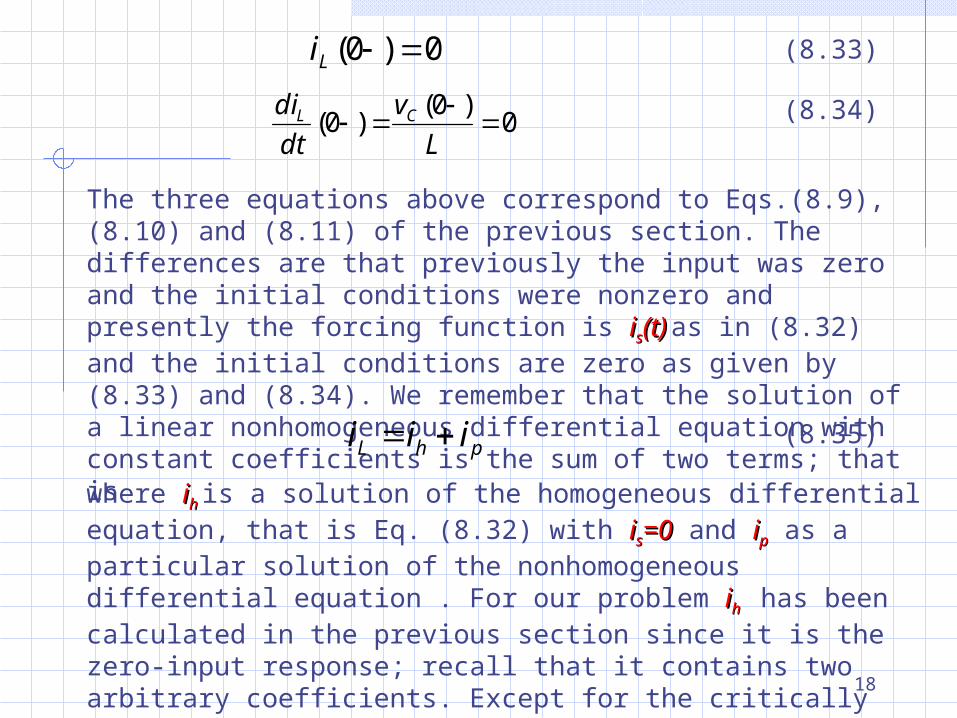
0)0( Li (8.33)

0)0(

)0(

L

v

dt

di CL (8.34)

The three equations above correspond to Eqs.(8.9), (8.10) and (8.11) of the previous section. The differences are that previously the input was zero and the initial conditions were nonzero and presently the forcing function is iiss(t)(t) as in (8.32) and the initial conditions are zero as given by (8.33) and (8.34). We remember that the solution of a linear nonhomogeneous differential equation with constant coefficients is the sum of two terms; that is

phL iii (8.35)

where iih h is a solution of the homogeneous differential equation, that is Eq. (8.32) with iiss=0=0 and iipp as a particular solution of the nonhomogeneous differential equation . For our problem iih h has been calculated in the previous section since it is the zero-input response; recall that it contains two arbitrary coefficients. Except for the critically damped case, iih h can be written in the form

19

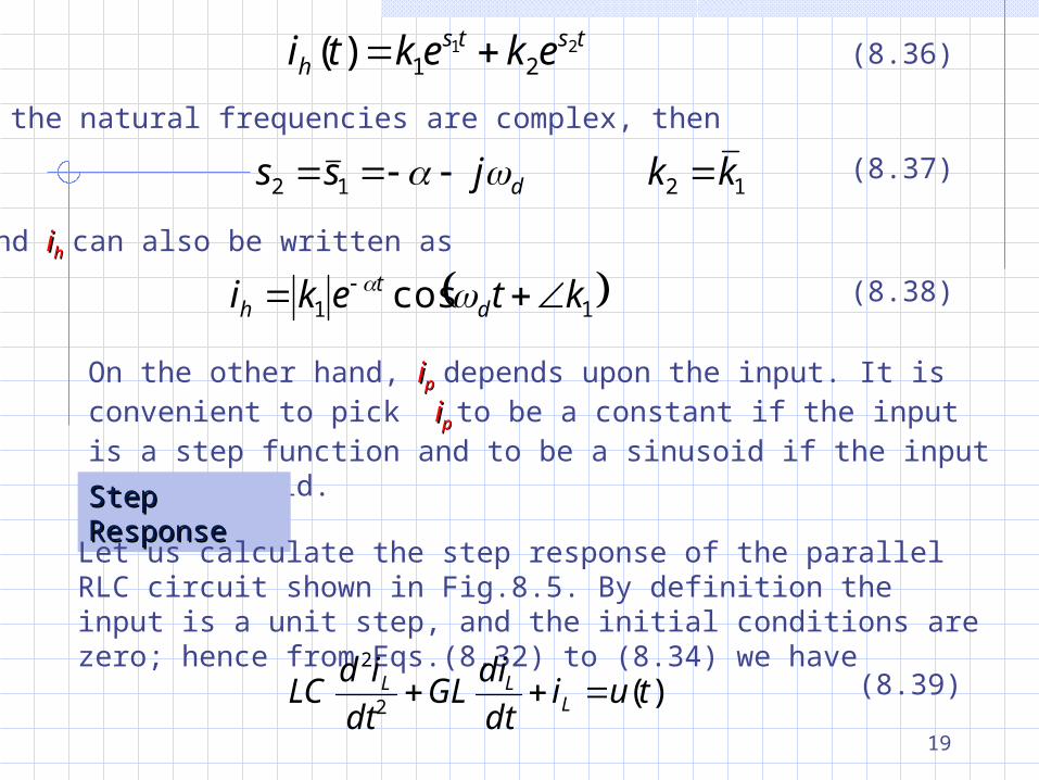
tstsh ekekti 21

21)( (8.36)

If the natural frequencies are complex, then

1212 kkjss d (8.37)

and iih h can also be written as

11 cos kteki dt

h (8.38)

On the other hand, iip p depends upon the input. It is convenient to pick iip p to be a constant if the input is a step function and to be a sinusoid if the input is a sinusoid.

Step Step ResponseResponse

Let us calculate the step response of the parallel RLC circuit shown in Fig.8.5. By definition the input is a unit step, and the initial conditions are zero; hence from Eqs.(8.32) to (8.34) we have

)(2

2

tuidt

diGL

dt

idLC L

LL (8.39)

20

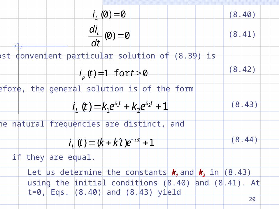
0)0( Li (8.40)

0)0( dt

diL (8.41)

The most convenient particular solution of (8.39) is

0for 1)( ttip(8.42)

Therefore, the general solution is of the form

1)( 2121 tsts

L ekekti (8.43)

if the natural frequencies are distinct, and

1)()( tL etkkti (8.44)

if they are equal.

Let us determine the constants kk11 and kk22 in (8.43) using the initial conditions (8.40) and (8.41). At t=0, Eqs. (8.40) and (8.43) yield

21

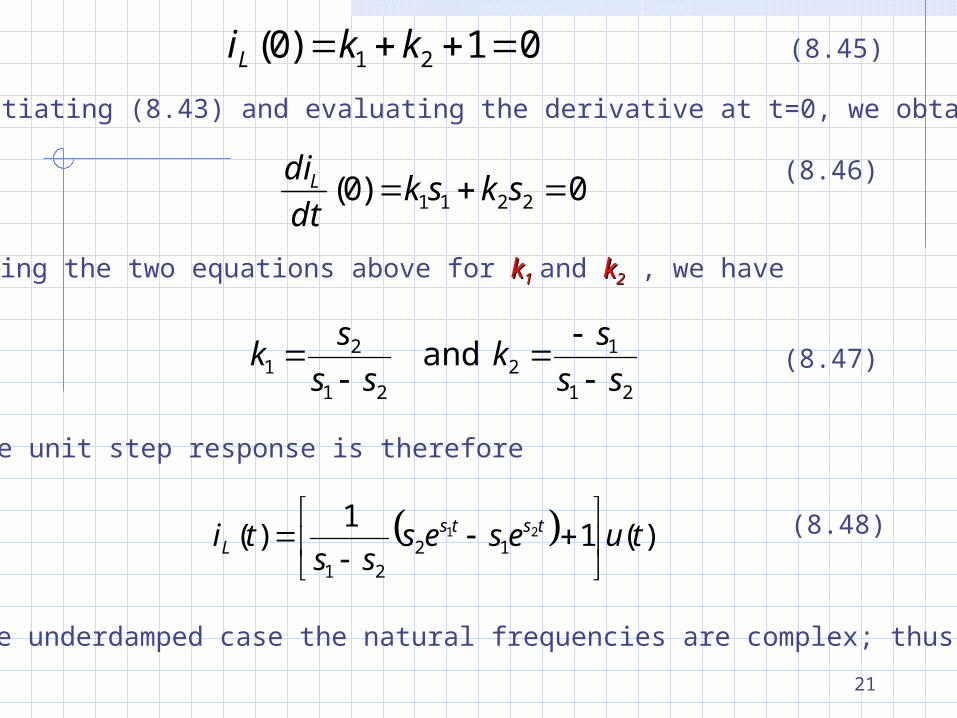
01)0( 21 kkiL (8.45)

Differentiating (8.43) and evaluating the derivative at t=0, we obtain

0)0( 2211 skskdt

diL (8.46)

Solving the two equations above for kk11 and kk22 , we have

21

12

21

21 and

ss

sk

ss

sk

(8.47)

The unit step response is therefore

)(11

)( 2112

21

tuesesss

ti tstsL

(8.48)

In the underdamped case the natural frequencies are complex; thus,

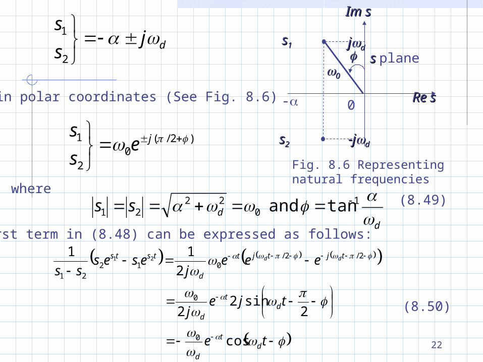
22

djs

s

2

1

or in polar coordinates (See Fig. 8.6)

)2/(0

2

1 je

s

s

Im sIm s

s s plane

Re sRe s

-j-jdd

jjddss11

ss22

-

00

0

Fig. 8.6 Representing natural frequencies

where

ddss

1

022

21 tan and (8.49)

The first term in (8.48) can be expressed as follows:

te

tjej

eeej

esesss

dt

d

dt

d

tjtjt

d

tsts dd

cos

2sin2

2

2

11

0

0

2/2/012

21

21

(8.50)

23

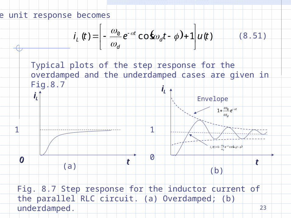
)(1cos)( 0 tuteti dt

dL

The unit response becomes

(8.51)

teti d

t

dL cos1)( 0

t

d

e

01

Envelope

iiLL

1

0tt

(b)

Fig. 8.7 Step response for the inductor current of the parallel RLC circuit. (a) Overdamped; (b) underdamped.

Typical plots of the step response for the overdamped and the underdamped cases are given in Fig.8.7

00 tt

1

(a)

iiLL

24

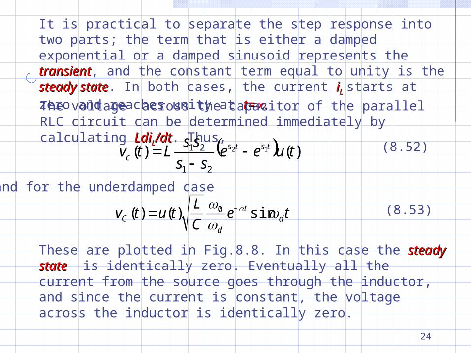
It is practical to separate the step response into two parts; the term that is either a damped exponential or a damped sinusoid represents the transienttransient, and the constant term equal to unity is the steady statesteady state. In both cases, the current iiLL starts at zero and reaches unity at t=t=. . The voltage across the capacitor of the parallel RLC circuit can be determined immediately by calculating LdiLdiLL/dt/dt. Thus,

)()( 12

21

21 tueess

ssLtv tsts

c

(8.52)

and for the underdamped case

teC

Ltutv d

t

dC

sin)()( 0 (8.53)

These are plotted in Fig.8.8. In this case the steady statesteady state is identically zero. Eventually all the current from the source goes through the inductor, and since the current is constant, the voltage across the inductor is identically zero.

25

vvCC

tt

t

d

eC

L

0

teC

Ltv d

t

dC

sin)( 0

d

d2

slopeC

1

00 tt(a)

vvCC

slopeC

1(b)

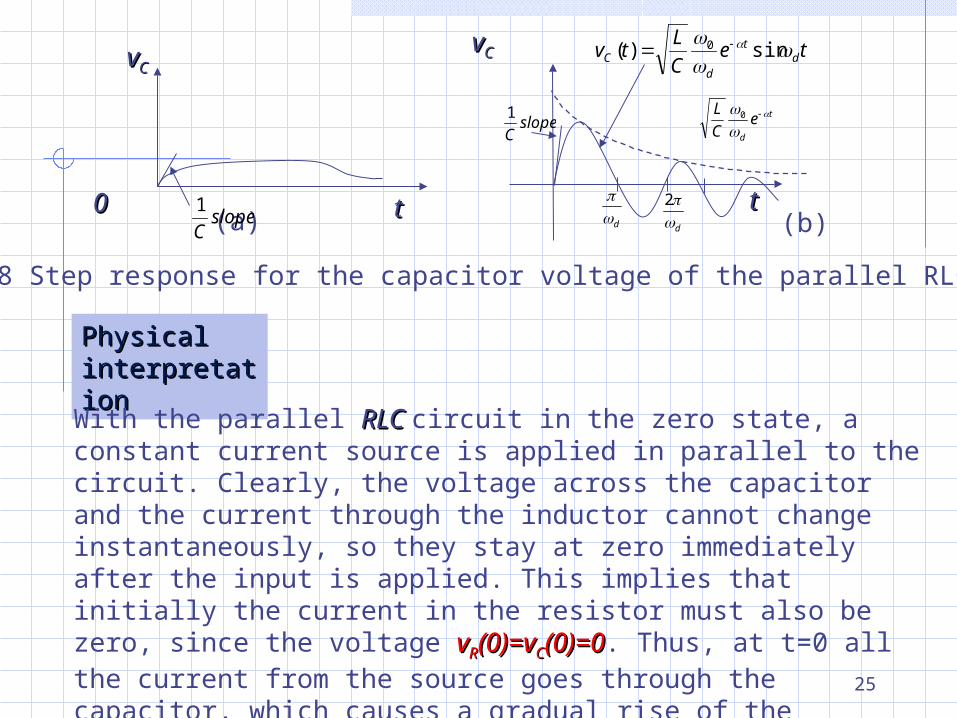
Fig.8.8 Step response for the capacitor voltage of the parallel RLC circuit

Physical Physical interpretatiointerpretationn

With the parallel RLC RLC circuit in the zero state, a constant current source is applied in parallel to the circuit. Clearly, the voltage across the capacitor and the current through the inductor cannot change instantaneously, so they stay at zero immediately after the input is applied. This implies that initially the current in the resistor must also be zero, since the voltage vvRR(0)=v(0)=vCC(0)=0(0)=0. Thus, at t=0 all the current from the source goes through the capacitor, which causes a gradual rise of the voltage. At t=0+t=0+ the capacitor acts as a short circuit to a the capacitor acts as a short circuit to a suddenly applied finite constant current sourcesuddenly applied finite constant current source.

26

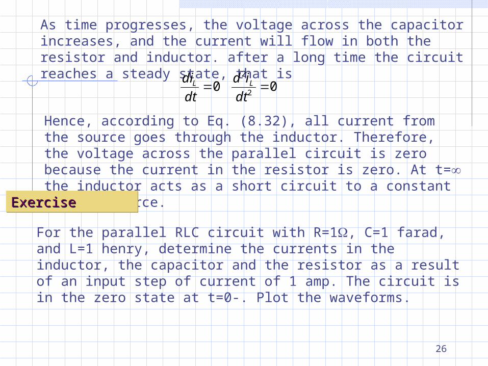
As time progresses, the voltage across the capacitor increases, and the current will flow in both the resistor and inductor. after a long time the circuit reaches a steady state, that is

0 02

2

dt

id

dt

di LL

Hence, according to Eq. (8.32), all current from the source goes through the inductor. Therefore, the voltage across the parallel circuit is zero because the current in the resistor is zero. At t= the inductor acts as a short circuit to a constant current source.

Exercise Exercise Exercise Exercise

For the parallel RLC circuit with R=1, C=1 farad, and L=1 henry, determine the currents in the inductor, the capacitor and the resistor as a result of an input step of current of 1 amp. The circuit is in the zero state at t=0-. Plot the waveforms.

27

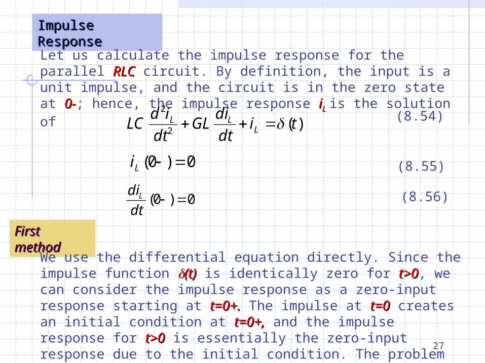
Impulse Impulse ResponseResponseLet us calculate the impulse response for the parallel RLCRLC circuit. By definition, the input is a unit impulse, and the circuit is in the zero state at 0-0-; hence, the impulse response iiLL is the solution of

)(2

2

tidt

diGL

dt

idLC L

LL (8.54)

0)0( Li

0)0( dt

diL

(8.55)

(8.56)

First methodFirst method

We use the differential equation directly. Since the impulse function (t)(t) is identically zero for t>0t>0, we can consider the impulse response as a zero-input response starting at t=0+.t=0+. The impulse at t=0t=0 creates an initial condition at t=0+,t=0+, and the impulse response for t>0t>0 is essentially the zero-input response due to the initial condition. The problem then is to determine this initial condition.

28

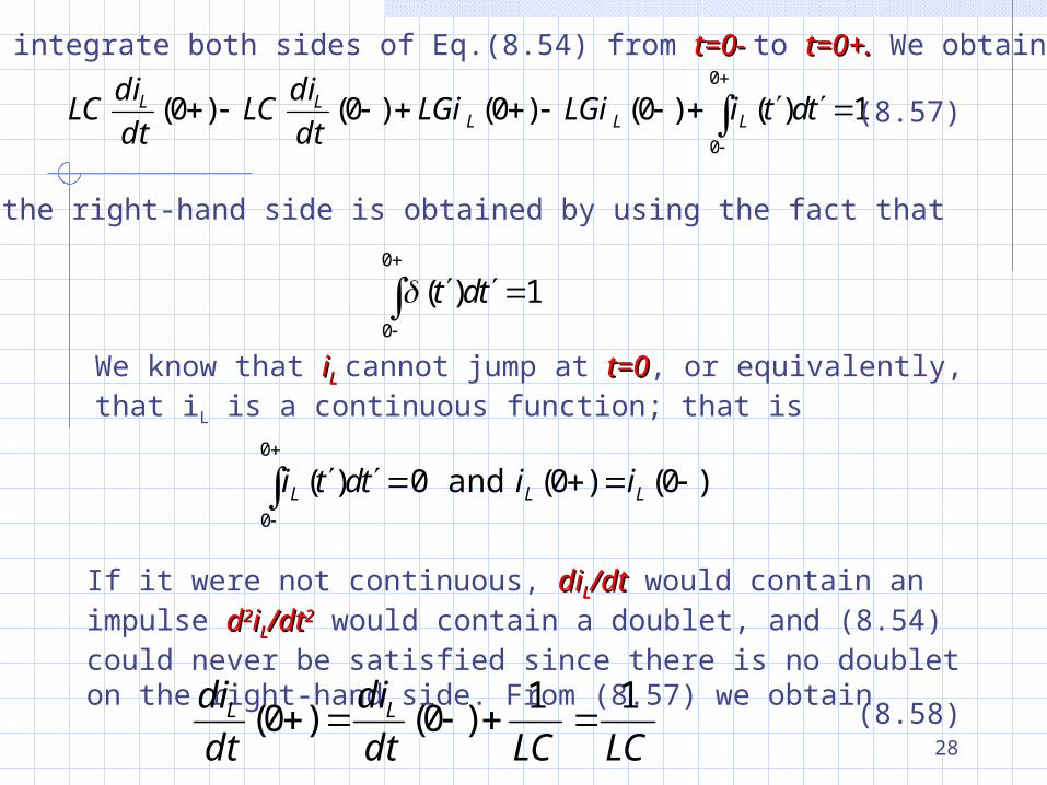
Let us integrate both sides of Eq.(8.54) from t=0- t=0- to t=0+.t=0+. We obtain

1)()0()0()0()0(0

0

tdtiLGiLGidt

diLC

dt

diLC LLL

LL (8.57)

where the right-hand side is obtained by using the fact that

1)(0

0

tdt

We know that iiLL cannot jump at t=0t=0, or equivalently, that iL is a continuous function; that is

)0()0( and 0)(0

0

LLL iitdti

If it were not continuous, didiLL/dt/dt would contain an impulse dd22iiLL/dt/dt22 would contain a doublet, and (8.54) could never be satisfied since there is no doublet on the right-hand side. From (8.57) we obtain

LCLCdt

di

dt

di LL 11)0()0( (8.58)

29

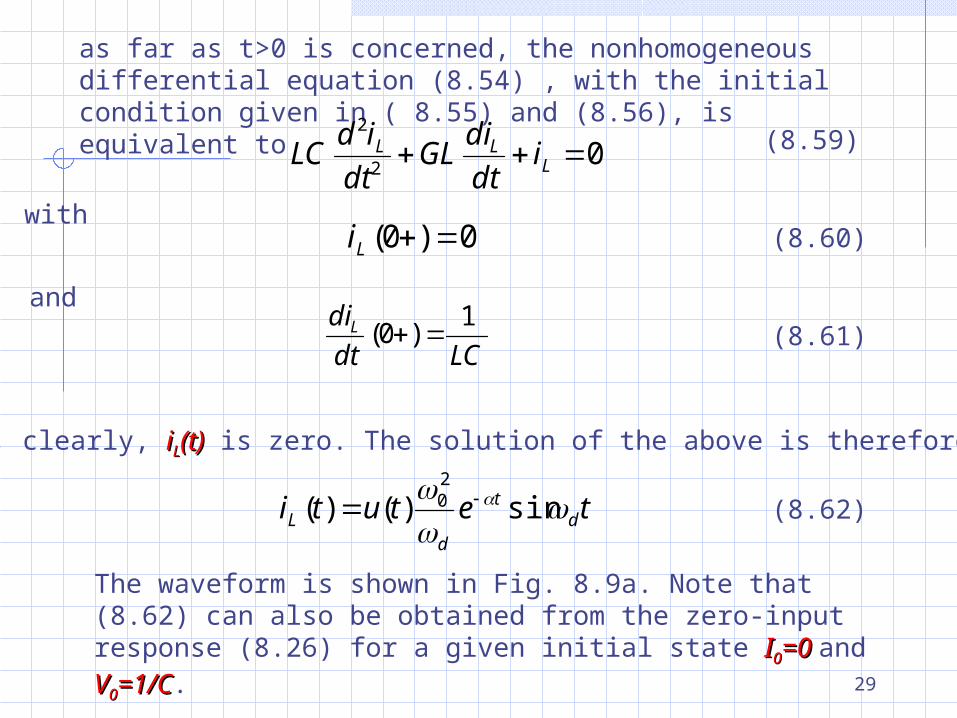
as far as t>0 is concerned, the nonhomogeneous differential equation (8.54) , with the initial condition given in ( 8.55) and (8.56), is equivalent to

02

2

LLL i

dt

diGL

dt

idLC (8.59)

with0)0( Li

LCdt

diL 1)0(

and

(8.60)

(8.61)

For tt00, clearly, iiLL(t)(t) is zero. The solution of the above is therefore

tetuti dt

dL

sin)()(

20

The waveform is shown in Fig. 8.9a. Note that (8.62) can also be obtained from the zero-input response (8.26) for a given initial state II00=0 =0 and VV00=1/C=1/C.

(8.62)

30

iiLL

tt

t

d

e

2

0

d

d2

teti dt

dL

sin)(

20

EnvelopeEnvelope

vvCC

tt

t

d

eC

L

2

0

te

C

Ltv d

t

dC cos)(

20

EnvelopeEnvelope

d

t

2

2

C

1

(a) (b)

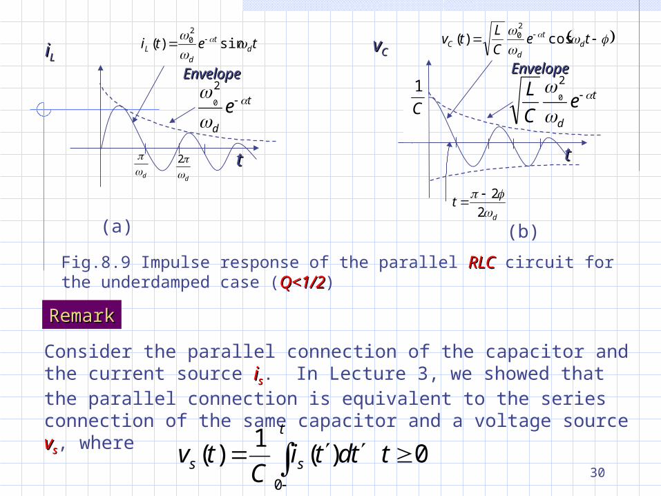
Fig.8.9 Impulse response of the parallel RLCRLC circuit for the underdamped case (Q<1/2Q<1/2)

RemarkRemark

Consider the parallel connection of the capacitor and the current source iiss. In Lecture 3, we showed that the parallel connection is equivalent to the series connection of the same capacitor and a voltage source vvss, where

0 )(1

)(0

ttdtiC

tvt

ss

31

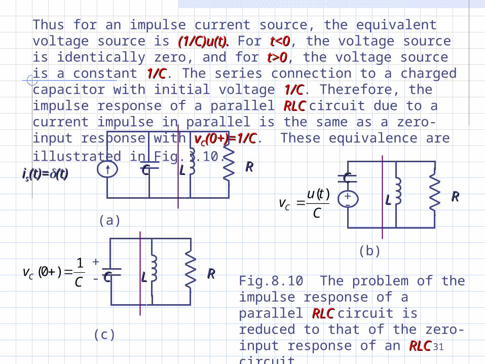
Thus for an impulse current source, the equivalent voltage source is (1/C)u(t).(1/C)u(t). For t<0t<0, the voltage source is identically zero, and for t>0t>0, the voltage source is a constant 1/C1/C. The series connection to a charged capacitor with initial voltage 1/C1/C. Therefore, the impulse response of a parallel RLC RLC circuit due to a current impulse in parallel is the same as a zero-input response with vvCC(0+)=1/C(0+)=1/C. These equivalence are illustrated in Fig.8.10.

iiss(t)=(t)=(t)(t) RRCC LL

(a)

RRCC

LLC

tuvC

)( +

-

(b)

RRCC LLCvC

1)0(

+-

(c)

Fig.8.10 The problem of the impulse response of a parallel RLC RLC circuit is reduced to that of the zero-input response of an RLCRLC circuit

32

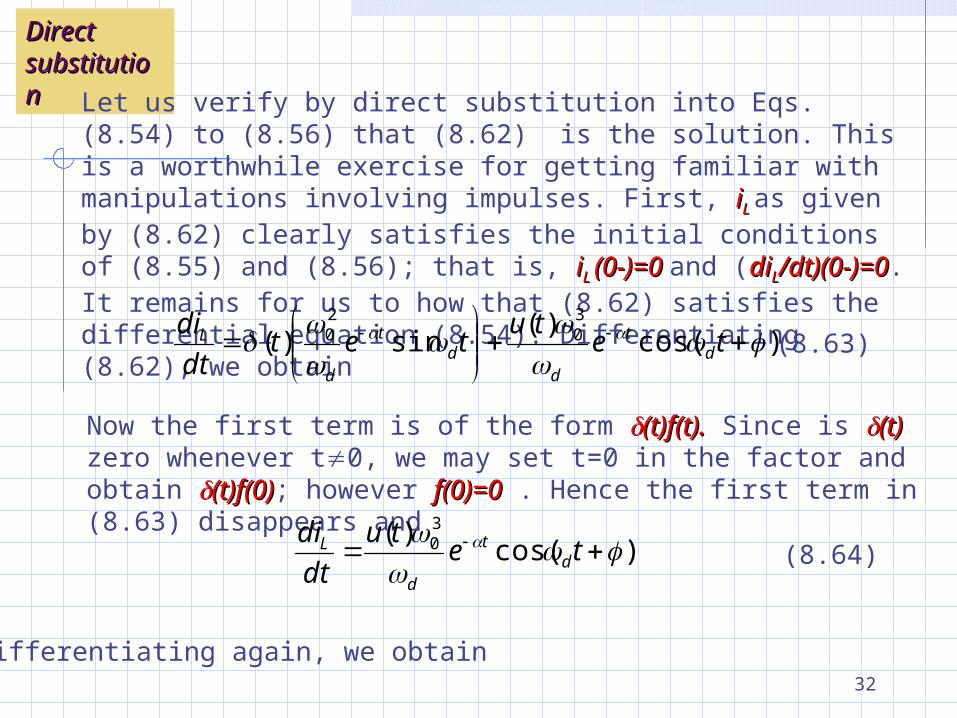
Direct Direct substitutionsubstitution

Let us verify by direct substitution into Eqs.(8.54) to (8.56) that (8.62) is the solution. This is a worthwhile exercise for getting familiar with manipulations involving impulses. First, iiL L as given by (8.62) clearly satisfies the initial conditions of (8.55) and (8.56); that is, iiL L (0-)=0 (0-)=0 and (didiLL/dt)(0-)=0/dt)(0-)=0. It remains for us to how that (8.62) satisfies the differential equation (8.54). Differentiating (8.62), we obtain

)cos()(

sin)(30

20

te

tutet

dt

did

t

dd

t

d

L (8.63)

Now the first term is of the form (t)f(t).(t)f(t). Since is (t) (t) zero whenever t0, we may set t=0 in the factor and obtain (t)f(0)(t)f(0); however f(0)=0f(0)=0 . Hence the first term in (8.63) disappears and

)cos()( 3

0

tetu

dt

did

t

d

L (8.64)

Differentiating again, we obtain

33

sin)cos(cos)sin()()(

)2sin()(cos)(

402

0

40

30

2

2

ttetut

tetutdt

id

ddt

d

dt

dd

L

(8.65)

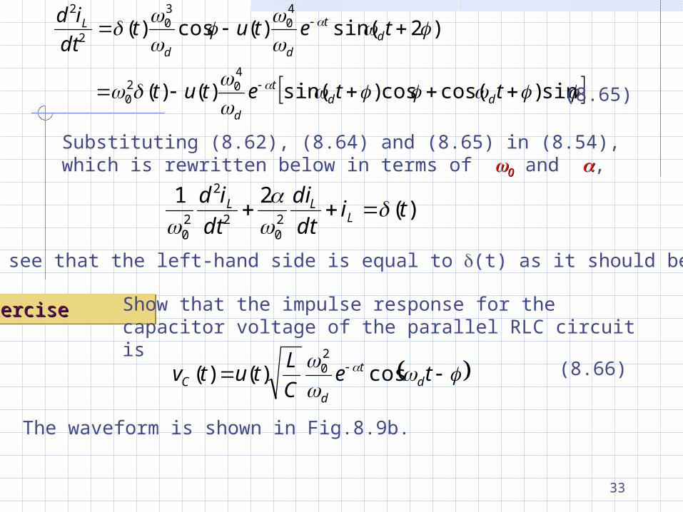
Substituting (8.62), (8.64) and (8.65) in (8.54), which is rewritten below in terms of 00 and ,

)(21

20

2

2

20

tidt

di

dt

idL

LL

we shall see that the left-hand side is equal to (t) as it should be.

Exercise Exercise Exercise Exercise Show that the impulse response for the capacitor voltage of the parallel RLC circuit is

te

C

Ltutv d

t

dC cos)()(

20 (8.66)

The waveform is shown in Fig.8.9b.

34

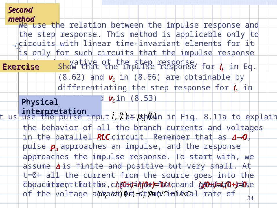
Second methodSecond method

We use the relation between the impulse response and the step response. This method is applicable only to circuits with linear time-invariant elements for it is only for such circuits that the impulse response is the derivative of the step response.

ExerciseExercise Show that the impulse response for iiL L in Eq.(8.62) and vvCC in (8.66) are obtainable by differentiating the step response for iiL L in (8.51) and vvC C in (8.53)

Physical Physical interpretationinterpretation

Let us use the pulse input )()( tptis as shown in Fig. 8.11a to explain the behavior of all the branch currents and voltages in the parallel RLC RLC circuit. Remember that as 00, pulse pp

approaches an impulse, and the response approaches the impulse response. To start with, we assume is finite and positive but very small. At t=0+ all the current from the source goes into the capacitor; that is, iiCC(0+)=i(0+)=iss(0+)=1/(0+)=1/, and iiRR(0+)=i(0+)=iLL(0+)=0(0+)=0.

CCidtdv CC /1/)0()0)(/(The current in the capacitor forces a gradual rise of the voltage across it at an initial rate of

35

tt

iiss= p= p1

(a)0

tt

vvCC

C

1

0

CSlope

1

(b)

tt

1

dt

dvCi C

C

(c)tt

RC

1

R

vi CR

(d)tt

LC2

t

CL tdtvL

i0

)(1

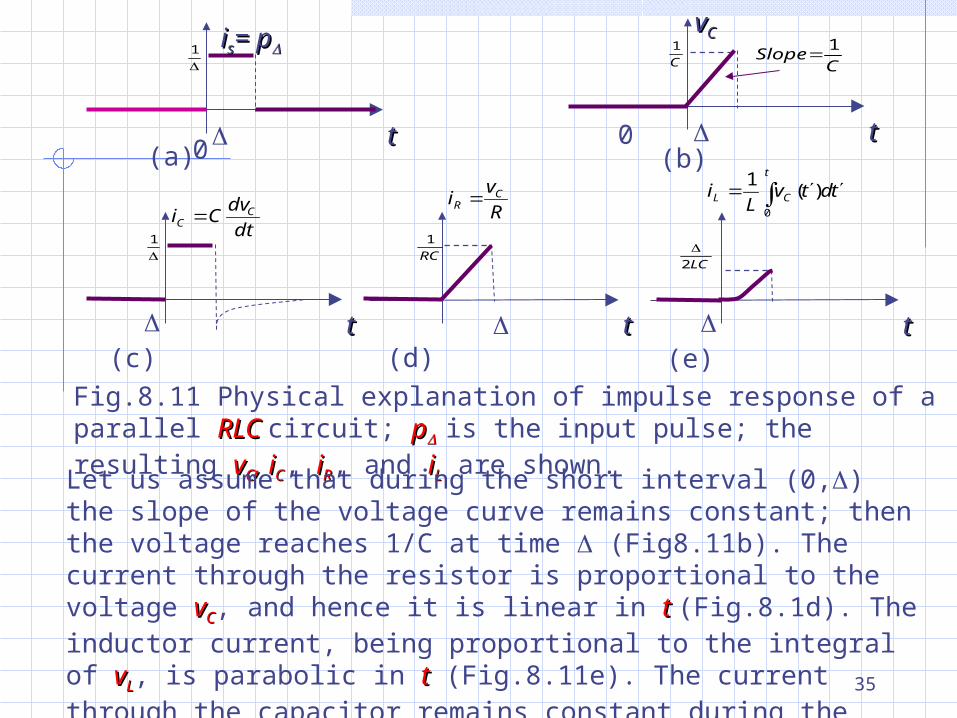
(e)Fig.8.11 Physical explanation of impulse response of a parallel RLC RLC circuit; pp is the input pulse; the resulting vvCC, i, iCC, iiRR, and iiLL are shown.Let us assume that during the short interval (0,) the slope of the voltage curve remains constant; then the voltage reaches 1/C at time (Fig8.11b). The current through the resistor is proportional to the voltage vvCC, and hence it is linear in t t (Fig.8.1d). The inductor current, being proportional to the integral of vvLL, is parabolic in tt (Fig.8.11e). The current through the capacitor remains constant during the interval, as shown in Fig. 8.11c.

36

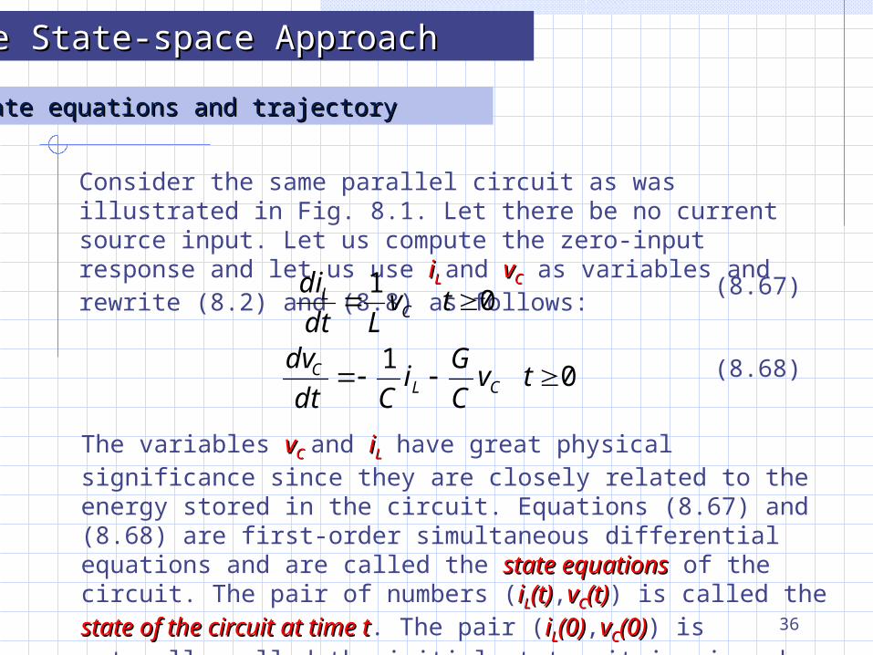
The State-space ApproachThe State-space Approach

State equations and trajectoryState equations and trajectory

Consider the same parallel circuit as was illustrated in Fig. 8.1. Let there be no current source input. Let us compute the zero-input response and let us use iiL L and vvCC as variables and rewrite (8.2) and (8.8) as follows:

0 1

tvLdt

diC

L

0 1

tvC

Gi

Cdt

dvCL

C

(8.67)

(8.68)

The variables vvCC and iiLL have great physical significance since they are closely related to the energy stored in the circuit. Equations (8.67) and (8.68) are first-order simultaneous differential equations and are called the state equationsstate equations of the circuit. The pair of numbers (iiLL(t)(t),vvCC(t)(t)) is called the state of state of the circuit at time tthe circuit at time t. The pair (iiLL(0)(0),vvCC(0)(0)) is naturally called the initial state; it is given by initial conditions

37

0

0

)0(

)0(

Vv

Ii

C

L

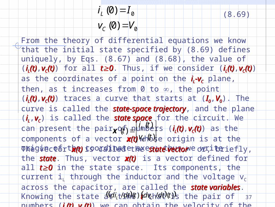
(8.69)

From the theory of differential equations we know that the initial state specified by (8.69) defines uniquely, by Eqs. (8.67) and (8.68), the value of (iiLL(t)(t),vvCC(t)(t)) for all tt00. Thus, if we consider (iiLL(t)(t),vvCC(t)(t)) as the coordinates of a point on the iiLL-v-vCC plane, then, as t increases from 0 to , the point (iiLL(t)(t),vvCC(t)(t)) traces a curve that starts at (II00,VV00). The curve is called the state-space trajectorystate-space trajectory, and the plane (iiLL,vvCC) is called the state state spacespace for the circuit. We can present the pair of numbers (iiLL(t)(t),vvCC(t)(t)) as the components of a vector xx(t) (t) whose origin is at the origin of the coordinate axes; thus we write

)(

)()(

tv

tit

C

Lx

The vector xx(t) (t) is called the state vectorstate vector or, briefly, the statestate. Thus, vector xx(t) (t) is a vector defined for all tt00 in the state space. Its components, the current iL through the inductor and the voltage vC across the capacitor, are called the state state variablesvariables. Knowing the state at time tt that is the pair of numbers (iiLL(t)(t),vvCC(t)(t)) we can obtain the velocity of the trajectory from the state equations.

)(/),(/ tdtdvtdtdi CL

38

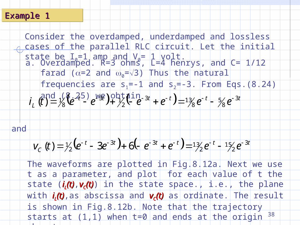
Example 1Example 1Example 1Example 1

Consider the overdamped, underdamped and lossless cases of the parallel RLC circuit. Let the initial state be I0=1 amp and V0= 1 volt.a. Overdamped. R=3 ohms, L=4 henrys, and C= 1/12 farad

(=2 and 0=3) Thus the natural frequencies are s1=-1 and s2=-3. From Eqs.(8.24) and (8.25) we obtain

ttttttL eeeeeeti 3

85

8133

213

81)(

and

ttttttC eeeeeetv 3

215

21333

21 63)(

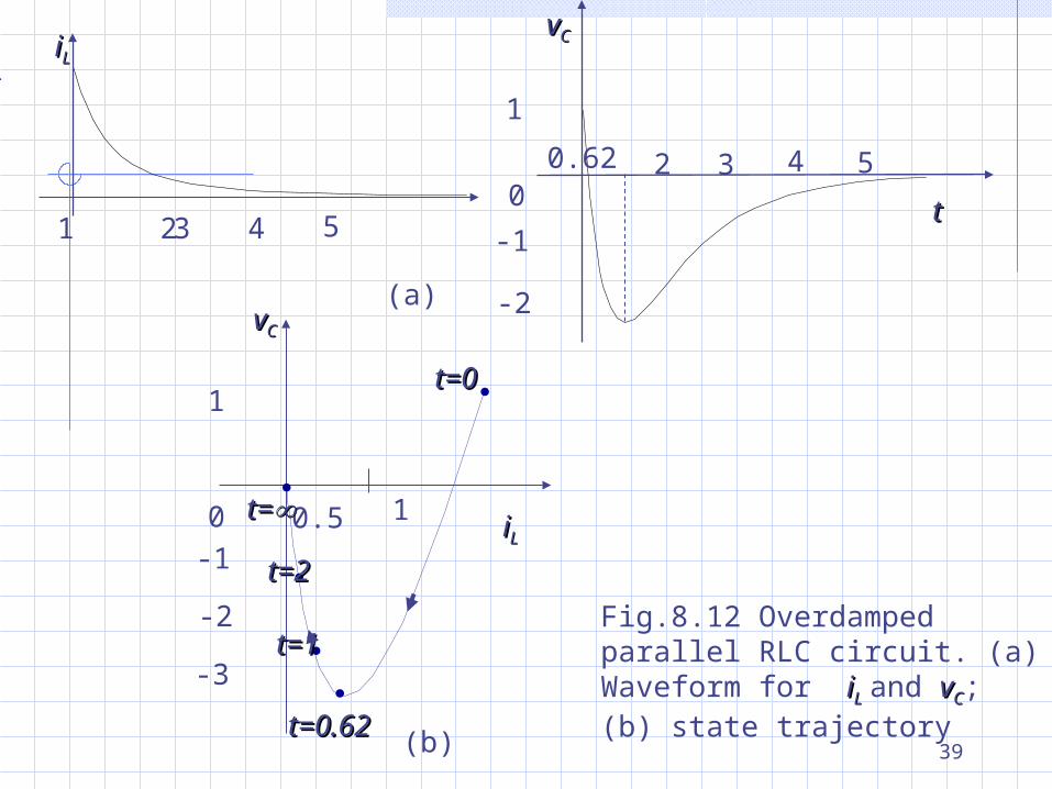
The waveforms are plotted in Fig.8.12a. Next we use t as a parameter, and plot for each value of t the state (iiLL(t)(t),vvCC(t)(t)) in the state space., i.e., the plane with iiLL(t)(t),as abscissa and vvCC(t)(t) as ordinate. The result is shown in Fig.8.12b. Note that the trajectory starts at (1,1) when t=0 and ends at the origin when t=.

39

iiLL

vvCC

10.5

t=0t=0

0-1

-2

-3

t=0.62t=0.62

t=1t=1

t=2t=2

t=t=

1

(b)

1

0

-1

-2

vvCC

tt

0.62 5432

(a)

1iiLL

54320 1

Fig.8.12 Overdamped parallel RLC circuit. (a) Waveform for iiLL and vvCC; (b) state trajectory

40

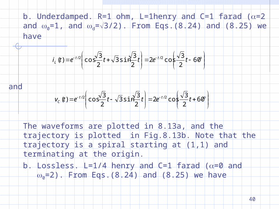
b. Underdamped. R=1 ohm, L=1henry and C=1 farad (=2 and 0=1, and d=3/2). From Eqs.(8.24) and (8.25) we have

ott

L tetteti 602

3cos2

2

3sin3

2

3cos)( 2/2/

and

ott

C tettetv 602

3cos2

2

3sin3

2

3cos)( 2/2/

The waveforms are plotted in 8.13a, and the trajectory is plotted in Fig.8.13b. Note that the trajectory is a spiral starting at (1,1) and terminating at the origin.

b. Lossless. L=1/4 henry and C=1 farad (=0 and 0=2). From Eqs.(8.24) and (8.25) we have

41

iiLL

54320 1

1

vvCC

54

32

0

1

1

iiLL

vvCC

1

t=0t=01

0

Fig.8.13 Underdamped parallel RLC circuit. Overdamped parallel RLC circuit. (a) Waveform for iiLL and vvCC; (b) state trajectory

(b)

(a)

42

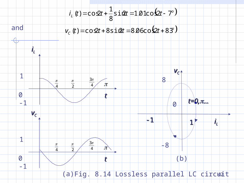
oL tttti 72cos01.12sin

8

12cos)(

and oC ttttv 832cos06.82sin82cos)(

iiLL

0

4

2

4

3

1

-1tt

vvCC

0

4

2

4

3

1

-1tt

iiLL

vvCC

t=0,t=0,……0

-8

8

-1-1 11

(b)

(a) Fig. 8.14 Lossless parallel LC circuit

43

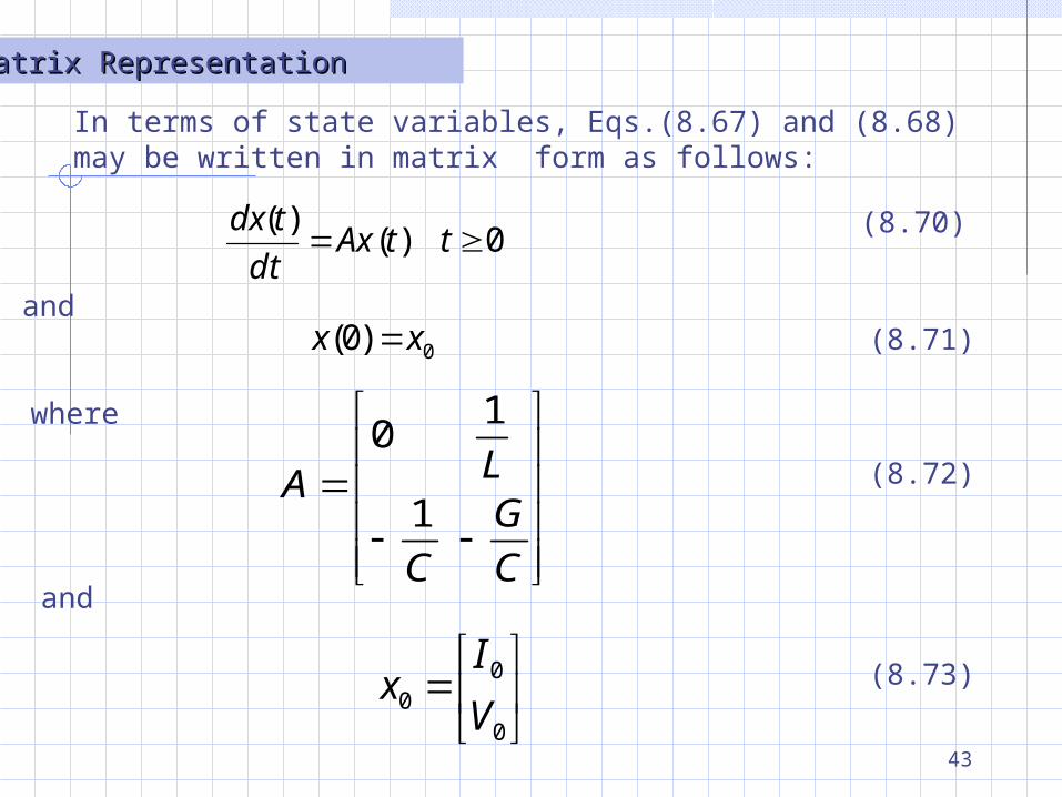
Matrix RepresentationMatrix Representation

In terms of state variables, Eqs.(8.67) and (8.68) may be written in matrix form as follows:

0 )()(

ttAxdt

tdx

and

(8.70)

0)0( xx (8.71)

where

C

G

C

LA

1

1 0

and

0

00 V

Ix

(8.72)

(8.73)

44

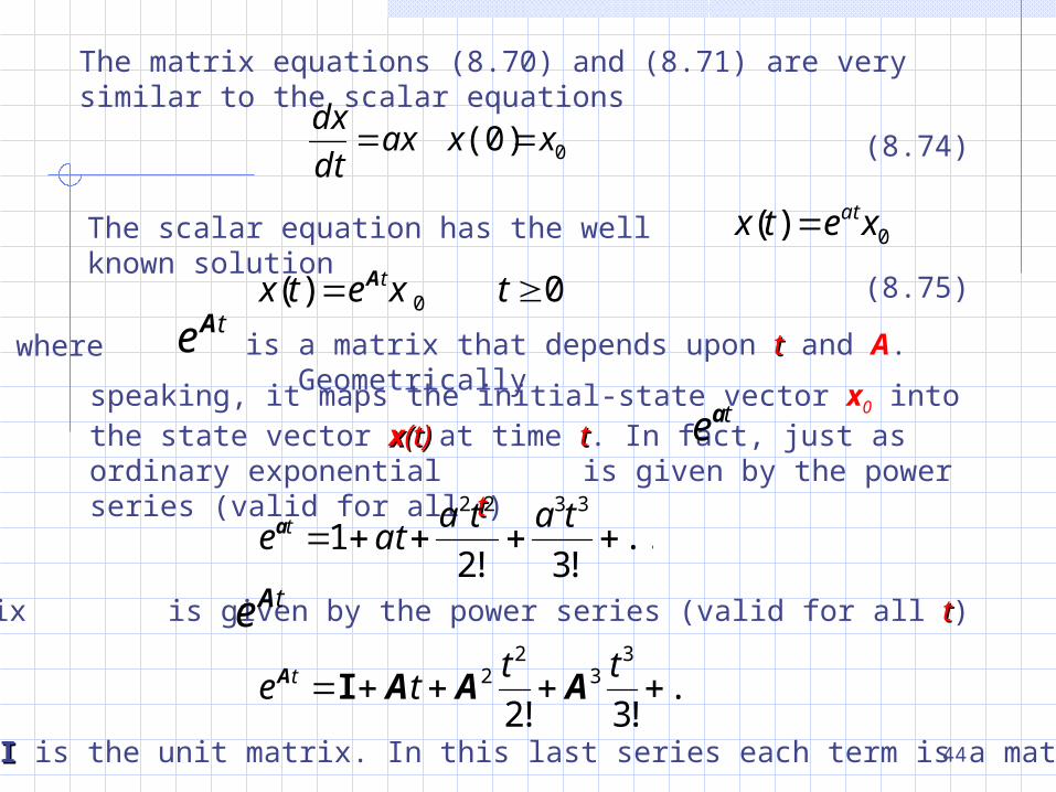
The matrix equations (8.70) and (8.71) are very similar to the scalar equations

0(0) xxaxdt

dx (8.74)

The scalar equation has the well known solution

0)( xetx at

(8.75)0 )( 0 tetx txA

where teA is a matrix that depends upon tt and A.

Geometrically speaking, it maps the initial-state vector x0 into the state vector xx(t)(t) at time tt. In fact, just as ordinary exponential is given by the power series (valid for all tt)

tea

...!3!2

13322

tata

ate ta

the matrix is given by the power series (valid for all tt) teA

...!3!2

33

22

ttte t AAAA I

where I I is the unit matrix. In this last series each term is a matrix; hence

45

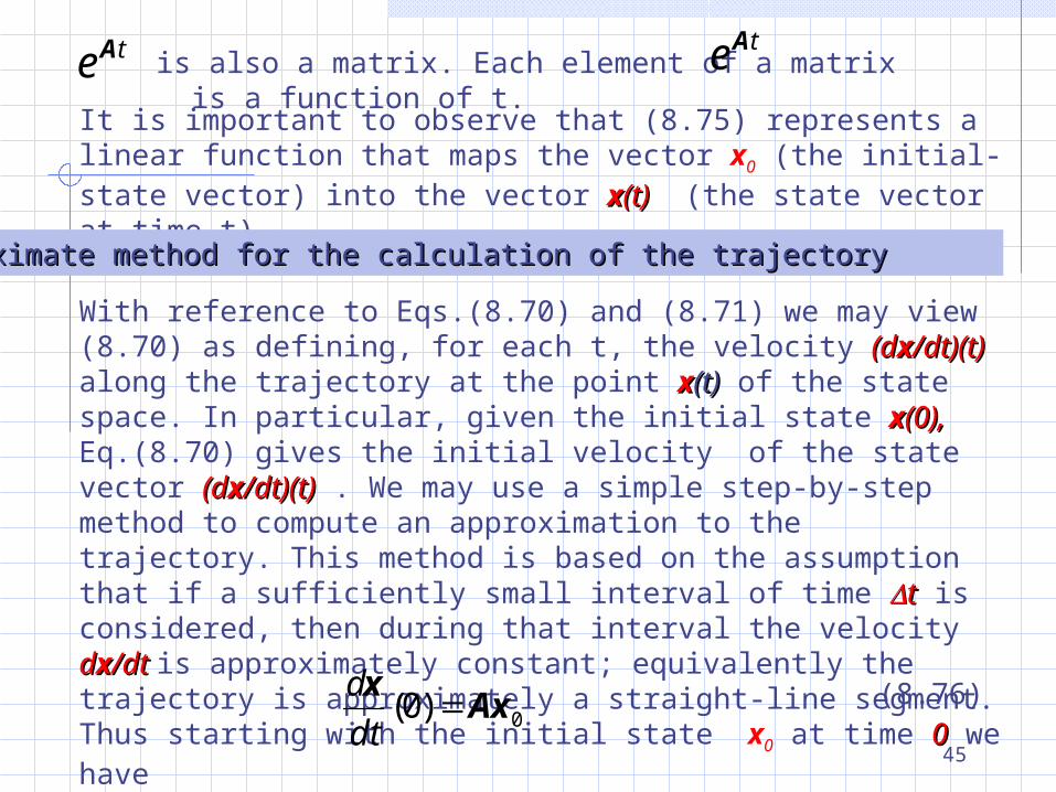
teA is also a matrix. Each element of a matrix is a function of t.

teA

It is important to observe that (8.75) represents a linear function that maps the vector x0 (the initial-state vector) into the vector xx(t)(t) (the state vector at time t).

Approximate method for the calculation of the trajectoryApproximate method for the calculation of the trajectory

With reference to Eqs.(8.70) and (8.71) we may view (8.70) as defining, for each t, the velocity (d(dxx/dt)(t)/dt)(t) along the trajectory at the point xx(t)(t) of the state space. In particular, given the initial state xx(0),(0), Eq.(8.70) gives the initial velocity of the state vector (d(dxx/dt)(t)/dt)(t) . We may use a simple step-by-step method to compute an approximation to the trajectory. This method is based on the assumption that if a sufficiently small interval of time tt is considered, then during that interval the velocity ddxx/dt /dt is approximately constant; equivalently the trajectory is approximately a straight-line segment. Thus starting with the initial state x0 at time 00 we have

0)0( Axx

dt

d (8.76)

46

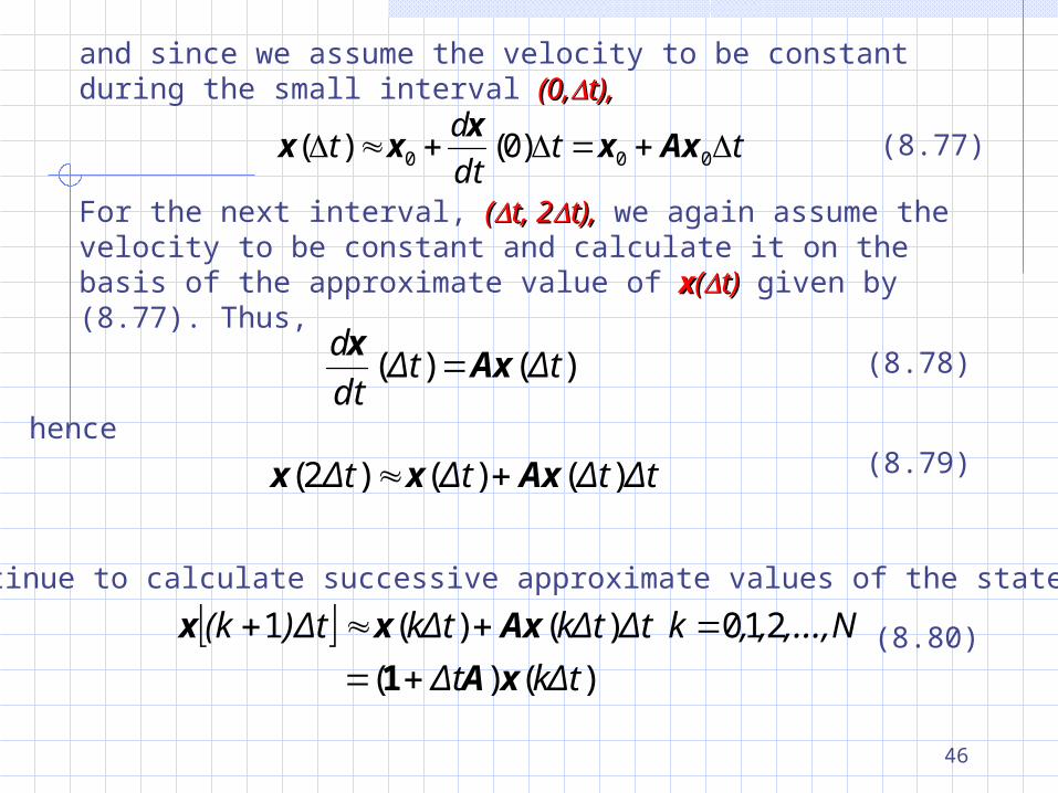
and since we assume the velocity to be constant during the small interval (0,(0,t),t),

ttdt

dt 000 )0()( Axx

xxx (8.77)

For the next interval, ((t, 2t, 2t),t), we again assume the velocity to be constant and calculate it on the basis of the approximate value of xx((t)t) given by (8.77). Thus,

)()( tΔtΔdt

dAx

x (8.78)

tΔtΔtΔtΔ )()()2( Axxx hence

(8.79)

We continue to calculate successive approximate values of the state

)()(

210 )()(1

tΔktΔ

,...,N,,ktΔtΔktΔktΔ)(k

xA

Axxx

1(8.80)

47

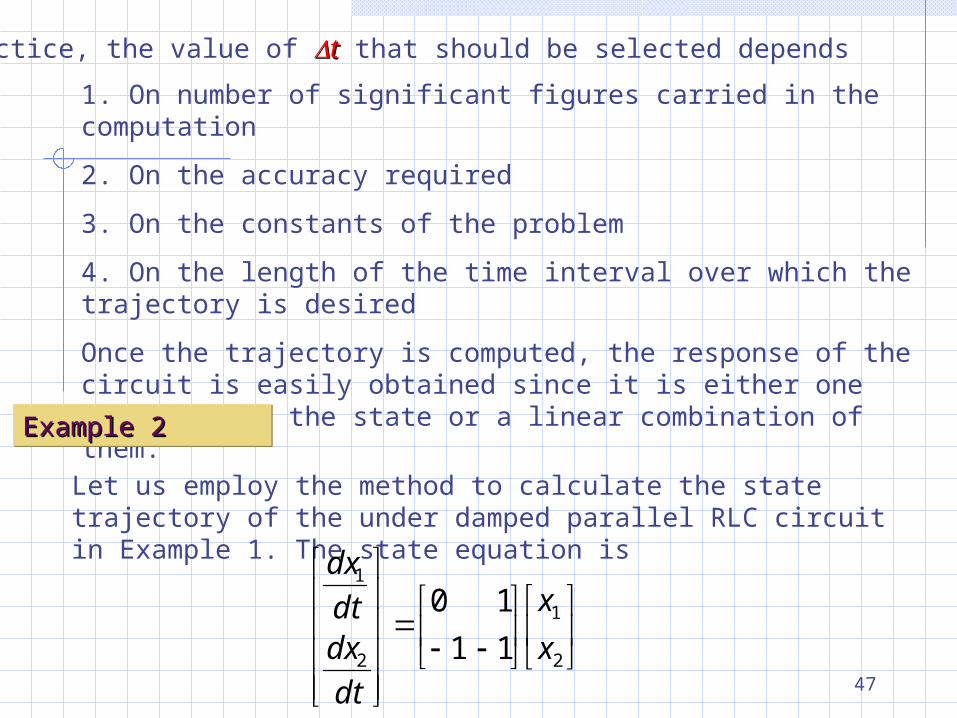
In practice, the value of tt that should be selected depends

1. On number of significant figures carried in the computation

2. On the accuracy required

3. On the constants of the problem

4. On the length of the time interval over which the trajectory is desired

Once the trajectory is computed, the response of the circuit is easily obtained since it is either one component of the state or a linear combination of them.

Example 2Example 2Example 2Example 2

Let us employ the method to calculate the state trajectory of the under damped parallel RLC circuit in Example 1. The state equation is

2

1

2

1

1 1

1 0

x

x

dt

dxdt

dx

48

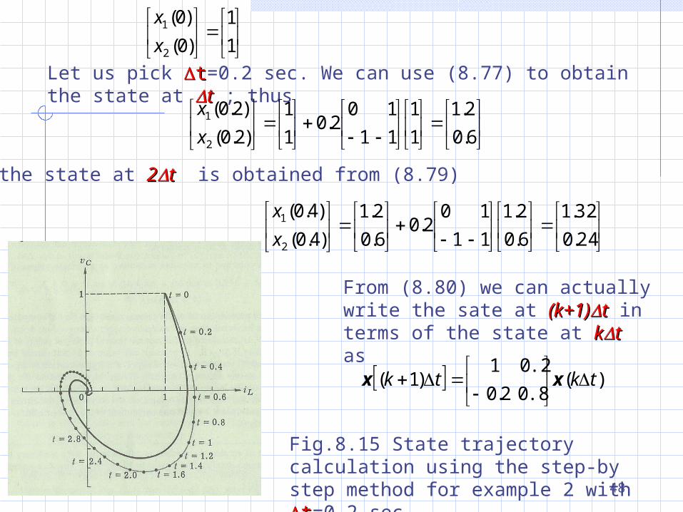
1

1

)0(

)0(

2

1

x

x

Let us pick tt=0.2 sec. We can use (8.77) to obtain the state at tt ; thus

6.0

2.1

1

1

1 1

1 02.0

1

1

)2.0(

)2.0(

2

1

x

x

Next the state at 22tt is obtained from (8.79)

24.0

32.1

6.0

2.1

1 1

1 02.0

6.0

2.1

)4.0(

)4.0(

2

1

x

x

From (8.80) we can actually write the sate at (k+1)(k+1)tt in terms of the state at kktt as

)(.80 2.0

.20 1 )1( tktk

xx

Fig.8.15 State trajectory calculation using the step-by step method for example 2 with tt=0.2 sec.

49

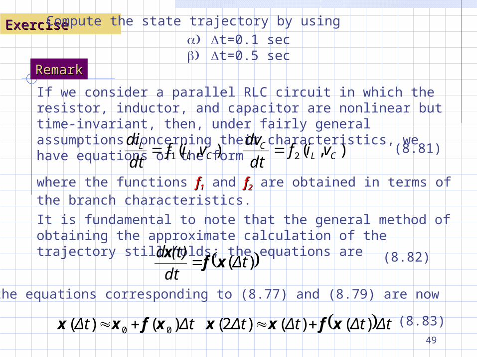
ExerciseExercise Compute the state trajectory by using t=0.1 secb t=0.5 sec

RemarkRemark

If we consider a parallel RLC circuit in which the resistor, inductor, and capacitor are nonlinear but time-invariant, then, under fairly general assumptions concerning their characteristics, we have equations of the form

),( ),( 21 CLC

CLL vif

dt

dvvif

dt

di (8.81)

where the functions ff11 and ff22 are obtained in terms of the branch characteristics.

It is fundamental to note that the general method of obtaining the approximate calculation of the trajectory still holds; the equations are )( tΔ

dt

(t)dx

xf (8.82)

tΔtΔtΔtΔtΔtΔ )()()2( )()( 00 xfxxxfxx

And the equations corresponding to (8.77) and (8.79) are now

(8.83)

50

State Equations and Complete ResponseState Equations and Complete Response

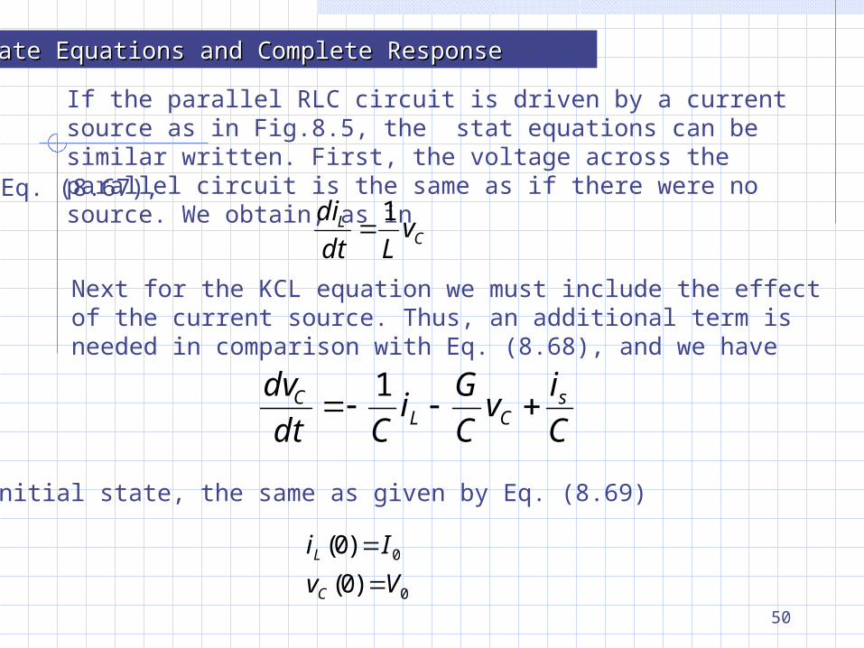
If the parallel RLC circuit is driven by a current source as in Fig.8.5, the stat equations can be similar written. First, the voltage across the parallel circuit is the same as if there were no source. We obtain, as in Eq. (8.67),

CL v

Ldt

di 1

Next for the KCL equation we must include the effect of the current source. Thus, an additional term is needed in comparison with Eq. (8.68), and we have

C

iv

C

Gi

Cdt

dv sCL

C 1

The initial state, the same as given by Eq. (8.69)

0

0

)0(

)0(

Vv

Ii

C

L

51

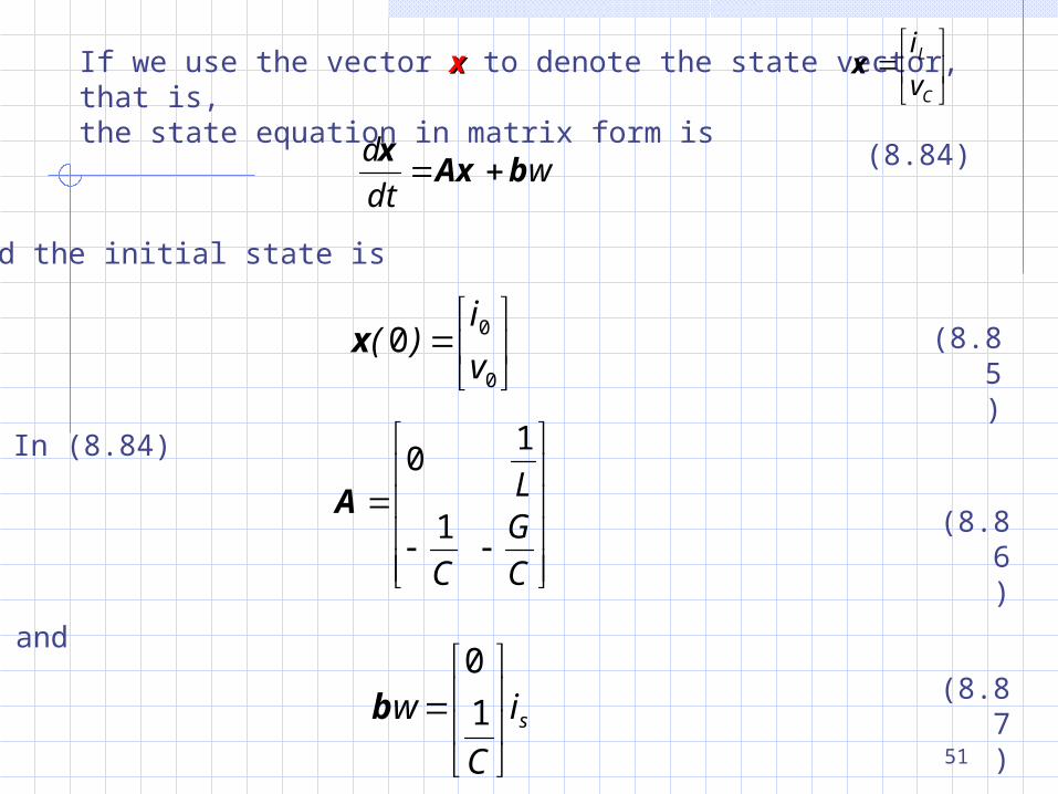
If we use the vector xx to denote the state vector, that is, the state equation in matrix form is

C

L

v

ix

wdt

dbAx

x (8.84)

and the initial state is

0

00v

i)(x (8.85

)

In (8.84)

C

G

C

L

1

1 0

A(8.86

)

and

si

C

w

1

0b

(8.87)

52

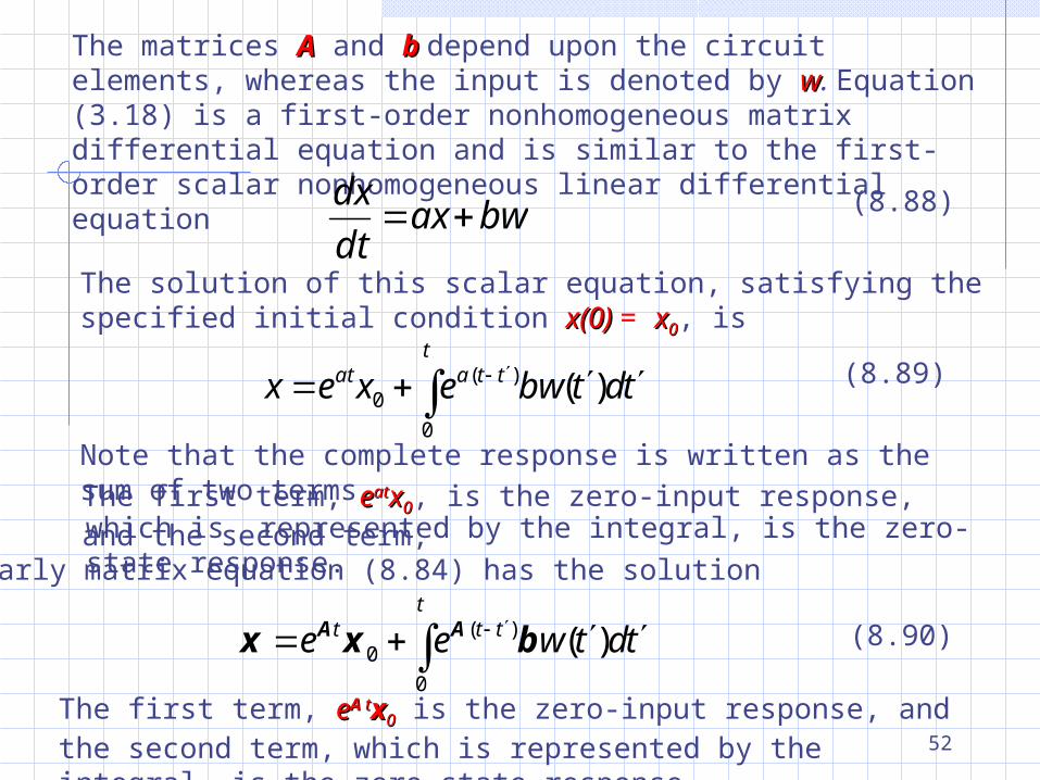
The matrices AA and b b depend upon the circuit elements, whereas the input is denoted by ww. Equation (3.18) is a first-order nonhomogeneous matrix differential equation and is similar to the first-order scalar nonhomogeneous linear differential equation

bwaxdt

dx (8.88)

The solution of this scalar equation, satisfying the specified initial condition x(0)x(0) = xx00, is

t

ttaat tdtbwexex0

)(0 )( (8.89)

Note that the complete response is written as the sum of two terms. The first term, eeatatxx00, is the zero-input response, and the second term, which is represented by the integral, is the zero-state response. Similarly matrix equation (8.84) has the solution

t

ttt tdtwee0

)(0 )(bxx AA (8.90)

The first term, eeA A ttxx00 is the zero-input response, and the second term, which is represented by the integral, is the zero-state response.