1

LEARNINGLEARNING

Adopted from slides and notes by Tim Finin, Marie desJardins andChuck Dyer

2

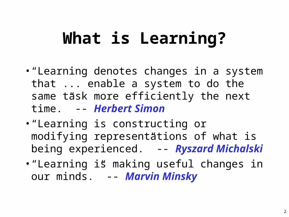
What is Learning?

• “Learning denotes changes in a system that ... enable a system to do the same task more efficiently the next time.” -- Herbert Simon

• “Learning is constructing or modifying representations of what is being experienced.” -- Ryszard Michalski

• “Learning is making useful changes in our minds.” -- Marvin Minsky

3

Why Learn?• Understand and improve efficiency of human learning

– Use to improve methods for teaching and tutoring people (e.g., better computer-aided instruction.)

• Discover new things or structures that are unknown to humans– Example: Data mining, Knowledge Discovery in Databases

• Fill in skeletal or incomplete specifications about a domain– Large, complex AI systems cannot be completely derived by hand and

require dynamic updating to incorporate new information.

– Learning new characteristics expands the domain or expertise and lessens the "brittleness" of the system

• Build software agents that can adapt to their users, to other software agents, and to the changing environment.

4

A General Model of Learning Agents

5

Major Paradigms of Machine Learning

• Rote Learning -- One-to-one mapping from inputs to stored representation. "Learning by memorization.” Association-based storage and retrieval.

• Clustering• Analogue -- Determine correspondence between two different

representations • Induction -- Use specific examples to reach general conclusions• Discovery -- Unsupervised, specific goal not given • Genetic Algorithms• Neural Networks• Reinforcement -- Feedback (positive or negative reward) given at

end of a sequence of steps. – Assign reward to steps by solving the credit assignment problem--which

steps should receive credit or blame for a final result?

6

The Inductive Learning Problem• Induce rules that extrapolate from a given set of examples

to make “accurate” predictions about future examples.

• Supervised versus Unsupervised learning– Learn an unknown function f(X) = Y, where X is an input example

and Y is the desired output.

– Supervised learning implies we are given a training set of (X, Y) pairs by a "teacher."

– Unsupervised learning means we are only given the Xs and some (ultimate) feedback function on our performance.

• Concept learning or Classification– Given a set of examples of some concept/class/category, determine

if a given example is an instance of the concept or not.

– If it is an instance, we call it a positive example.

– If it is not, it is called a negative example.

7

Supervised Concept Learning

• Given a training set of positive and negative examples of a concept– Usually each example has a set of features/attributes

• Construct a description that will accurately classify whether future examples are positive or negative.

• That is, learn some good estimate of function f given a training set {(x1, y1), (x2, y2), ..., (xn, yn)} where each yi is either + (positive) or - (negative). – f is a function of the features/attributes

8

Inductive Learning Framework

• Raw input data from sensors are preprocessed to obtain a feature vector, X, that adequately describes all of the relevant features for classifying examples.

• Each x is a list of (attribute, value) pairs. For example, X = [Person:Sue, EyeColor:Brown, Age:Young, Sex:Female]

• The number and names of attributes (aka features) is fixed (positive, finite).

• Each attribute has a fixed, finite number of possible values.

• Each example can be interpreted as a point in an n-dimensional feature space, where n is the number of attributes.

9

Inductive Learning by Nearest-Neighbor Classification

• One simple approach to inductive learning is to save each training example as a point in feature space

• Classify a new example by giving it the same classification (+ or -) as its nearest neighbor in Feature Space.

– A variation involves computing a weighted sum of class of a set of neighbors where the weights correspond to distances

– Another variation uses the center of class

• The problem with this approach is that it doesn't necessarily generalize well if the examples are not well "clustered."

10

Learning Decision Trees• Goal: Build a decision tree for

classifying examples as positive or negative instances of a concept using supervised learning from a training set.

• A decision tree is a tree where– each non-leaf node is associated with an

attribute (feature)– each leaf node is associated with a

classification (+ or -)– each arc is associated with one of the

possible values of the attribute at the node where the arc is directed from.

• Generalization: allow for >2 classes– e.g., {sell, hold, buy}

Color

ShapeSize +

+- Size

+-

+big

big small

small

roundsquare

redgreen blue

11

Preference Bias: Ockham's Razor• Aka Occam’s Razor, Law of Economy, or Law of Parsimony

• Principle stated by William of Ockham (1285-1347/49), a scholastic, that – “non sunt multiplicanda entia praeter necessitatem” – or, entities are not to be multiplied beyond necessity.

• The simplest explanation that is consistent with all observations is the best.

• Therefor, the smallest decision tree that correctly classifies all of the training examples is best.

• Finding the provably smallest decision tree is NP-Hard, so instead of constructing the absolute smallest tree consistent with the training examples, construct one that is pretty small.

12

Inductive Learning and Bias

• Suppose that we want to learn a function f(x) = y and we are given some sample (x,y) pairs, as in figure (a).

• There are several hypotheses we could make about this function, e.g.: (b), (c) and (d).

• A preference for one over the others reveals the bias of our learning technique, e.g.:– prefer piece-wise functions– prefer a smooth function– prefer a simple function and treat outliers as noise

13

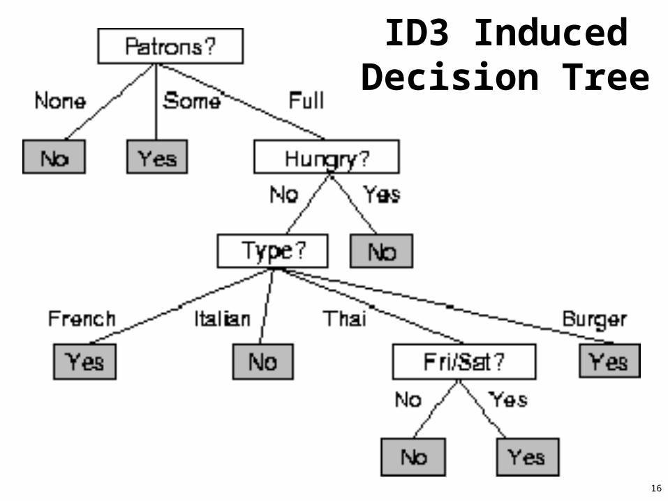
R&Ns Restaurant Domain

• Develop a decision tree to model the decision a patron makes when deciding whether or not to wait for a table at a restaurant.

• Two classes: wait, leave• Ten attributes: alternative restaurant available?, bar in

restaurant?, is it Friday?, are we hungry?, how full is the restaurant?, how expensive?, is it raining?,do we have a reservation?, what type of restaurant is it?, what's the purported waiting time?

• Training set of 12 examples• ~ 7000 possible cases

14

A Training Set

15

A decision Treefrom Introspection

16

ID3 Induced Decision Tree

17

ID3• A greedy algorithm for Decision Tree Construction

developed by Ross Quinlan, 1987 • Consider a smaller tree a better tree• Top-down construction of the decision tree by recursively

selecting the "best attribute" to use at the current node in the tree, based on the examples belonging to this node. – Once the attribute is selected for the current node,

generate children nodes, one for each possible value of the selected attribute.

– Partition the examples of this node using the possible values of this attribute, and assign these subsets of the examples to the appropriate child node.

– Repeat for each child node until all examples associated with a node are either all positive or all negative.

18

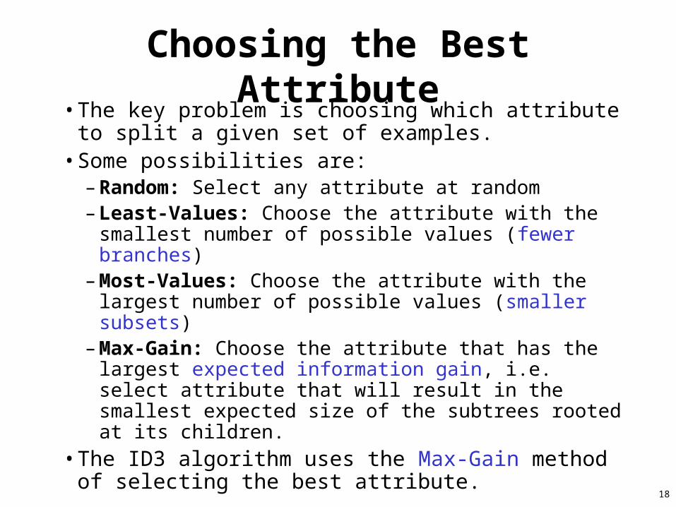
Choosing the Best Attribute• The key problem is choosing which attribute to split a

given set of examples. • Some possibilities are:

– Random: Select any attribute at random – Least-Values: Choose the attribute with the smallest

number of possible values (fewer branches)– Most-Values: Choose the attribute with the largest

number of possible values (smaller subsets)– Max-Gain: Choose the attribute that has the largest

expected information gain, i.e. select attribute that will result in the smallest expected size of the subtrees rooted at its children.

• The ID3 algorithm uses the Max-Gain method of selecting the best attribute.

19

Splitting Examples by Testing Attributes

20

ID3 Induced Decision Tree

21

Another example: tennis anyone?

22

Choosing the first split

23

Resulting Decision Tree

24

Information Theory Background

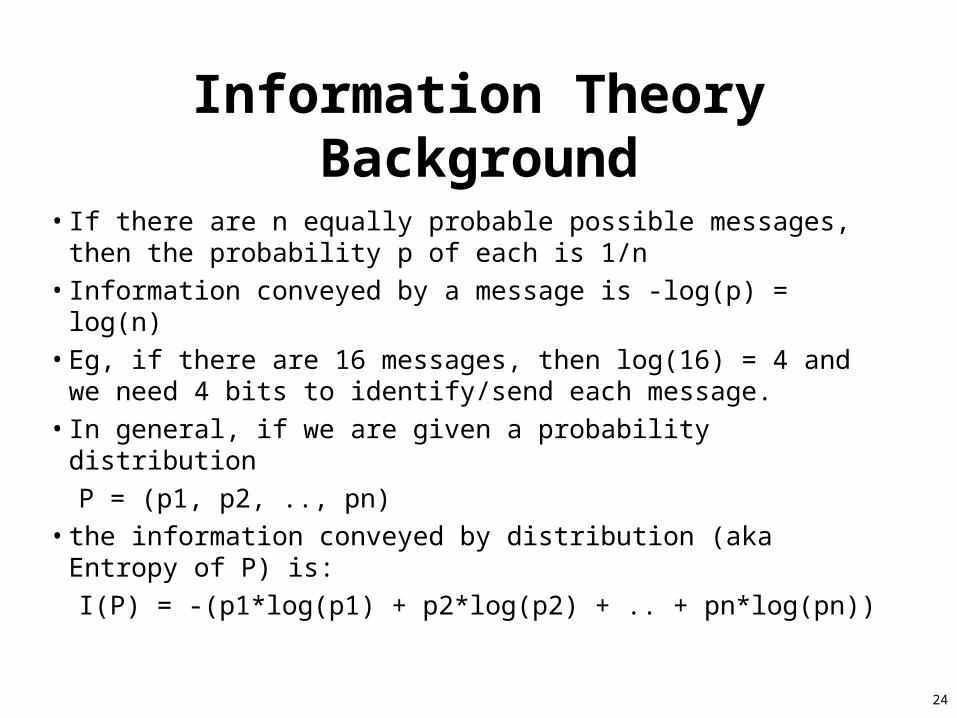
• If there are n equally probable possible messages, then the probability p of each is 1/n

• Information conveyed by a message is -log(p) = log(n)

• Eg, if there are 16 messages, then log(16) = 4 and we need 4 bits to identify/send each message.

• In general, if we are given a probability distribution

P = (p1, p2, .., pn)

• the information conveyed by distribution (aka Entropy of P) is:

I(P) = -(p1*log(p1) + p2*log(p2) + .. + pn*log(pn))

25

• The entropy is the average number of bits/message needed to represent a stream of messages.

• Examples:

– if P is (0.5, 0.5) then I(P) is 1

– if P is (0.67, 0.33) then I(P) is 0.92, – if P is (1, 0) then I(P) is 0.

• The more uniform is the probability distribution, the greater is its information gain/entropy.

26

Example: Huffman code• In 1952 MIT student David Huffman devised, in the course of

doing a homework assignment, an elegant coding scheme which is optimal in the case where all symbols probabilities are integral powers of 1/2.

• A Huffman code can be built in the following manner:

– Rank all symbols in order of probability of occurrence.

– Successively combine the two symbols of the lowest probability to form a new composite symbol; eventually we will build a binary tree where each node is the probability of all nodes beneath it.

– Trace a path to each leaf, noticing the direction at each node.

27

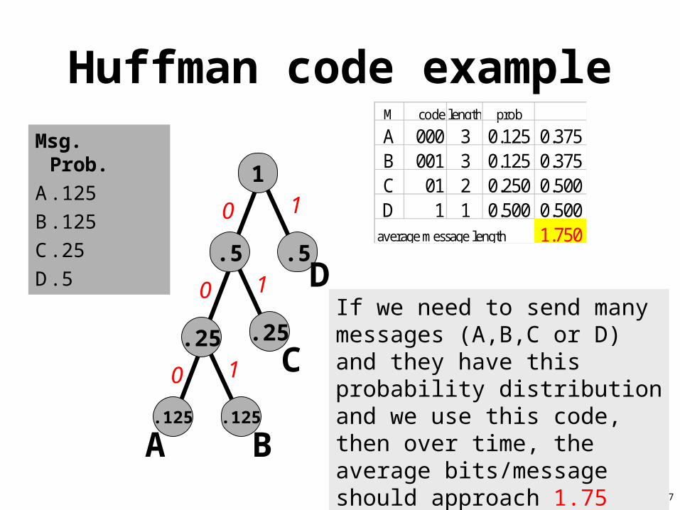
Huffman code example

Msg. Prob.

A .125

B .125

C .25

D .5 .5.5

1

.125.125

.25

A

C

B

D

.25

0 1

0

0 1

1

M code length prob

A 000 3 0.125 0.375B 001 3 0.125 0.375C 01 2 0.250 0.500D 1 1 0.500 0.500

average message length 1.750

If we need to send many messages (A,B,C or D) and they have this probability distribution and we use this code, then over time, the average bits/message should approach 1.75 (= 0.125*3+0.125*3+0.25*2*0.5*1)

28

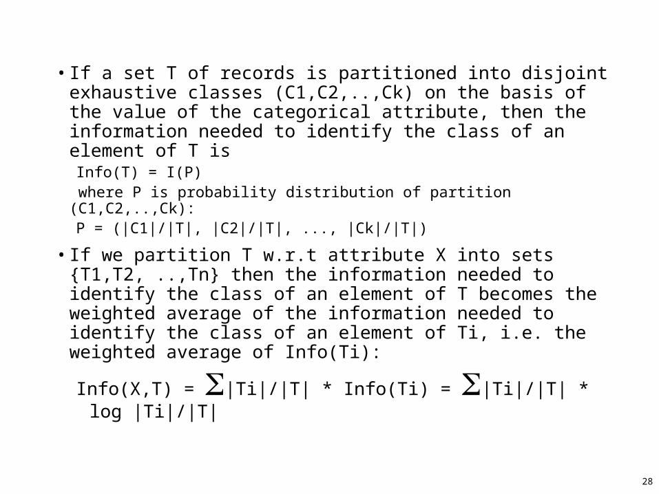
• If a set T of records is partitioned into disjoint exhaustive classes (C1,C2,..,Ck) on the basis of the value of the categorical attribute, then the information needed to identify the class of an element of T is Info(T) = I(P)

where P is probability distribution of partition (C1,C2,..,Ck): P = (|C1|/|T|, |C2|/|T|, ..., |Ck|/|T|)

• If we partition T w.r.t attribute X into sets {T1,T2, ..,Tn} then the information needed to identify the class of an element of T becomes the weighted average of the information needed to identify the class of an element of Ti, i.e. the weighted average of Info(Ti):

Info(X,T) = |Ti|/|T| * Info(Ti) = |Ti|/|T| * log |Ti|/|T|

29

Gain• Consider the quantity Gain(X,T) defined as Gain(X,T) = Info(T) - Info(X,T)• This represents the difference between

– information needed to identify an element of T and – information needed to identify an element of T after the value of

attribute X has been obtained,

that is, this is the gain in information due to attribute X.• We can use this to rank attributes and to build decision trees

where at each node is located the attribute with greatest gain among the attributes not yet considered in the path from the root.

• The intent of this ordering are twofold:– To create small decision trees so that records can be identified after

only a few questions.– To match a hoped for minimality of the process represented by the

records being considered (Occam's Razor).

30

The ID3 algorithm is used to build a decision tree, given a set of non-categorical attributes C1, C2, .., Cn, the categorical attribute C, and a training set T of records.

function ID3 (R: a set of non-categorical attributes,

C: the categorical attribute,

S: a training set) returns a decision tree;

begin

If S is empty, return a single node with value Failure;

If every example in S has the same value for categorical

attribute, return single node with that value;

If R is empty, then return a single node with most

frequent of the values of the categorical attribute found in

examples S; [note: there will be errors, i.e., improperly

classified records];

Let D be attribute with largest Gain(D,S) among R’s attributes;

Let {dj| j=1,2, .., m} be the values of attribute D;

Let {Sj| j=1,2, .., m} be the subsets of S consisting

respectively of records with value dj for attribute D;

Return a tree with root labeled D and arcs labeled

d1, d2, .., dm going respectively to the trees

ID3(R-{D},C,S1), ID3(R-{D},C,S2) ,.., ID3(R-{D},C,Sm);

end ID3;

31

How well does it work?Many case studies have shown that decision trees are at least as accurate as human experts. – A study for diagnosing breast cancer had humans

correctly classifying the examples 65% of the time, and the decision tree classified 72% correct.

– British Petroleum designed a decision tree for gas-oil separation for offshore oil platforms that replaced an earlier rule-based expert system.

– Cessna designed an airplane flight controller using 90,000 examples and 20 attributes per example.

32

Extensions of the Decision Tree Learning Algorithm

• Using gain ratios

• Real-valued data

• Noisy data and Overfitting

• Generation of rules

• Setting Parameters

• Cross-Validation for Experimental Validation of Performance

• C4.5 (and C5.0) is an extension of ID3 that accounts for unavailable values, continuous attribute value ranges, pruning of decision trees, rule derivation, and so on.

• Incremental learning

33

Using Gain Ratios• The notion of Gain introduced earlier favors attributes that have

a large number of values. – If we have an attribute D that has a distinct value for each

record, then Info(D,T) is 0, thus Gain(D,T) is maximal.

• To compensate for this Quinlan suggests using the following ratio instead of Gain:

GainRatio(D,T) = Gain(D,T) / SplitInfo(D,T)

• SplitInfo(D,T) is the information due to the split of T on the basis of value of categorical attribute D.

SplitInfo(D,T) = I(|T1|/|T|, |T2|/|T|, .., |Tm|/|T|)

where {T1, T2, .. Tm} is the partition of T induced by value of D.

34

Real-valued data

• Select a set of thresholds defining intervals; • each interval becomes a discrete value of the attribute• We can use some simple heuristics

– always divide into quartiles

• We can use domain knowledge– divide age into infant (0-2), toddler (3 - 5), and school aged (5-

8)

• or treat this as another learning problem – try a range of ways to discretize the continuous variable and see

which yield “better results” w.r.t. some metric.

35

Noisy data and Overfitting• Many kinds of "noise" that could occur in the examples:

– Two examples have same attribute/value pairs, but different classifications

– Some values of attributes are incorrect because of errors in the data acquisition process or the preprocessing phase

– The classification is wrong (e.g., + instead of -) because of some error

• Some attributes are irrelevant to the decision-making process,– e.g., color of a die is irrelevant to its outcome.

– Irrelevant attributes can result in overfitting the training data.

• Overfitting: – learning result fits data (training examples) well but does not hold for

unseen data (poor generalization)

– Often need to compromise fitness to data and generalization power

– Overfitting is a problem common to all methods that learn from data

36

• Fix overfitting/overlearning problem– By cross validation (see later)

– By pruning lower nodes in the decision tree.

For example, if Gain of the best attribute at a node is below a threshold, stop and make this node a leaf rather than generating children nodes.

(b and (c): better fit for data, poor generalization

(d): not fit for the outlier (possibly due to noise), but better generalization

37

Pruning Decision Trees• Pruning of the decision tree is done by replacing a whole

subtree by a leaf node. • The replacement takes place if a decision rule establishes

that the expected error rate in the subtree is greater than in the single leaf. E.g.,– Training: eg, one training red success and one training blue Failures– Test: three red failures and one blue success– Consider replacing this subtree by a single Failure node.

• After replacement we will have only two errors instead of five failures.

Color

1 success0 failure

0 success1 failure

red blue

Color

1 success3 failure

1 success1 failure

red blue 2 success4 failure

FAILURE

38

Incremental Learning

• Incremental learning– Change can be made with each training example

– Non-incremental learning is also called batch learning

– Good for • adaptive system (learning while experiencing)

• when environment undergoes changes – Often with

• Higher computational cost

• Lower quality of learning results

– ITI (by U. Mass): incremental DT learning package

39

Evaluation Methodology• Standard methodology: cross validation

1. Collect a large set of examples (all with correct classifications!).2. Randomly divide collection into two disjoint sets: training and test.3. Apply learning algorithm to training set giving hypothesis H4. Measure performance of H w.r.t. test set

• Important: keep the training and test sets disjoint!• Learning is not to minimize training error (wrt data) but the

error for test/cross-validation: a way to fix overfitting• To study the efficiency and robustness of an algorithm, repeat

steps 2-4 for different training sets and sizes of training sets.• If you improve your algorithm, start again with step 1 to avoid

evolving the algorithm to work well on just this collection.

40

Restaurant ExampleLearning Curve

41

Decision Trees to Rules

• It is easy to derive a rule set from a decision tree: write a rule for each path in the decision tree from the root to a leaf.

• In that rule the left-hand side is easily built from the label of the nodes and the labels of the arcs.

• The resulting rules set can be simplified:– Let LHS be the left hand side of a rule.

– Let LHS' be obtained from LHS by eliminating some conditions.

– We can certainly replace LHS by LHS' in this rule if the subsets of the training set that satisfy respectively LHS and LHS' are equal.

– A rule may be eliminated by using metaconditions such as "if no other rule applies".

42

C4.5• C4.5 is an extension of ID3 that accounts for unavailable

values, continuous attribute value ranges, pruning of decision trees, rule derivation, and so on.

C4.5: Programs for Machine LearningJ. Ross Quinlan, The Morgan Kaufmann Series

in Machine Learning, Pat Langley,

Series Editor. 1993. 302 pages. paperback book & 3.5" Sun disk. $77.95. ISBN 1-55860-240-2

43

Summary of DT Learning• Inducing decision trees is one of the most widely used

learning methods in practice

• Can out-perform human experts in many problems

• Strengths include– Fast– simple to implement– can convert result to a set of easily interpretable rules– empirically valid in many commercial products– handles noisy data

• Weaknesses include:– "Univariate" splits/partitioning using only one attribute at a time so

limits types of possible trees

– large decision trees may be hard to understand

– requires fixed-length feature vectors