1

Knowledge Knowledge Representation and Representation and

ReasoningReasoningChapter 10.1-10.2, 10.6

CS 63CS 63

Adapted from slides byTim Finin andMarie desJardins.

Some material adopted from notes by Andreas Geyer-Schulz,

and Chuck Dyer.

2

Abduction• Abduction is a reasoning process that tries to form plausible

explanations for abnormal observations– Abduction is distinctly different from deduction and induction– Abduction is inherently uncertain

• Uncertainty is an important issue in abductive reasoning• Some major formalisms for representing and reasoning about

uncertainty– Mycin’s certainty factors (an early representative)– Probability theory (esp. Bayesian belief networks)– Dempster-Shafer theory– Fuzzy logic– Truth maintenance systems– Nonmonotonic reasoning

3

Abduction• Definition (Encyclopedia Britannica): reasoning that derives

an explanatory hypothesis from a given set of facts– The inference result is a hypothesis that, if true, could

explain the occurrence of the given facts• Examples

– Dendral, an expert system to construct 3D structure of chemical compounds • Fact: mass spectrometer data of the compound and its

chemical formula• KB: chemistry, esp. strength of different types of bounds• Reasoning: form a hypothetical 3D structure that satisfies the

chemical formula, and that would most likely produce the given mass spectrum

4

– Medical diagnosis• Facts: symptoms, lab test results, and other observed findings

(called manifestations)

• KB: causal associations between diseases and manifestations

• Reasoning: one or more diseases whose presence would causally explain the occurrence of the given manifestations

– Many other reasoning processes (e.g., word sense disambiguation in natural language process, image understanding, criminal investigation) can also been seen as abductive reasoning

Abduction examples (cont.)

5

Comparing abduction, deduction, and induction

Deduction: major premise: All balls in the box are black minor premise: These balls are from the box conclusion: These balls are black

Abduction: rule: All balls in the box are black observation: These balls are black explanation: These balls are from the box

Induction: case: These balls are from the box observation: These balls are black hypothesized rule: All ball in the box are black

A => B A ---------B

A => B B-------------Possibly A

Whenever A then B-------------Possibly A => B

Deduction reasons from causes to effectsAbduction reasons from effects to causesInduction reasons from specific cases to general rules

6

Characteristics of abductive reasoning

• “Conclusions” are hypotheses, not theorems (may be false even if rules and facts are true)

– E.g., misdiagnosis in medicine

• There may be multiple plausible hypotheses– Given rules A => B and C => B, and fact B, both A and C

are plausible hypotheses – Abduction is inherently uncertain– Hypotheses can be ranked by their plausibility (if it can be

determined)

7

Characteristics of abductive reasoning (cont.)

• Reasoning is often a hypothesize-and-test cycle – Hypothesize: Postulate possible hypotheses, any of which would

explain the given facts (or at least most of the important facts)– Test: Test the plausibility of all or some of these hypotheses– One way to test a hypothesis H is to ask whether something that is

currently unknown–but can be predicted from H–is actually true• If we also know A => D and C => E, then ask if D and E are

true• If D is true and E is false, then hypothesis A becomes more

plausible (support for A is increased; support for C is decreased)

8

Characteristics of abductive reasoning (cont.)

• Reasoning is non-monotonic – That is, the plausibility of hypotheses can

increase/decrease as new facts are collected – In contrast, deductive inference is monotonic: it never

change a sentence’s truth value, once known– In abductive (and inductive) reasoning, some

hypotheses may be discarded, and new ones formed, when new observations are made

9

Sources of uncertainty

• Uncertain inputs– Missing data– Noisy data

• Uncertain knowledge– Multiple causes lead to multiple effects– Incomplete enumeration of conditions or effects– Incomplete knowledge of causality in the domain– Probabilistic/stochastic effects

• Uncertain outputs– Abduction and induction are inherently uncertain– Default reasoning, even in deductive fashion, is uncertain– Incomplete deductive inference may be uncertain

Probabilistic reasoning only gives probabilistic results (summarizes uncertainty from various sources)

10

Decision making with uncertainty

• Rational behavior:

– For each possible action, identify the possible outcomes

– Compute the probability of each outcome

– Compute the utility of each outcome

– Compute the probability-weighted (expected) utility over possible outcomes for each action

– Select the action with the highest expected utility (principle of Maximum Expected Utility)

11

Bayesian reasoning

• Probability theory

• Bayesian inference– Use probability theory and information about independence

– Reason diagnostically (from evidence (effects) to conclusions (causes)) or causally (from causes to effects)

• Bayesian networks– Compact representation of probability distribution over a set of

propositional random variables

– Take advantage of independence relationships

12

Other uncertainty representations• Default reasoning

– Nonmonotonic logic: Allow the retraction of default beliefs if they prove to be false

• Rule-based methods– Certainty factors (Mycin): propagate simple models of belief

through causal or diagnostic rules

• Evidential reasoning– Dempster-Shafer theory: Bel(P) is a measure of the evidence for P;

Bel(P) is a measure of the evidence against P; together they define a belief interval (lower and upper bounds on confidence)

• Fuzzy reasoning– Fuzzy sets: How well does an object satisfy a vague property?– Fuzzy logic: “How true” is a logical statement?

13

Uncertainty tradeoffs• Bayesian networks: Nice theoretical properties combined

with efficient reasoning make BNs very popular; limited expressiveness, knowledge engineering challenges may limit uses

• Nonmonotonic logic: Represent commonsense reasoning, but can be computationally very expensive

• Certainty factors: Not semantically well founded• Dempster-Shafer theory: Has nice formal properties, but

can be computationally expensive, and intervals tend to grow towards [0,1] (not a very useful conclusion)

• Fuzzy reasoning: Semantics are unclear (fuzzy!), but has proved very useful for commercial applications

14

Bayesian ReasoningBayesian Reasoning

Chapter 13

CS 63CS 63

Adapted from slides byTim Finin andMarie desJardins.

15

Outline

• Probability theory

• Bayesian inference– From the joint distribution

– Using independence/factoring

– From sources of evidence

16

Sources of uncertainty

• Uncertain inputs– Missing data– Noisy data

• Uncertain knowledge– Multiple causes lead to multiple effects– Incomplete enumeration of conditions or effects– Incomplete knowledge of causality in the domain– Probabilistic/stochastic effects

• Uncertain outputs– Abduction and induction are inherently uncertain– Default reasoning, even in deductive fashion, is uncertain– Incomplete deductive inference may be uncertain

Probabilistic reasoning only gives probabilistic results (summarizes uncertainty from various sources)

17

Decision making with uncertainty

• Rational behavior:

– For each possible action, identify the possible outcomes

– Compute the probability of each outcome

– Compute the utility of each outcome

– Compute the probability-weighted (expected) utility over possible outcomes for each action

– Select the action with the highest expected utility (principle of Maximum Expected Utility)

18

Why probabilities anyway?• Kolmogorov showed that three simple axioms lead to the

rules of probability theory– De Finetti, Cox, and Carnap have also provided compelling

arguments for these axioms

1. All probabilities are between 0 and 1:• 0 ≤ P(a) ≤ 1

2. Valid propositions (tautologies) have probability 1, and unsatisfiable propositions have probability 0:

• P(true) = 1 ; P(false) = 0

3. The probability of a disjunction is given by:• P(a b) = P(a) + P(b) – P(a b)

aba b

19

Probability theory

• Random variables– Domain

• Atomic event: complete specification of state

• Prior probability: degree of belief without any other evidence

• Joint probability: matrix of combined probabilities of a set of variables

• Alarm, Burglary, Earthquake– Boolean (like these), discrete,

continuous

• (Alarm=True Burglary=True Earthquake=False) or equivalently(alarm burglary ¬earthquake)

• P(Burglary) = 0.1

• P(Alarm, Burglary) =

alarm ¬alarm

burglary 0.09 0.01

¬burglary 0.1 0.8

20

Probability theory (cont.)

• Conditional probability: probability of effect given causes

• Computing conditional probs:– P(a | b) = P(a b) / P(b)

– P(b): normalizing constant

• Product rule:– P(a b) = P(a | b) P(b)

• Marginalizing:– P(B) = ΣaP(B, a)

– P(B) = ΣaP(B | a) P(a) (conditioning)

• P(burglary | alarm) = 0.47P(alarm | burglary) = 0.9

• P(burglary | alarm) = P(burglary alarm) / P(alarm) = 0.09 / 0.19 = 0.47

• P(burglary alarm) = P(burglary | alarm) P(alarm) = 0.47 * 0.19 = 0.09

• P(alarm) = P(alarm burglary) + P(alarm ¬burglary) = 0.09 + 0.1 = 0.19

21

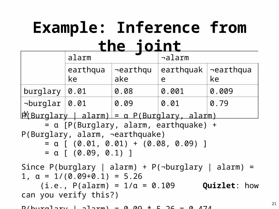
Example: Inference from the jointalarm ¬alarm

earthquake ¬earthquake earthquake ¬earthquake

burglary 0.01 0.08 0.001 0.009

¬burglary 0.01 0.09 0.01 0.79

P(Burglary | alarm) = α P(Burglary, alarm) = α [P(Burglary, alarm, earthquake) + P(Burglary, alarm, ¬earthquake) = α [ (0.01, 0.01) + (0.08, 0.09) ] = α [ (0.09, 0.1) ]

Since P(burglary | alarm) + P(¬burglary | alarm) = 1, α = 1/(0.09+0.1) = 5.26 (i.e., P(alarm) = 1/α = 0.109 Quizlet: how can you verify this?)

P(burglary | alarm) = 0.09 * 5.26 = 0.474

P(¬burglary | alarm) = 0.1 * 5.26 = 0.526

22

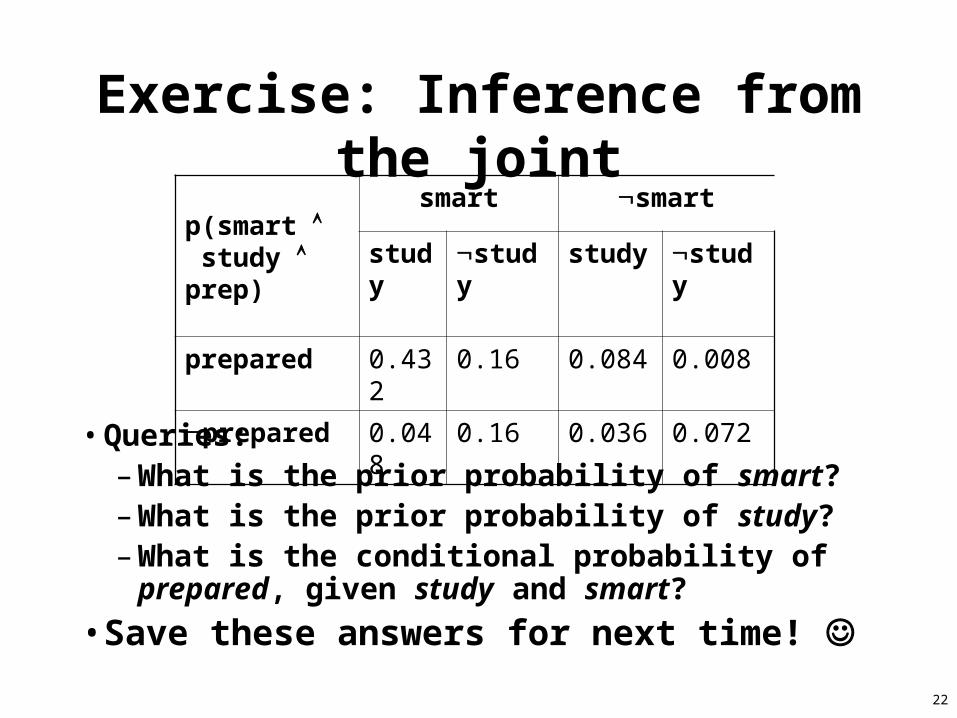
Exercise: Inference from the joint

• Queries:– What is the prior probability of smart?– What is the prior probability of study?– What is the conditional probability of prepared, given

study and smart?

• Save these answers for next time!

p(smart study prep)

smart smart

study study study study

prepared 0.432 0.16 0.084 0.008

prepared 0.048 0.16 0.036 0.072

23

Independence

• When two sets of propositions do not affect each others’ probabilities, we call them independent, and can easily compute their joint and conditional probability:– Independent (A, B) ↔ P(A B) = P(A) P(B), P(A | B) = P(A)

• For example, {moon-phase, light-level} might be independent of {burglary, alarm, earthquake}– Then again, it might not: Burglars might be more likely to

burglarize houses when there’s a new moon (and hence little light)– But if we know the light level, the moon phase doesn’t affect

whether we are burglarized– Once we’re burglarized, light level doesn’t affect whether the alarm

goes off

• We need a more complex notion of independence, and methods for reasoning about these kinds of relationships

24

Exercise: Independence

• Queries:– Is smart independent of study?– Is prepared independent of study?

p(smart study prep)

smart smart

study study study study

prepared 0.432 0.16 0.084 0.008

prepared 0.048 0.16 0.036 0.072

25

Conditional independence

• Absolute independence:– A and B are independent if and only if P(A B) = P(A) P(B);

equivalently, P(A) = P(A | B) and P(B) = P(B | A)

• A and B are conditionally independent given C if and only if

– P(A B | C) = P(A | C) P(B | C)

• This lets us decompose the joint distribution:– P(A B C) = P(A | C) P(B | C) P(C)

• Moon-Phase and Burglary are conditionally independent given Light-Level

• Conditional independence is weaker than absolute independence, but still useful in decomposing the full joint probability distribution

26

Exercise: Conditional independence

• Queries:– Is smart conditionally independent of prepared, given

study?– Is study conditionally independent of prepared, given

smart?

p(smart study prep)

smart smart

study study study study

prepared 0.432 0.16 0.084 0.008

prepared 0.048 0.16 0.036 0.072

27

Bayes’s rule• Bayes’s rule is derived from the product rule:

– P(Y | X) = P(X | Y) P(Y) / P(X)

• Often useful for diagnosis: – If X are (observed) effects and Y are (hidden) causes,

– We may have a model for how causes lead to effects (P(X | Y))

– We may also have prior beliefs (based on experience) about the frequency of occurrence of effects (P(Y))

– Which allows us to reason abductively from effects to causes (P(Y | X)).

28

Bayesian inference

• In the setting of diagnostic/evidential reasoning

– Know prior probability of hypothesis

conditional probability – Want to compute the posterior probability

• Bayes’ theorem (formula 1):

onsanifestatievidence/m

hypotheses

1 mj

i

EEE

H

)(/)|()()|( jijiji EPHEPHPEHP

)( iHP

)|( ij HEP

)|( ij HEP

)|( ji EHP

)( iHP

… …

29

Simple Bayesian diagnostic reasoning

• Knowledge base:– Evidence / manifestations: E1, …, Em

– Hypotheses / disorders: H1, …, Hn

• Ej and Hi are binary; hypotheses are mutually exclusive (non-overlapping) and exhaustive (cover all possible cases)

– Conditional probabilities: P(Ej | Hi), i = 1, …, n; j = 1, …, m

• Cases (evidence for a particular instance): E1, …, Em

• Goal: Find the hypothesis Hi with the highest posterior

– Maxi P(Hi | E1, …, Em)

30

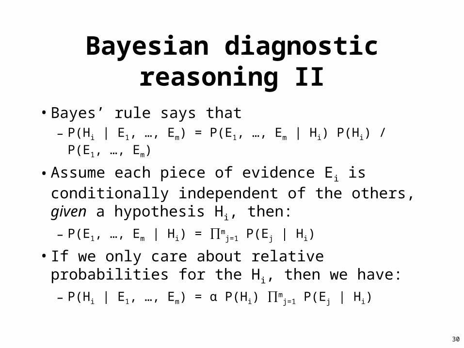
Bayesian diagnostic reasoning II

• Bayes’ rule says that– P(Hi | E1, …, Em) = P(E1, …, Em | Hi) P(Hi) / P(E1, …, Em)

• Assume each piece of evidence Ei is conditionally independent of the others, given a hypothesis Hi, then:

– P(E1, …, Em | Hi) = mj=1 P(Ej | Hi)

• If we only care about relative probabilities for the Hi, then we have:– P(Hi | E1, …, Em) = α P(Hi) m

j=1 P(Ej | Hi)

31

Limitations of simple Bayesian inference

• Cannot easily handle multi-fault situation, nor cases where intermediate (hidden) causes exist:– Disease D causes syndrome S, which causes correlated

manifestations M1 and M2

• Consider a composite hypothesis H1 H2, where H1 and H2 are independent. What is the relative posterior?– P(H1 H2 | E1, …, Em) = α P(E1, …, Em | H1 H2) P(H1 H2)

= α P(E1, …, Em | H1 H2) P(H1) P(H2)= α m

j=1 P(Ej | H1 H2) P(H1) P(H2)

• How do we compute P(Ej | H1 H2) ??

32

Limitations of simple Bayesian inference II

• Assume H1 and H2 are independent, given E1, …, Em?

– P(H1 H2 | E1, …, Em) = P(H1 | E1, …, Em) P(H2 | E1, …, Em)

• This is a very unreasonable assumption– Earthquake and Burglar are independent, but not given Alarm:

• P(burglar | alarm, earthquake) << P(burglar | alarm)

• Another limitation is that simple application of Bayes’s rule doesn’t allow us to handle causal chaining:

– A: this year’s weather; B: cotton production; C: next year’s cotton price

– A influences C indirectly: A→ B → C

– P(C | B, A) = P(C | B)

• Need a richer representation to model interacting hypotheses, conditional independence, and causal chaining

• Next time: conditional independence and Bayesian networks!