Embed Size (px)
Citation preview

1
Introduction to Statistics
Lecture 4
2
Outline
Regression Correlation in more detail Multiple Regression ANCOVA Normality Checks Non-parametrics Sample Size Calculations
3
Linear Regression & Correlation Sometimes we have two quantitative
measurements which are related in some way
e.g. the peak height on a chromatograph and the concentration of analyte in a specimen
They are called the dependent variable (Y) and the independent variable (X)
Y & X may be arbitrary, but if a variable is set by the experimenter rather than simply observed then that variable is X
4
Regression & Correlation
A correlation measures the “degree of association” between two variables (interval (50,100,150…) or ordinal (1,2,3...))
Associations can be positive (an increase in one variable is associated with an increase in the other) or negative (an increase in one variable is associated with a decrease in the other)
5
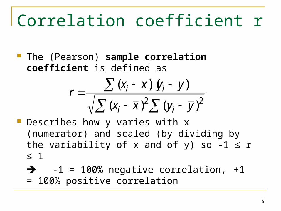
Correlation coefficient r
The (Pearson) sample correlation coefficient is defined as
Describes how y varies with x (numerator) and scaled (by dividing by the variability of x and of y) so -1 ≤ r ≤ 1
-1 = 100% negative correlation, +1 = 100% positive correlation
22 )()(
))((
yyxx
yyxxr
ii
ii
6
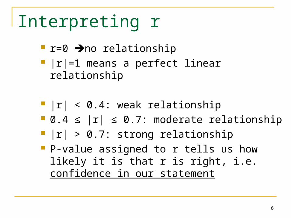
Interpreting r r=0 no relationship |r|=1 means a perfect linear relationship
|r| < 0.4: weak relationship 0.4 ≤ |r| ≤ 0.7: moderate relationship |r| > 0.7: strong relationship P-value assigned to r tells us how likely it is
that r is right, i.e. confidence in our statement
7
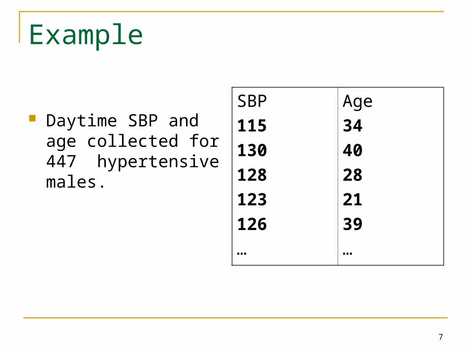
Example
Daytime SBP and age collected for 447 hypertensive males.
SBP
115
130
128
123
126
…
Age
34
40
28
21
39
…

8
Example (contd)
Is there a linear relationship between SBP and Age?
r=0.145 weak positive relationship
9
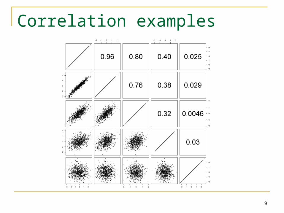
Correlation examples
10
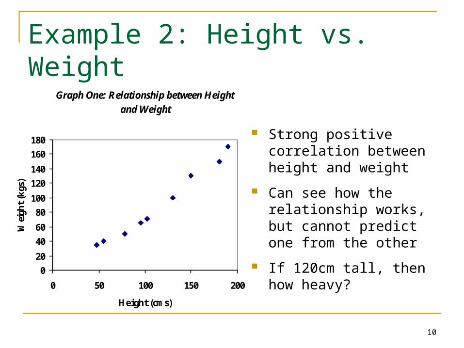
Example 2: Height vs. Weight
Graph One: Relationship between Height
and Weight
0
20
40
60
80
100
120
140
160
180
0 50 100 150 200
Height (cms)
Wei
ght
(kgs
)
Strong positive correlation between height and weight
Can see how the relationship works, but cannot predict one from the other
If 120cm tall, then how heavy?
11
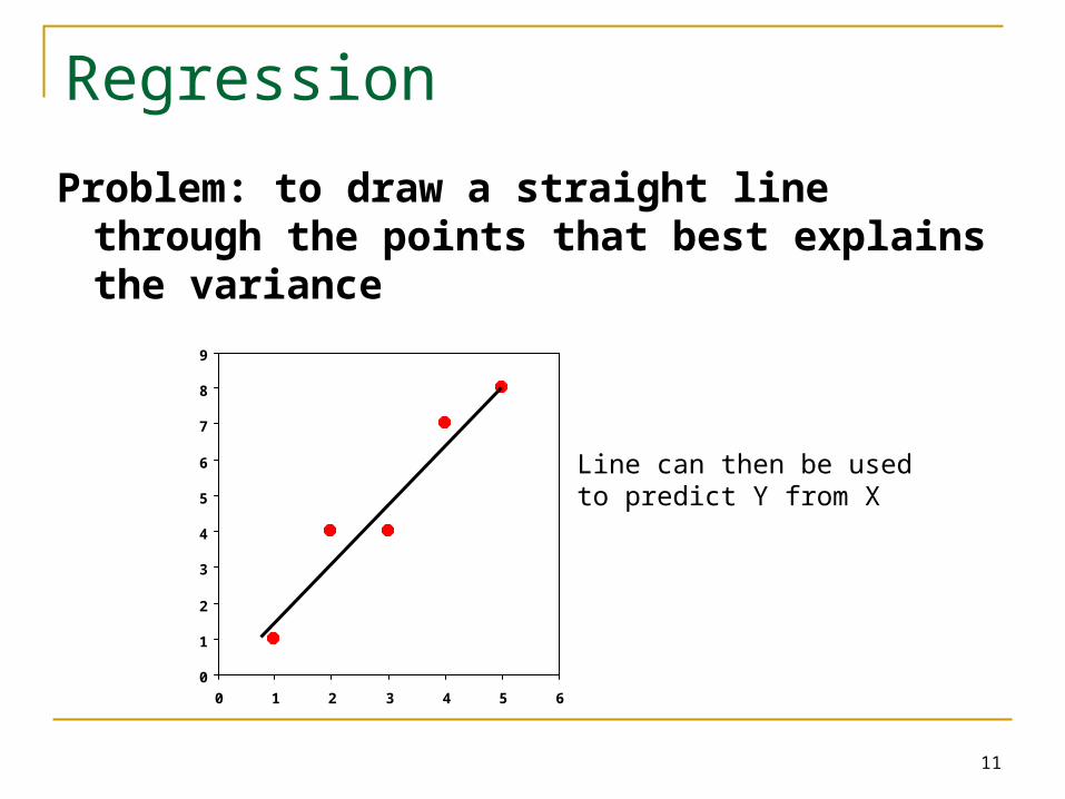
Problem: to draw a straight line through the points that best explains the variance
0
1
2
3
4
5
6
7
8
9
0 1 2 3 4 5 6
Regression
Line can then be used to predict Y from X
12
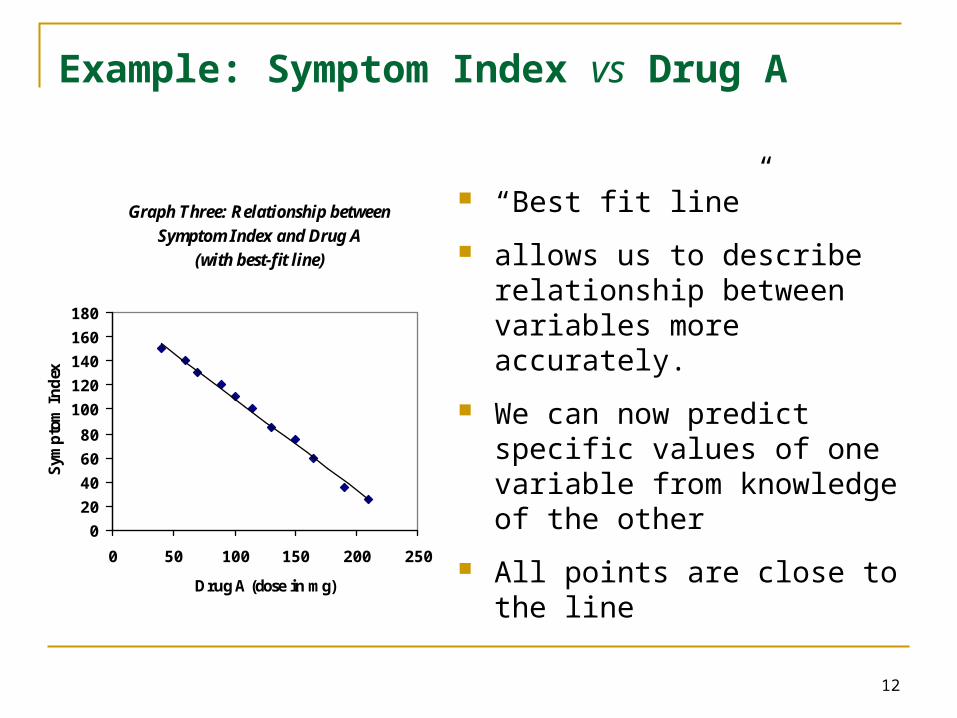
“Best fit line”
allows us to describe relationship between variables more accurately.
We can now predict specific values of one variable from knowledge of the other
All points are close to the line
Graph Three: Relationship between
Symptom Index and Drug A
(with best-fit line)
0
20
40
60
80
100
120
140
160
180
0 50 100 150 200 250
Drug A (dose in mg)
Sym
pto
m I
nd
exExample: Symptom Index vs Drug A
13
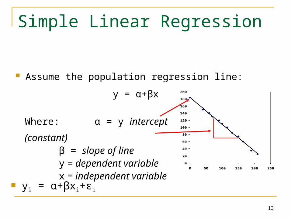
Assume the population regression line:
y = α+βx
0
20
40
60
80
100
120
140
160
180
200
0 50 100 150 200 250
Where: α = y intercept (constant) β = slope of line y = dependent variable x = independent variable
Simple Linear Regression
yi = α+βxi+εi
14
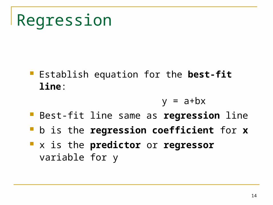
Establish equation for the best-fit line:
y = a+bx
Best-fit line same as regression line b is the regression coefficient for x x is the predictor or regressor variable for y
Regression
15
0
1
2
3
4
5
6
7
8
9
0 1 2 3 4 5 6
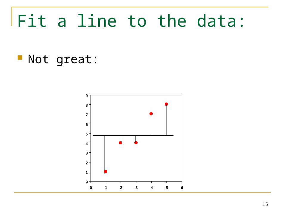
Fit a line to the data:
Not great:
16
0
1
2
3
4
5
6
7
8
9
0 1 2 3 4 5 6
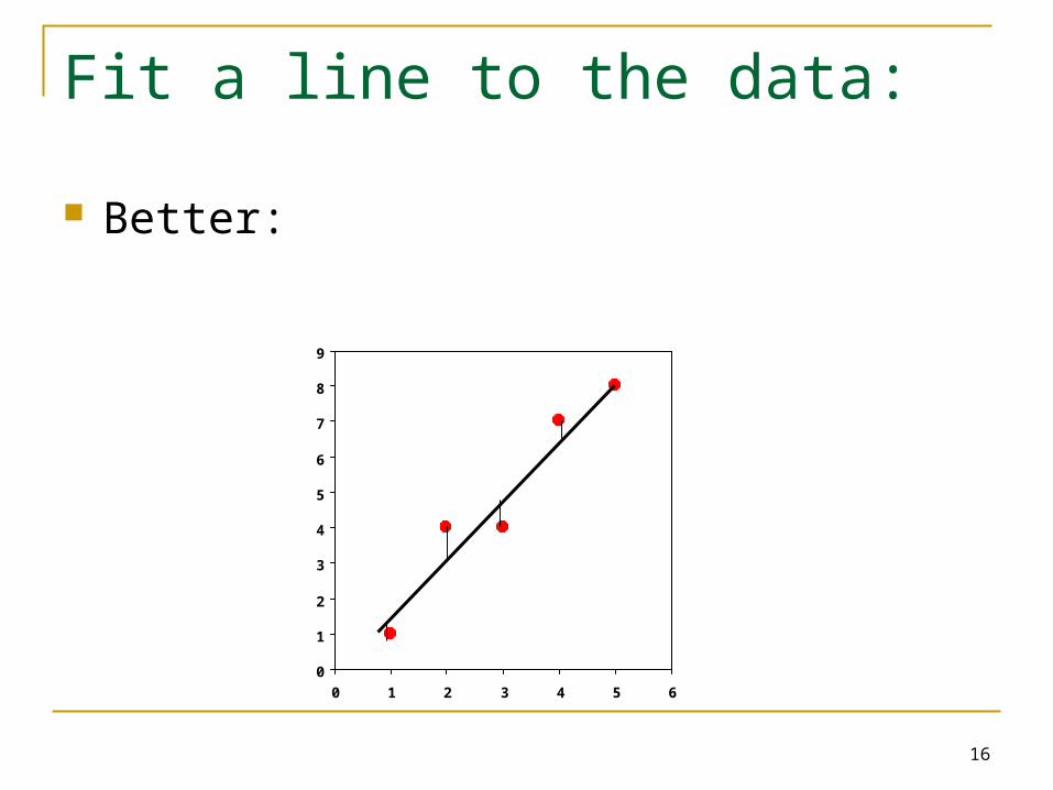
Fit a line to the data:
Better:

17
Least Squares
Minimise the (squared) distance between the points and the line a and b are the estimates of α and β which minimise
2)( ii xy
18
Least Squares Estimates
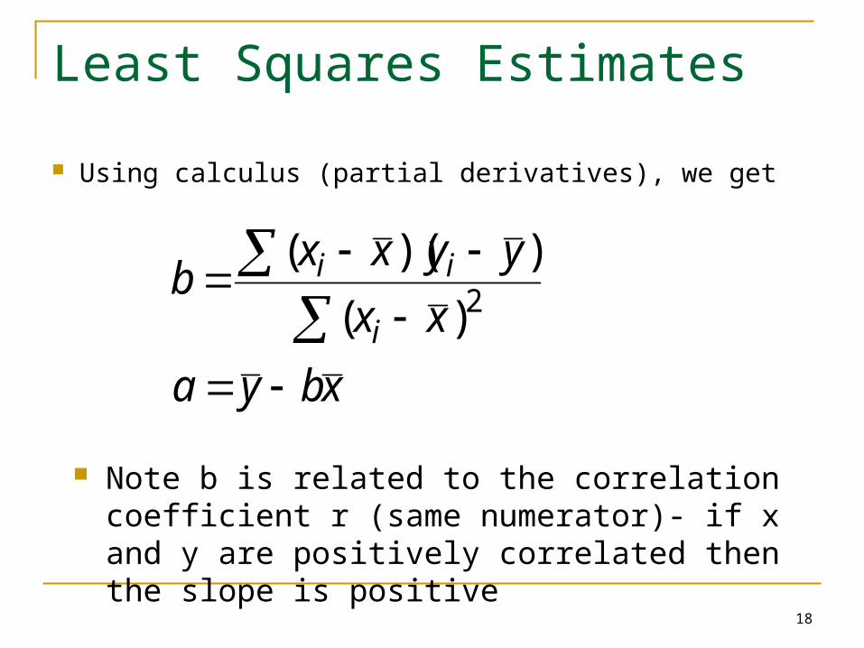
Using calculus (partial derivatives), we get
xbya
xx
yyxxb
i
ii
2)(
))((
Note b is related to the correlation coefficient r (same numerator)- if x and y are positively correlated then the slope is positive
19
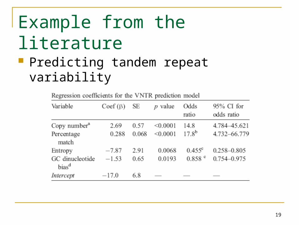
Example from the literature
Predicting tandem repeat variability
20
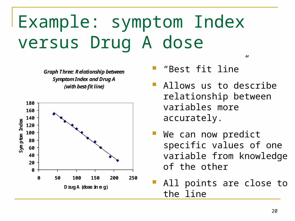
“Best fit line”
Allows us to describe relationship between variables more accurately.
We can now predict specific values of one variable from knowledge of the other
All points are close to the line
Graph Three: Relationship between
Symptom Index and Drug A
(with best-fit line)
0
20
40
60
80
100
120
140
160
180
0 50 100 150 200 250
Drug A (dose in mg)
Sym
pto
m I
nd
exExample: symptom Index versus Drug A dose
21
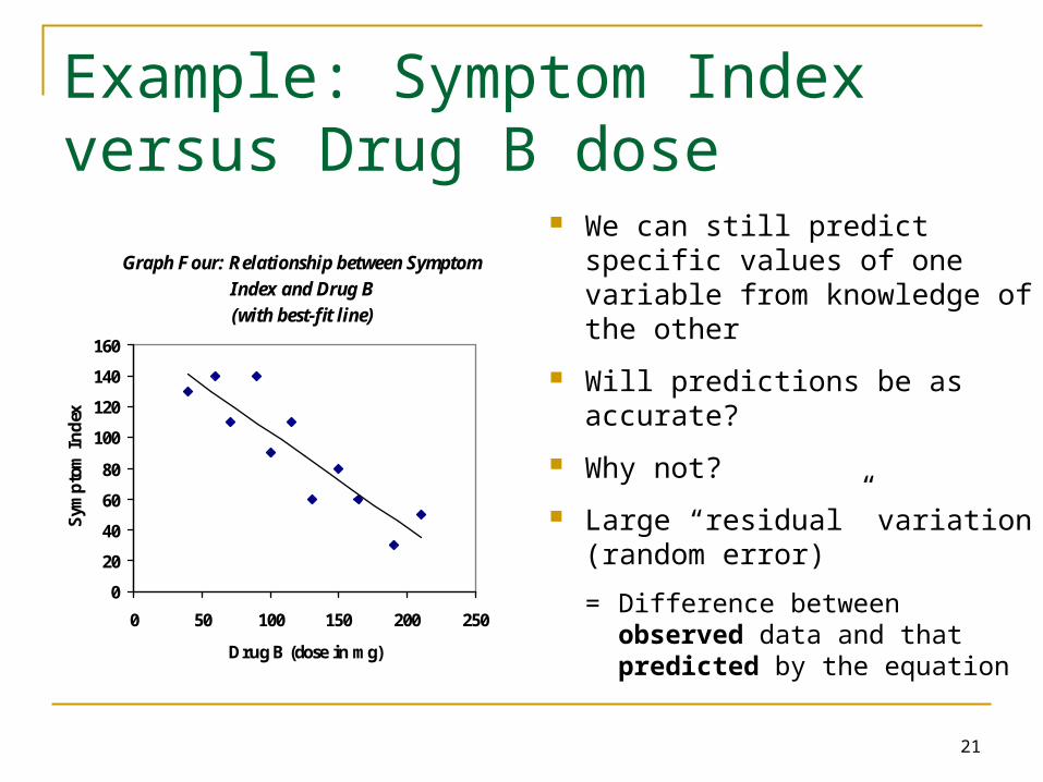
Graph Four: Relationship between Symptom Index and Drug B (with best-fit line)
0
20
40
60
80
100
120
140
160
0 50 100 150 200 250
Drug B (dose in mg)
Sym
pto
m I
nd
ex
We can still predict specific values of one variable from knowledge of the other
Will predictions be as accurate?
Why not?
Large “residual” variation (random error)
= Difference between observed data and that predicted by the equation
Example: Symptom Index versus Drug B dose
22
Regression Hypothesis Tests
Hypotheses about the intercept
H0: α = 0 HA: α 0
But most research focuses on the slope
H0: β = 0 HA: β 0
This addresses the general question “Is X predictive of Y?”
23
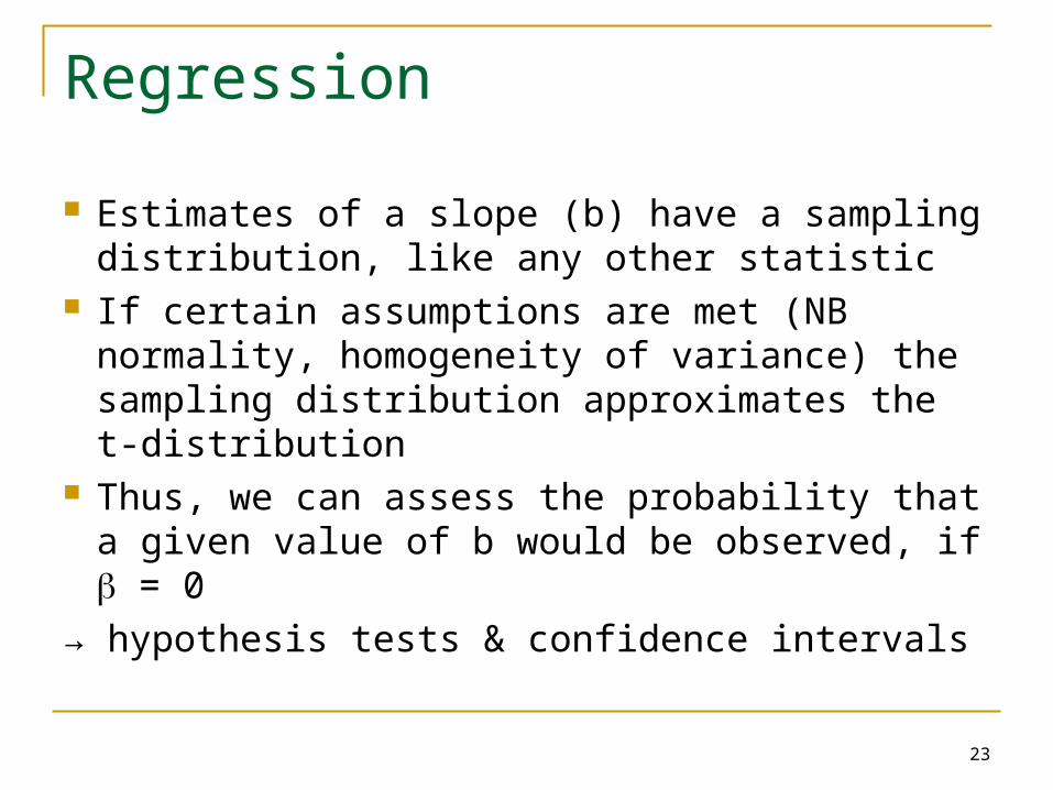
Regression
Estimates of a slope (b) have a sampling distribution, like any other statistic
If certain assumptions are met (NB normality, homogeneity of variance) the sampling distribution approximates the t-distribution
Thus, we can assess the probability that a given value of b would be observed, if = 0
→ hypothesis tests & confidence intervals

24
Regression R2, the coefficient of determination, is the percentage of variation
explained by the “regression”. R2 > 0.6 is deemed reasonably good. Note, the model must also be significant, e.g.

25
Back to SBP and Age example a=123 and b=0.159 approximately What does b mean? Is age predictive of BP? i.e. is there evidence
that b ≠ 0? How good is the fit of the regression line?
26
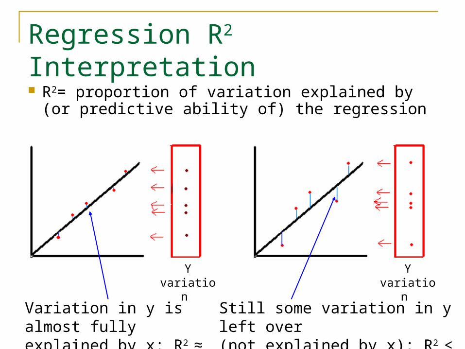
Regression R2 Interpretation
R2= proportion of variation explained by (or predictive ability of) the regression
Variation in y is almost fully explained by x: R2 ≈ 1
Still some variation in y left over(not explained by x): R2 < 1
Y variation Y variation

27
0
5
10
15
20
25
MEAN
REGRESSION LINE
{UNexplainederror
explainederror
TOTALerror

28
Regression – four possibilities
b ≠ 0P-value non-significant
b ≈ 0P-value non-significant
b ≠ 0P-value significant
b ≈ 0P-value significant
Relationship but not much evidence Plenty of evidence for a relationship
No relationship & not much evidence Plenty of evidence for no relationship
29
INCOME
100000800006000040000200000
HA
PP
Y
10
8
6
4
2
0
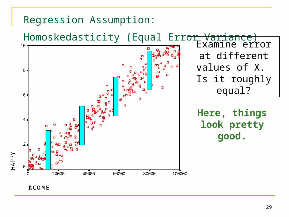
Regression Assumption:
Homoskedasticity (Equal Error Variance) Examine error at
different values of X. Is it roughly equal?
Here, things look pretty good.

30INCOME
100000
90000
80000
70000
60000
50000
40000
30000
20000
10000
0
HA
PP
Y
10
8
6
4
2
0
Heteroskedasticity: Unequal Error Variance
At higher values of X, error variance increases a lot.
A transformation of data (e.g. log)
can remove heterskedasticity
31
50% of slides complete!
32
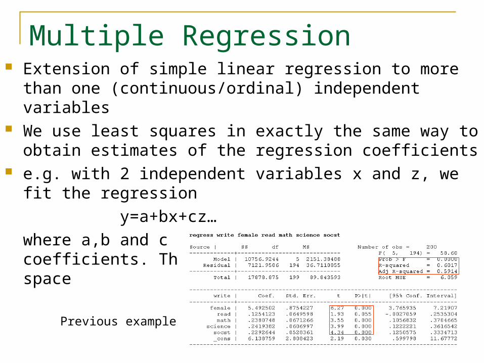
Multiple Regression Extension of simple linear regression to more than one
(continuous/ordinal) independent variables We use least squares in exactly the same way to obtain
estimates of the regression coefficients e.g. with 2 independent variables x and z, we fit the regression
y=a+bx+cz…
where a,b and c are the regression coefficients. This represents a plane in 3d space
Previous example

33
Notes on multiple regression
Make sure variables are normal. If not, transform them. If still not, can split into 2 groups (categories (0/1)) for e.g. high vs. low responders
Can combine with “stepwise selection”: instead of using every variable and forcing them into a final model, can drop out variables automatically, e.g. petri dish temperature, that are not predictive

34
Example
Study to evaluate the effect of the duration of anesthesia and degree of trauma on percentage depression of lymphocyte transformation
35 patients Trauma factor classified as 0, 1, 3 and 4,
depending upon severity

35
Duration Trauma Depression Duration Trauma Depression
4
6
1.5
4
2.5
3
3
2.5
3
3
2
8
5
2
2.5
2
1.5
1
3
3
2
2
2
2
2
2
3
3
3
3
4
2
2
2
2
1
36.7
51.3
40.8
58.3
42.2
34.6
77.8
17.2
-38.4
1
53.7
14.3
65
5.6
4.5
1.6
6.2
12.2
3
4
3
3
7
6
2
4
2
1
1
2
1
3
4
8
2
3
3
3
3
4
4
2
2
2
1
1
1
1
1
3
4
2
29.9
76.1
11.5
19.8
64.9
47.8
35
1.7
51.5
20.2
-9.3
13.9
-19
-2.3
41.6
18.4
9.9
36
Example (con’t)
Fitted regression line is
y=-2.55+10.375x+1.105zorDepression= -2.55+10.375*Trauma+1.105*Duration
Both slopes are non-significant (p-value=0.1739 for trauma, 0.7622 for duration)
R2=16.6% of the variation in lymphocyte depression is explained by the regression
Conclusion: Trauma score and duration of anesthesia are poor explanations for lymphocyte depression
37
Collinearity
If two (independent) variables are closely related its difficult to estimate their regression coefficients because they tend to get confused
This difficulty is called collinearity Solution is to exclude one of the highly
correlated variables
38
Example (cont’d)
Correlation between trauma and duration= 0.762 (quite strong)
Drop trauma from regression analysis
Depression=9.73+4.94*Duration
P-value for duration is 0.0457, statistically significant! However, the R2 is still small (11.6%) Conclusion: Although there is evidence for a non-zero slope
or linear relationship with duration, there is still considerable variation not explained by the regression.
39
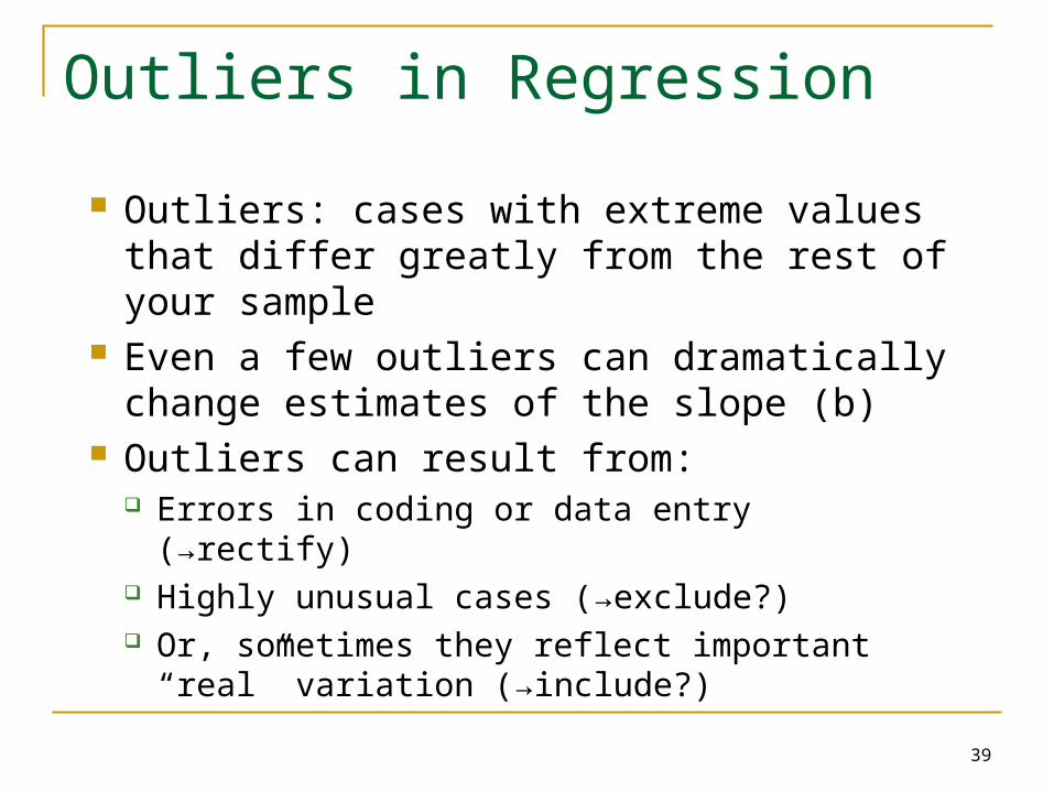
Outliers in Regression
Outliers: cases with extreme values that differ greatly from the rest of your sample
Even a few outliers can dramatically change estimates of the slope (b)
Outliers can result from: Errors in coding or data entry (→rectify) Highly unusual cases (→exclude?) Or, sometimes they reflect important “real”
variation (→include?)
40
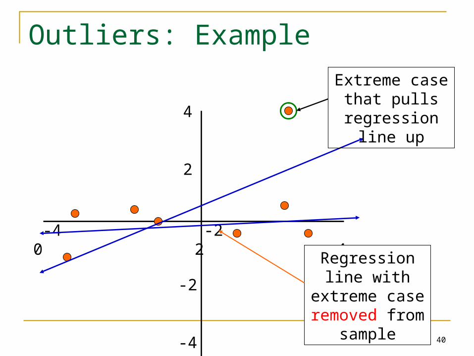
Outliers: Example
-4 -2 0 2 4
4
2
-2
-4
Extreme case that pulls regression
line up
Regression line with extreme case
removed from sample

41
Fail to reject β=0
Reject β=0
What about non-linear relationships?

42
Non-linear models
Linear Regression fits a straight line to your data Non-linear models may, in some cases, be more appropriate Non-linear models are usually used in situations where non-
linear relationships have some biological explanation e.g. non-linear models are commonly used in
pharmacokinetics studies and compartmental analysis Computationally intensive - estimates may not “converge”
and results may be difficult to interpret
43
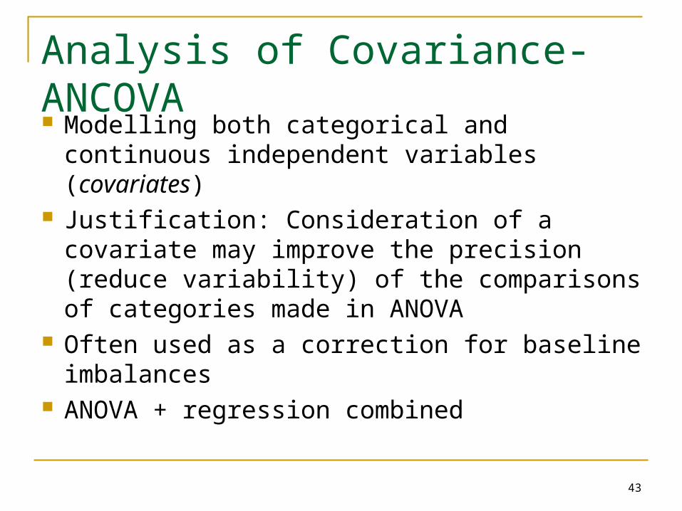
Analysis of Covariance-ANCOVA Modelling both categorical and continuous
independent variables (covariates) Justification: Consideration of a covariate
may improve the precision (reduce variability) of the comparisons of categories made in ANOVA
Often used as a correction for baseline imbalances
ANOVA + regression combined
44
45
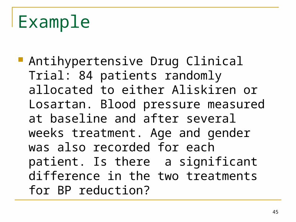
Example
Antihypertensive Drug Clinical Trial: 84 patients randomly allocated to either Aliskiren or Losartan. Blood pressure measured at baseline and after several weeks treatment. Age and gender was also recorded for each patient. Is there a significant difference in the two treatments for BP reduction?

46
Age Treatment Ba_daySBP Red_daySBP gender
66 SPP75 131.1 0.6 Female
62 SPP75 160.4 -0.7 Male
48 Los100 147.3 17.9 Male
32 Los100 144.8 -2.4 Male
61 Los100 150.7 21.6 Female
68 SPP75 152.4 6 Male
60 Los100 143.6 15.3 Male
33 SPP75 143.2 5.1 Male
69 Los100 166.6 24.6 Male
53 SPP75 147.6 Female
63 SPP75 163.7 -0.2 Male
64 Los100 145.7 15.5 Male
58 SPP75 168.3 0.5 Male
52 SPP75 156.8 0.6 Male
54 SPP75 154.9 7.3 Male
43 SPP75 170.5 -2.7 Female
46 SPP75 155.5 18.3 Female
46 Los100 173.1 26.7 Male
66 Los100 151.2 -1.7 Male
29 SPP75 139.8 -1.5 Male
50 SPP75 162.6 13 Male
49 SPP75 178.8 17.2 Female
40 SPP75 146.8 0 Male
52 Los100 157.1 -0.2 Female
68 Los100 152 8.9 Male
35 SPP75 145.4 2.8 Male
49 Los100 153.7 14.9 Male
47 SPP75 139.2 10 Male
Age Treatment Ba_daySBP Red_daySBP gender
45 Los100 156 17 Male
68 Los100 149.9 6.8 Female
48 Los100 147 16 Female
69 SPP75 145.3 -1.2 Male
64 Los100 142.5 20.6 Female
40 SPP75 168.6 2.6 Male
61 SPP75 165.6 8.1 Male
47 Los100 156.3 2.3 Female
60 Los100 147.7 11.5 Female
35 SPP75 157.4 12.5 Male
61 SPP75 143.7 -1.8 Male
62 Los100 148.6 6.6 Male
54 Los100 164.6 39.6 Female
45 Los100 145.3 -6.1 Female
57 SPP75 143.9 7 Female
48 SPP75 144.3 2.4 Male
59 Los100 147.8 1.1 Female
47 SPP75 150.4 -2.3 Male
54 Los100 143.9 -0.2 Male
45 SPP75 145.1 6.6 Male
61 SPP75 158 3 Male
69 Los100 154.8 Male
21 SPP75 142.1 Male
69 SPP75 171.3 -2 Male
66 Los100 140.3 2.8 Male
42 SPP75 146 5.7 Male
47 SPP75 159.3 14.6 Female
60 SPP75 157.8 6.8 Male
47
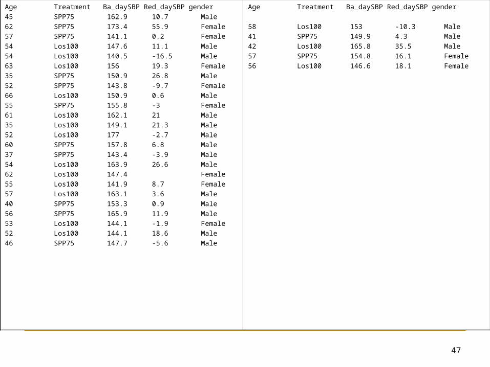
Age Treatment Ba_daySBP Red_daySBP gender
45 SPP75 162.9 10.7 Male
62 SPP75 173.4 55.9 Female
57 SPP75 141.1 0.2 Female
54 Los100 147.6 11.1 Male
54 Los100 140.5 -16.5 Male
63 Los100 156 19.3 Female
35 SPP75 150.9 26.8 Male
52 SPP75 143.8 -9.7 Female
66 Los100 150.9 0.6 Male
55 SPP75 155.8 -3 Female
61 Los100 162.1 21 Male
35 Los100 149.1 21.3 Male
52 Los100 177 -2.7 Male
60 SPP75 157.8 6.8 Male
37 SPP75 143.4 -3.9 Male
54 Los100 163.9 26.6 Male
62 Los100 147.4 Female
55 Los100 141.9 8.7 Female
57 Los100 163.1 3.6 Male
40 SPP75 153.3 0.9 Male
56 SPP75 165.9 11.9 Male
53 Los100 144.1 -1.9 Female
52 Los100 144.1 18.6 Male
46 SPP75 147.7 -5.6 Male
Age Treatment Ba_daySBP Red_daySBP gender
58 Los100 153 -10.3 Male
41 SPP75 149.9 4.3 Male
42 Los100 165.8 35.5 Male
57 SPP75 154.8 16.1 Female
56 Los100 146.6 18.1 Female
48
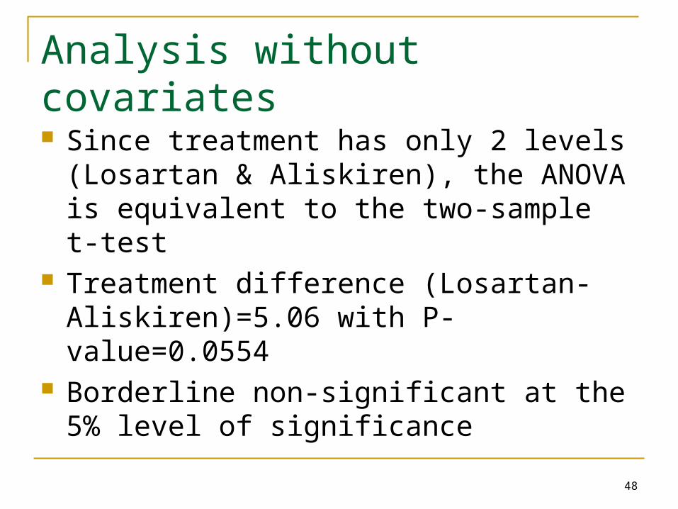
Analysis without covariates
Since treatment has only 2 levels (Losartan & Aliskiren), the ANOVA is equivalent to the two-sample t-test
Treatment difference (Losartan-Aliskiren)=5.06 with P-value=0.0554
Borderline non-significant at the 5% level of significance
49
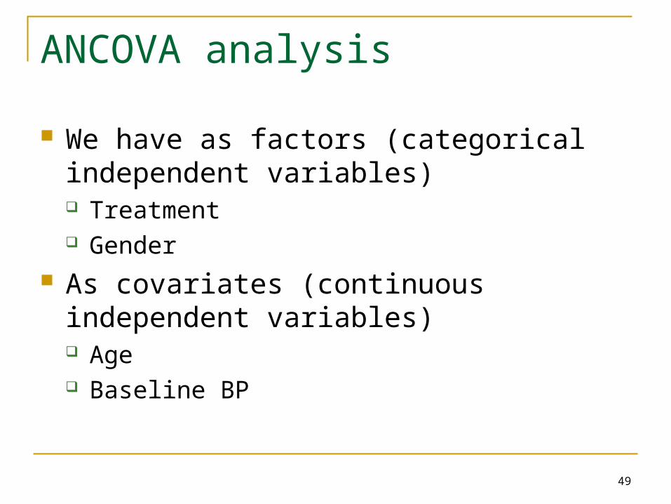
ANCOVA analysis
We have as factors (categorical independent variables) Treatment Gender
As covariates (continuous independent variables) Age Baseline BP
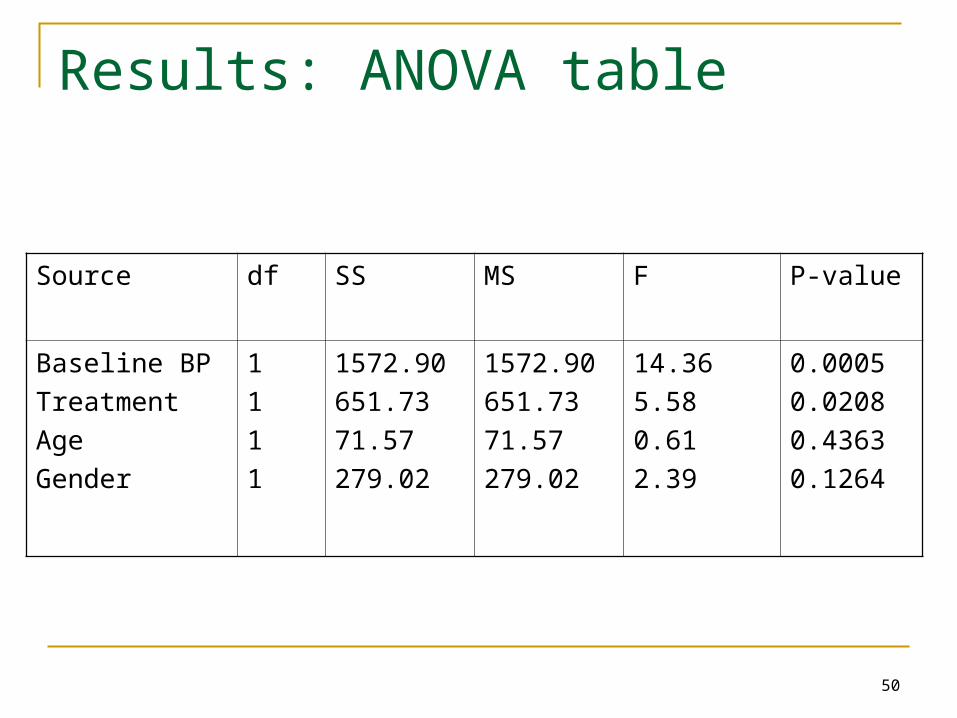
50
Results: ANOVA table
Source df SS MS F P-value
Baseline BP
Treatment
Age
Gender
1
1
1
1
1572.90
651.73
71.57
279.02
1572.90
651.73
71.57
279.02
14.36
5.58
0.61
2.39
0.0005
0.0208
0.4363
0.1264
51
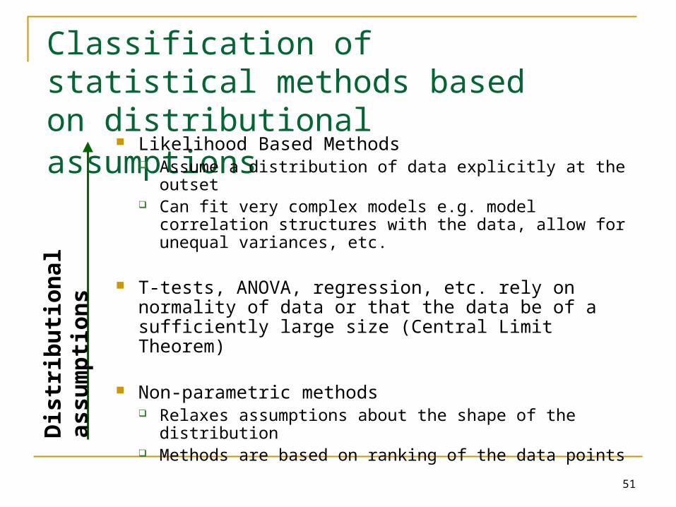
Classification of statistical methods based on distributional assumptions
Likelihood Based Methods Assume a distribution of data explicitly at the outset Can fit very complex models e.g. model correlation
structures with the data, allow for unequal variances, etc.
T-tests, ANOVA, regression, etc. rely on normality of data or that the data be of a sufficiently large size (Central Limit Theorem)
Non-parametric methods Relaxes assumptions about the shape of the distribution Methods are based on ranking of the data points
Dis
trib
uti
on
al a
ssu
mp
tio
ns
52
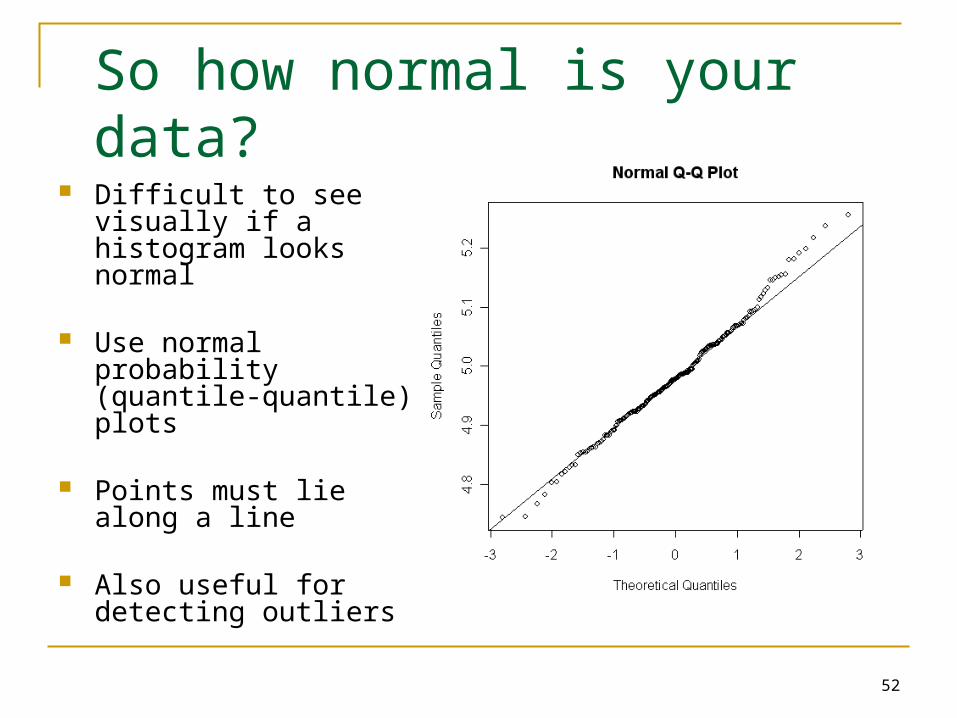
So how normal is your data?
Difficult to see visually if a histogram looks normal
Use normal probability (quantile-quantile) plots
Points must lie along a line
Also useful for detecting outliers

53
Significant Deviations from Normality: Alternatives Transform your data to make it more “normal” and
use standard parametric tests e.g. log transform (eliminates skew) Difficulty - may wish to reverse-transform results
back (e.g. exponentiate parameter estimates)
Use non-parametric methods Make less assumptions on distribution shape These may have less power than parametric
methods

54
Non-parametric Equivalents
Parametric Non-parametric
Paired T-test
Two-sample T-test
ANOVA
Pearson’s Correlation
ANCOVA
Wilcoxon Signed Rank Test
Wilcoxon Rank-Sum
Kruskal Wallis Analysis
Spearman’s Rank Correlation
ANCOVA on ranked data
55
Other Multivariate Methods
Multivariate Analysis of Variance (MANOVA) ANOVA with more than one dependent variable or response Also MANCOVA Low power is a problem Not so widely used
The objectives behind multivariate analyses can be quite different (to those presented), namely Discriminant Analysis Classification Clustering Pattern Recognition (principal components analysis)
56
Sample Size Calculations
How many observations are needed in a study?
No mystery to this: sample sizes are often calculated by inverting the computations involved in determining statistical significance
Unfortunately, several quantities are required before we can do any calculations (and the argument is a little circular!)

57
Need to specify:
Study design and statistical test to be used e.g. we wish to compare 2 treatments, use the two-
sample t-test, two-tailed
Level of significance α (usually 0.05 i.e. 5%) Power β (commonly set to 0.80)
But we also need (with more difficulty): Difference we would like to detect? An estimate of the variability σ2 one expects to see in
the data?
58
Example: Two-sample t-test
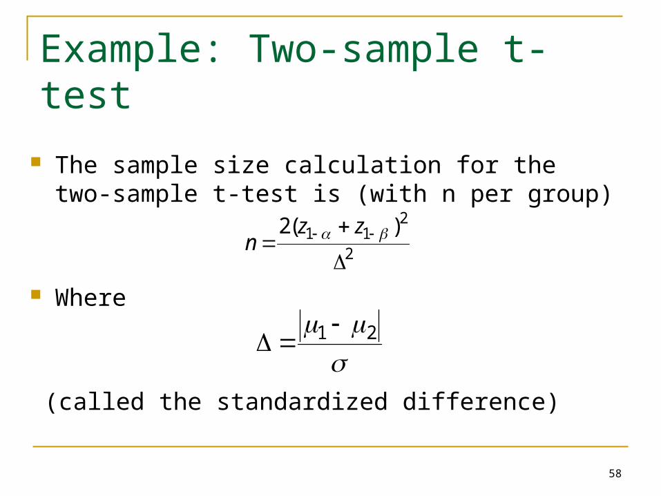
The sample size calculation for the two-sample t-test is (with n per group)
Where
(called the standardized difference)
2
211 )(2
zz
n
21

59
Example: Two-sample t-test calculation
In order to detect a standardised difference of 0.3 at the 5% level of significance (one-tail) and 80% power (z0.95=1.645, z0.80=0.84), we need a sample size of 138 per group.
60
Recommended Books/Links
“Statistical Methods in Medical Research” by Armitage, Berry, Matthews (4th edition, 2002). Oxford, Blackwell Science
“Practical Statistics for Medical Research” by Altman (1999). Kluwer Academic Publishers#
Statnotes: Topics in Multivariate Analysis, by G. David Garson: http://www2.chass.ncsu.edu/garson/PA765/statnote.htm
Statistical computing resources – UCLA: http://www.ats.ucla.edu/stat/
61
Statistics Software
Excel stats add-in is not recommended Stats calculations cannot be trusted (e.g. standard deviations
may be inaccurate) Doesn’t have the functionality of other software
STATA, S-Plus, Minitab, SAS, JMP, SPSS, R Certain amount of programming skill required but well worth it R is free; SAS is most expensive (up to 10k per person per
annum)
DataDesk, InStata –user friendly. “point-and-click”, with reasonable functionality