Boğaziçi UniversityDepartment of Management Information Systems

MIS 463 Decision Support Systems for Business

PROJECT FINAL

SALES FORECASTING SYSTEM

Project Team No: 10

Jung, PhilippKeskin, Uğur

Kılıç, Recep SonerKodaz, NebileUsta, Murat

Instructor : Aslı Sencer

İstanbul - December, 2013

Table of Contents1. INTRODUCTION.........................................................................................................3

1.1 THE DECISION ENVIRONMENT.......................................................................31.1.1 FORECASTING ERRORS..............................................................................3

1.2 MISSION OF THE PROJECT................................................................................41.3 SCOPE OF THE PROJECT....................................................................................41.4 METHODOLOGY..................................................................................................4

2. LITERATURE SURVEY.............................................................................................52.1 WHAT IS DSS?......................................................................................................52.2 THE NEED OF DSS IN SALES FORECASTING AND ITS STEPS...................5

2.2.1 EIGHT STEPS TO FORECASTING...............................................................62.3 WHY EXPONENTIAL SMOOTHING?................................................................6

2.3.1 EXPONENTIAL SMOOTHING HISTORY/SUMMARY.............................72.4 DEVELOPMENT OF TIME SERIES FORECASTING........................................7

2.4.1 Brief History of Forecasting.............................................................................72.4.2 Need for Forecasting........................................................................................82.4.3 Types of Forecasts............................................................................................8

3. DEVELOPMENT OF THE DSS................................................................................143.1 DSS ARCHITECTURE........................................................................................143.2 TECHNICAL ISSUES..........................................................................................143.3 MODELS...............................................................................................................14

3.3.1 VARIABLES..................................................................................................143.3.2 SINGLE EXPONENTIAL SMOOTHING....................................................153.3.3 DOUBLE EXPONENTIAL SMOOTHING..................................................193.3.4 TRIPLE EXPONENTIAL SMOOTHING.....................................................22

3.4 ALGORITHM.......................................................................................................303.5 USER INTERFACES AND REPORTS...............................................................31

4. ASSESSMENT...........................................................................................................425. PROJECT PLAN.........................................................................................................436. CONCLUSION...........................................................................................................447. REFERENCES............................................................................................................44

2

1. INTRODUCTION

1.1 THE DECISION ENVIRONMENT

The aim of the Sales Forecasting System is to predict the next year’s sales on a monthly basis for the next year by using the sales data of the recent year.

Every company that uses sales forecasts possesses its own technique to approach the forecasting process. Some companies have a dedicated team of forecast professionals while others use the sales staff to generate the forecast. The statistical methods used to generate the sales forecast depend on the demand profile of the product. Statistical forecast methods vary widely and finding the right method often boils down to trial and error.

In order to forecast the sales, companies use both quantitative and qualitative techniques. However, most companies use quantitative techniques since quantitative data is more reliable and helps to draw logical conclusions. In order to carry out reliable forecasts, the method called “exponential smoothing” is commonly used by wide range of companies around the globe.

The purpose of this project is to forecast the sales of next year in order to be able to plan inventory management, to retrieve customer information and allocate the staff properly.More precise Inventory Management helps controlling the inventory in a more efficient way. It can do so by examining trends showing the peak of sales or slow selling periods. This will prevent losses related to the sales that are not realized and save costs.

According to buying patterns of each customer the Sales Forecasting System spots the trends. Data related to these trends is going to help the company to keep track of each individual customer and sell them products that are beneficial for them. It also helps to identify the products that are purchased frequently by a customer in order to make special offers increasing sales.

Sales Forecasting System supports adequate staffing. Through the data gained, peaking sales as well as decrease in sales can be anticipated. So either additional employees can be hired or working hours can be reduced to an efficient level.

All in all the Sales Forecasting System improves the factors mentioned above and leads to competitive advantages such as the minimization of costs, the increase in sales and customer satisfaction.

1.1.1 FORECASTING ERRORS

Possible reasons for errors in forecasting Flows in data used in forecasting process Insufficient data Unpredictable economic and socio-political environment Non-realistic and accurate assumptions Technical and technological changes Shifts in economic structure Administrative errors

3

1.2 MISSION OF THE PROJECT

The mission is to provide analyzed and summarized sales forecasting report to related managerial level by using historical sales data.

With that system, the forecasting specialists, just by getting the historical data set and setting some constant(s), could prepare desired reports. This is a time-efficient method, especially when the large companies’ operations come into question.

The project’s other mission is to support other departments’ critical works. The Human Resources Department, for instance, can take this report as a reference while scheduling the employee numbers of stores. The Inventory Management Department can also take this report into account in order to determine each store’s physical stock amount and related space in the stock room of the store itself. The Customer Information Service plays significant role in sales. If the forecast shows that there will be a negative trend in the sales, this service immediately sets some events such as promotions, small gifts, and/or significant discount rates, and inform the customers in the way that they normally use.

Goal: Providing the sales forecasting report which is requested by supervisors or managers. According to that report the managers occasionally take actions regarding their department works.

1.3 SCOPE OF THE PROJECT

The forecasting specialists, after getting the historical data set which is our main input, enter the required constant value(s), for instance, α for exponential smoothing and α and β constants together for double exponential smoothing. Then the system retrieves the forecasting report for the next periods and also sketches corresponding graphical illustrations.

By taking this report into account, some other departments such as Human Resources Department could go in for changes in staff amount in stores, but that report/project is not directly responsible for or a part of these departments’ internal operations.

1.4 METHODOLOGY

For a decision support system, using the right methodology is quite important. With the right methodology, it will be easy to model. Besides, the problem itself requires an appropriate methodology to be solved easily and in an efficient way. Considering all these, we have chosen to use Exponential Smoothing method as our methodology. The reason why we have chosen this methodology is that exponential smoothing forecasts demand in the next period by taking into account the actual demand in the current period and the forecast which was previously made for the current period.

The program uses the historical sales data which is obtained from Turkish Head Office of Inditex Group for the company’s flagship brand of ZARA.

4

2. LITERATURE SURVEY

2.1 WHAT IS DSS?

DSS was first stated as “Management Decision Systems” in the early 1970s by Michael S. Scott Morton (Morton, 1971). As a few firms and a few scholars began to develop this area of research, the term “Decision Support Systems” became current. “DSS became characterized as interactive computer-based systems which help decision makers utilize data and models to solve complex problems.” (Fick & Sprague & Editors, 1980)

Since the early 1970s, DSS technology and applications have evolved significantly. Many technological and organizational developments have contributed to this evolution. DSS once utilized more limited database, modeling, and user interface functionality, but technological innovations have enabled far more powerful DSS functionality. For example; DSS is enable to generate some reports. This functionality is now a common feature used to present the results to the user in a form which can be very practical for him and also can be integrated into databases. Solutions can also be stored in popular spreadsheet formats for simple graphical analyses or report generation (Shim& Warkentin & Courtney& Power& Sharda, Carlsson, 2002). DSS provides many benefits to the user in that it gives reasonable and measurable outcome with a better decision making process taking into account uses of the computerized world. However in some cases both the outcome and process is not affected. Even in this case DSS is beneficial because it provides documentation of quality of the processes in that the stakeholders can be convinced of correcting their decisions (Burstein & Holsapple, 2008).

Modern decisions support systems provide many capabilities to the user with the development in technology. The global Internet and the World Wide Web are now the primary enabling technologies for delivering computerized decision support. Many firms use the Web as a medium to convey information about DSS products or to distribute DSS software (Bhargava & Power & Sun, 2007). Companies are creating Web based DSS which customers can use these systems to evaluate products or suppliers can used to control cost or reduce inventories (Power & Kaparthi, 2002).

Due to the growing interest in the Web, there are many on-going efforts to develop and implement Web-based DSS in various areas, such as health care, private companies, government, and education (Bhargava &Power & Sun, 2007). The project that we are carrying out is focused on sales forecasting.

2.2 THE NEED OF DSS IN SALES FORECASTING AND ITS STEPS

Sales forecasting always plays a prominent role in a decision support system. Obtaining effective sales forecasting in advance can help the decision maker calculate production and materials costs, even determine the sale price. This will result in a lower inventory level and achieve the objective of just-in-time (Kuo & Xue, 2012).

Every day, managers make decisions without knowing what will happen in the future. Inventory is ordered though no one knows what sales will be, new equipment is

5

purchased though no one knows the demand for products, and investments are made though no one knows what profits will be. Managers are always trying to reduce this uncertainty and to make better estimates of what will happen in the future. Accomplishing this is the main purpose of forecasting.

There are many ways to forecast the future. In numerous firms (especially smaller ones), the entire process is subjective, involving seat-of-the-pants methods, intuition, and years of experience. There are also many quantitative forecasting models, such as moving averages, exponential smoothing, trend projections, and least squares regression analysis.

The following steps can help in the development of a forecasting system. While step 5 and 6 may not be as relevant if a quantitative model is selected in the step 4, data are certainly necessary for the quantitative forecasting models.

2.2.1 EIGHT STEPS TO FORECASTING

1- Determine the use of the forecast – what objective are we trying to obtain?2- Select the items or quantities that are to be forecasted.3- Determine the time horizan of the forecast – is it 1 to 30 days (short term), 1

month to 1 year (medium term), or more than 1 year (long term)?4- Select the forecasting model or models.5- Gather the data or information needed to make the forecast.6- Validate the forecasting model.7- Make the forecast.8- Implement the results.

These steps present a systematic way of initiating, designing, and implementing a forecasting system. When the forecasting system is to be used to generate forecasts regularly over time, data must be collected routinely, and the actual computations or procedures used to make the forecast can be done automatically (Render, Stair & Hanna, 2012).

There is seldom a single superior forecasting method. One organization may find regression effective, another firm may use several approaches, and a third may combine both quantitative and subjective techniques. Whatever tool works best for a firm is the one that should be used (Render, Stair & Hanna, 2012). In this project, we use the exponential smoothing (single, double, and triple) method.

2.3 WHY EXPONENTIAL SMOOTHING?

Exponential smoothing schemes weight past observations using exponentially decreasing weights.

This is a very popular scheme to produce a smoothed time series. Whereas in single moving averages the past observations are weighted equally, exponential smoothing assigns exponentially decreasing weights as the observation get older.

6

In other words, recent observations are given relatively more weight in forecasting than the older observations.

In the case of moving averages, the weights assigned to the observations are the same and are equal to 1/N. In exponential smoothing, however, there are one or more smoothing parameters to be determined (or estimated) and these choices determine the weights assigned to the observations (Nist / Sematech, 2013).

Single, double and triple exponential smoothing will be described in the model and algorithm section.

2.3.1 EXPONENTIAL SMOOTHING HISTORY/SUMMARY

Exponential smoothing has proven through the years to be very useful in many forecasting situations. It was first suggested by C.C. Holt in 1957 and was meant to be used for non-seasonal time series showing no trend. He later offered a procedure (1958) that does handle trends. Winters (1965) generalized the method to include seasonality, hence the name "Holt-Winters Method".

The Holt-Winters Method has 3 updating equations, each with a constant that ranges from 0 to 1. The equations are intended to give more weight to recent observations and less weight to observations further in the past. These weights are geometrically decreasing by a constant ratio (Nist / Sematech, 2013).

Please check the next section for more detailed information about exponential smoothing.

2.4 DEVELOPMENT OF TIME SERIES FORECASTING

2.4.1 Brief History of Forecasting

Many of the forecasting techniques used today were developed in 19th century. There are great deals of issues whose results can now be forecasted easily. For example, sunrise can be predicted, as can the speed of a falling object, the onset of hunger, thirst or fatigue, rainy weather, and a number of other events. However, that was not always the case.

By the evolution of science it is now possible to understand various aspects of an environment than it could be in the past. As a result, this increased understanding brought predictability of many events. For instance, by development of Ptolemaic system of astronomy nineteen hundred years ago, it became possible to predict the movement of any star with accuracy unheard of before that time. With emergence of Copernican astronomy the predictions became even more accurate. Today’s modern astronomy is far more accurate than Copernican astronomy (Makridakis, 1978).

With the development of more sophisticated forecasting techniques, along with the advent of computers, forecasting has received more and more attention. Today it is inevitable for managers to use forecasting technique in order to make decisions about future of the organization. The need for forecasting is increasing as management

7

attempts to decrease its dependence on chance and becomes more scientific in dealing with its environment.

New techniques for forecasting continue to be developed as management concern with the forecasting process continues to grow.

2.4.2 Need for Forecasting

With globalization business environment became even more competitive than it ever was before. In order to survive in such environment organizations need to make their decision not solely on judgmental elements but derive their decisions from more concrete and reliable data. Forecasting is the best way to make decisions about future as long as the data being used is relevant and reliable. Any lapse in choosing the data which will be used in the forecast might cause great losses for organizations. If everything was constant in the world we are living, there would be no need for forecasting. Since the world in which organizations operate is steadily changing, forecasts will always be necessary. For example, the sales of a company are not the same for each month, quarter or year. Forecasting is not only needed by international, large companies but also by small companies as well since almost every organization must plan to meet conditions of the future for which it has imperfect knowledge. Forecasts are needed in finance, marketing, personnel, and production areas, in government and profit-seeking organizations, in small social clubs, and in national political parties (Hanke & Wichern & Reitsch, 2001).

2.4.3 Types of Forecasts

Generally, two types of data are of interest for forecasters. The first are data collected at a single point in time, be it an hour, a day, a week, a month, or a quarter. The second are observations of data made over time. When all observations are from the same time period, they are called cross-sectional data. The objective is to examine such data and then to extrapolate or extend the revealed relationships to the larger population (Hanke & Wichern & Reitsch, 2001). Drawing a random sample of personnel files to study the circumstances of the employee of a company is one example. Any variable that consists of data that are collected, recorded, or observed over successive increments of time is called time series. Monthly sales of a company are an example of time series (Makridakis, 1978).

Since our project includes time series data, only the methods of forecasting related to time series data will be discussed in this session.

2.4.3.1 Naïve Models

This model is being used mostly by young businesses. Since most forecasting methods require large amount of data, it is not possible to make forecasting for young businesses since they have very small data sets. Naïve forecasts are one possible solution since they

8

are based solely on the most recent information available (Hanke & Wichern & Reitsch, 2001). Naïve forecasts assume that recent periods are the best predictors of the future.The simplest model is

Ŷt+1 = Ytwhere Ŷt+1 is the forecast made at time t for time t+1.

The naïve forecast for each period is the immediately preceding observation. One hundred percent of the weigh is given to the current value of the series.

Since the naïve forecast discards all other observations, this scheme tracks changes very rapidly. The problem with this approach is that random fluctuations are tracked as faithfully as any other model changes.

The major weakness of naïve approach is that it ignores everything that has occurred since last year and also any trending. There are several ways of introducing more recent information.

It is apparent that number and complexity of possible naïve models are limited only by the ingenuity of the analyst, but use of these techniques should be guided by sound judgment.

2.4.3.2 Forecasting Methods Based on Averaging

Frequently, management faces the situation in which forecasts need to be updated daily, weekly, or monthly for inventories containing hundreds or thousands of items. Often it is not possible to develop sophisticated forecasting techniques for each item. Instead, some quick, inexpensive, very simple short-term forecasting tools are needed to accomplish this task.

A manager facing such a situation is likely to use an averaging or smoothing technique. These types of techniques use a form of weighted average of past observations to smooth short-term fluctuations. The assumption underlying these techniques is that the fluctuations in past values represent random departures from some smooth curve. Once this curve is identified, it can be projected into the future to produce a forecast (Hanke & Wichern & Reitsch, 2001).

2.4.3.2.1 Simple Averages

As with the naïve methods, a decision is made to use the first t data points as the initialization part and the rest as a test part. Next, the equation below is used to average the initialization part of the data and to forecast the next period.

Ŷt+1 =1t ∑i=1

t

Y i

9

The method of simple averages is an appropriate technique when the forces generating the series to be forecast have stabilized, and the environment in which the series exists is generally unchanging. Examples of this type of series are the quantity of sales resulting from a consistent level of salesperson effort; the quantity of sales of a product in the mature stage of its life cycle; and number of appointments per week requested of a dentist, doctor, or lawyer whose patient base is fairly constant.

2.4.3.2.2 Moving Averages

A constant number of data points can be specified at the outset and a mean computed for the most recent observations. The term moving average is used to describe this approach. As each new observation becomes available, a new mean is computed by adding the newest value and dropping the oldest. The equation below gives the simple moving average model. A moving average of order k, MA(k), is computed by

Ŷ t+1.=

(Y t+Y t−1+Y t−2+…+Y t−k+1)k

where

Ŷt+1 = forecast value for next periodYt = actual value at period tk = number of terms in the moving average

In this case equal weights are assigned to each observation. Each new data point is included in the average as it becomes more available, and the earliest data point is discarded.

This technique deals only with the latest k periods of known data; the number of data points in each average does not change as time continues. The model does not handle trend and seasonality very well, although it does better than the simple average method.For quarterly data, a four quarter moving average, MA(4), yields an average of the four quarters, and for monthly data, a MA(12), eliminates or averages out seasonal effects. The larger the order of the moving average, the greater the smoothing effect.

2.4.3.3 Exponential Smoothing Methods

2.4.3.3.1 Single Exponential Smoothing

Whereas the method of moving averages only takes into account the most recent observations, simple exponential smoothing provides an exponentially weighted moving average of all previously observed values. The model is often appropriate for data with no predictable upward or downward trend.

This method is based on averaging past values of a series in a decreasing (exponential) manner. The observations are weighted, with more weight being given to the more recent observations (Corberán-Vallet, Bermúdez, Vercher, 2011).

10

The smoothing constant α serves as the weighting factor. The actual value of α determines the extent to which the current observation is to influence the forecast value. When α is close to one, the new forecast will include substantial adjustment for any error that occurred in the preceding forecast. Conversely, when α is close to zero, the new forecast will be very similar to the old one (Hanke & Wichern & Reitsch, 2001).

If it is desired that predictions be stable and random variations smoothed, a small value of α is required. If a rapid respond to a real change in the pattern of observations is desired, a larger value of α is appropriate.

An assumption of the simple exponential smoothing technique is that the data vary about a level those changes infrequently. Whenever a significant trend exists, simple exponential smoothing will lag behind the actual values over time (Hanke & Wichern & Reitsch, 2001).

2.4.3.3.2 Exponential Smoothing Adjusted for Trend: Holt’s Method (Double Exponential Smoothing)

In simple exponential smoothing the level of the times series is assumed to be changing occasionally and an estimate of the current level is required. In some situations, the observed data will be trending and contain information that allows the anticipation of future upward movements. When this is the case, a linear trend forecast function is needed. Holt (1957) developed an exponential smoothing method, Holt’s two parameter method, which allows for evolving local linear trends in a time series.

When upward movement in the time series is anticipated, and estimate of the current slope, as well as the current level, is required. Holt’s technique smoothes the level and slope directly by using different smoothing constants for each (α and β). These smoothing constants provide estimates of level and slope that adapt over time as new observations become available. One of the advantages of Holt’s technique is that it provides a great deal of flexibility in selecting the rates at which the level and trend are tracked.

As with simple exponential smoothing, the weights α and β can be selected subjectively or by minimizing a measure of forecast error such as the MSE. Large weights result in more rapid changes in the component; small weights result in less rapid changes. Therefore, the larger the weights the more the smoothed values follow the data; the smaller the weights the smoother the pattern in the smoothed values.

The large amount of error indicates that possibility of seasonal variation in the data needs to be investigated.

2.4.3.3.3 Exponential Smoothing Adjusted For Trend and Seasonal Variation: Winter’s Method (Triple Exponential Smoothing)

Winter’s (1960) three-parameter linear and seasonal exponential smoothing model, an extension of Holt’s model, might reduce forecast error. One additional equation is used to estimate seasonality. This seasonality is given as seasonal index.

11

Winter’s method provides an easy way to explain the seasonality in a model when data have a seasonal pattern.

2.4.3.4 Autoregressive Moving Average (ARMA) Model

In the statistical analysis of time series, autoregressive moving average (ARMA) models provide a parsimonious description of a (weakly) stationary stochastic process in terms of two polynomials, one for the auto-regression and the second for the moving average. In this model there is a stationary part by autoregressive model and there is a randomness in a specific band width by moving average model. The ARMA model is a univariate model. In the model the error term is white noise error. ARMA is appropriate when a system is a function of a series of unobserved shocks (the MA part) as well as its own behavior. For example, stock prices may be shocked by fundamental information as well as exhibiting technical trending and mean-reversion effects due to market participants. The ARMA model is a univariate model (De Gooijer & Hyndman, 2006).

2.4.3.5 Autoregressive Integrated Moving Average (ARIMA)

It integrates aoutoregressive method and moving average method. The ARIMA model also uses the time series as exponential smoothing model. The time series are polinomial functions plus white noise. In the ARIMA model the error rate can be estimated. Inputs can have missing values and outliers. To have beter forecasting results, these outliers should be aggregated. Box-Jenkins parameter optimization technique is used in ARIMA (Stepnicka & Cortez & Donate & Stepnicka, 2013).

There are some variations on the ARIMA model. If multiple time series are used then the variables can be thought of as vectors and a VARIMA model may be appropriate. Sometimes a seasonal effect is suspected in the model; in that case, it is generally better to use a SARIMA (seasonal ARIMA) model than to increase the order of the AR or MA parts of the model. If the time-series is suspected to exhibit long-range dependence, then the d parameter of ARIMA may be allowed to have non-integer values in an autoregressive fractionally integrated moving average model, which is also called a Fractional ARIMA (FARIMA or ARFIMA) model (Tashman & Kruk, 1996).

2.4.3.6 Kalman Filtering Model

Kalman filter to give a general approach to forecasting time series using state space models, including allowing for missing observation. The Kalman filter operates recursively on streams of noisy input data to produce a statistically optimal estimate of the underlying system state. The state space model is a mathematical model of a physical system as a set of input, output and state variables expressed as vectors. It is a Dynamic Linear Model-DLM. The Kalman filtering method is evaluated to “structural models” and the class of models including continuous-time and non-Gaussian variations. These models have many similarities with exponential smoothing methods but have multiple sources of random error. A common application of Kalman Filter is for guidance, navigation and control of

12

vehicles, particularly aircraft and spacecraft. Furthermore, the Kalman filter is a widely applied  in Macroeconomics Forecastings (De Gooijer & Hyndman, 2006).

2.4.3.7 Non-Linear Models

2.4.3.7.1 Regime – Switchnig Models

Compared to study of linear time series, the development of the nonlinear time series analysis forecasting is stil in its infancy. The nonlinear time series can have symetric distributions. One of these models is SETAR (Self-Exciting Tershold AR). The model include univariate discrete-time series. The disadvantagesof SETAR model, dynamic changes discontinuously from one regime to other. A smooth tarnsition AR (STAR) model allows for a more gradual transition between the different regimes.This models are used for forecasting of macroeconomics .

2.4.3.7.2 Functional Coefficient Model

Functional coefficient AR (FCAR or FAR) is the name of the model. When the variables becomes nonlinear, the coefficient parameter is being important. In this model parametric and nonparametic dimentions occur. There is some priorities for informations to not suffering from the dimentionallity. This model is Multivariate functional coefficient model. There are three predictors; naive plug-in predictor, multi-stage predictor and bootstrap predictor. The more predictor is bootstrap predictor among them (De Gooijer & Hyndman, 2006).

2.4.3.7.3 Neural Nets Model

According to Gooijer & Hyndman (2006) an Artificial Neural Network (ANN) can be useful for nonlinear processes that have an unknown functional relationship and as a result aredifficult to fit. The inputs are filtered one hidden layer to other hidden layers. The intermediete output comes to final output over nodes in neural network. This model can be used for financial forecasts.

Ageneral problem with nonlinear models is model complexity and model over-parametrization. Linear models versus nonlinear models and more accurate forecast results are provided. To cope with these problems, low-dimensionel deterministic chaotic process is applied. The other solution is creating linear vectors that allows asymmetries (ECM Model) (De Gooijer & Hyndman, 2006).

2.4.3.7.4 Arch / Garch Models

The Autoregressive Conditional Heteroscedastic (ARCH) model is related with financial time series and volatility. It describes the dynamic changes in conditional variance as a deterministicfunction of past data. This model Works with nonlinear and multivariate models (De Gooijer & Hyndman, 2006).

13

3. DEVELOPMENT OF THE DSS

3.1 DSS ARCHITECTURE

Figure 1: DSS Architecture

3.2 TECHNICAL ISSUES

We plan to design our project in mainly MS Office Excel because of its nature. Additionally, MS Excel supports Visual Basic programming language and macros which are the platforms used while coding the project. For some part of the project, we may use Excel Solver (if supports the complexity of our project) just for being sure about the results we get after the calculations. We do not need any database for this project. Because the raw data have already been retrieved from the databases where the sales are stored and at the end the results can be printed out or exported as a new Excel or PDF file format if they are needed to be stored.

Note: In regard to the last meeting with professor, we will try to implement a database. It was just a suggestion and then if we will have time, we can do it. Otherwise, the definition given in the previous paragraph is valid.

3.3 MODELS

3.3.1 VARIABLES

t = time period St = smoothed observation for period t yt = original observation for period t α = data smoothing constant

14

εt = forecast error for period t yorigin = bootstrapping original observation constant bt = best estimate of the trend for period t β = trend smoothing constant m = denotes ‘m’ periods-ahead I = seasonal index L = number of periods in a season γ = seasonal change smoothing factor F = forecast at ‘t’ or ‘t+m’ period ahead p = numbers of years the data consists Ap = averages of each of the ‘p’ years

3.3.2 SINGLE EXPONENTIAL SMOOTHING

Exponential smoothing weights past observations with exponentially decreasing weights to forecast future values.

This smoothing scheme begins by setting S2 to y1, where St stands for smoothed observation, and yt stands for the original observation. The subscripts refer to the time periods, 1, 2,..., n. For the third period, S3 = α y2 + (1-α) S2; and so on.

There is no S 1; the smoothed series starts with the smoothed version of the second observation. For any time period t, the smoothed value St is found by computing

St = α yt-1 + (1-α) St-1 0 < α < 1t ≥ 3

This is the basic equation of exponential smoothing and the constant or parameter α is called the smoothing constant.

3.3.2.1 Setting the first EWMA

The first forecast is very important The initial EWMA plays an important role in computing all the subsequent EWMA's. Setting S2 to y1 is one method of initialization.

Another way is to set it to the target of the process. Still another possibility would be to average the first four or five observations.

It can also be shown that the smaller the value of α, the more important is the selection of the initial EWMA. The user would be wise to try a few methods before finalizing the settings.

3.3.2.2 Why is it called “exponentially”?

15

Expand the basic equation;

Let us expand the basic equation by first substituting for S t-1 in the basic equation to obtain

St = α yt-1 + (1-α) [ α yt-2 + (1-α) St-2 ]

= α yt-1 + α (1-α) yt-2 + (1-α)2 St-2

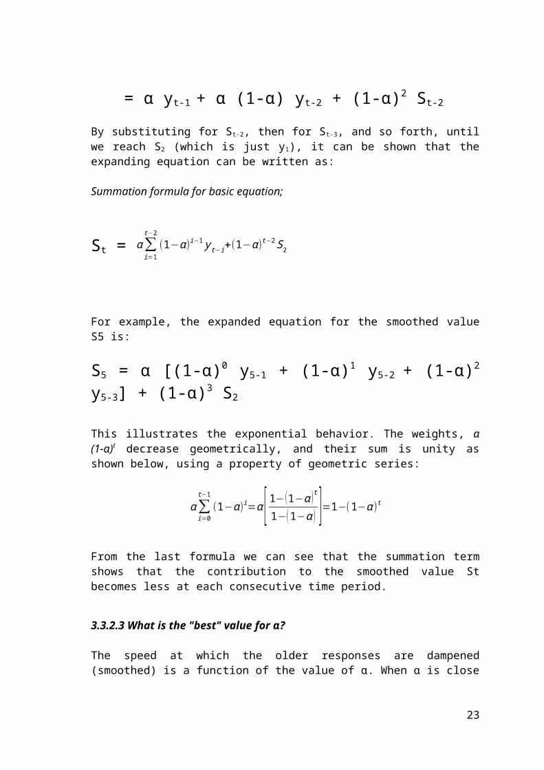
By substituting for St-2, then for St-3, and so forth, until we reach S2 (which is just y1), it can be shown that the expanding equation can be written as:

Summation formula for basic equation;

St = α∑i=1

t−2

(1−α )i−1 y t−i+(1−α)t−2 S2

For example, the expanded equation for the smoothed value S5 is:

S5 = α [(1-α)0 y5-1 + (1-α)1 y5-2 + (1-α)2 y5-3] + (1-α)3 S2

This illustrates the exponential behavior. The weights, α (1-α)t decrease geometrically, and their sum is unity as shown below, using a property of geometric series:

α∑i=0

t−1

(1−α )i=α [ 1−(1−α )t

1− (1−α ) ]=1−(1−α )t

From the last formula we can see that the summation term shows that the contribution to the smoothed value St becomes less at each consecutive time period.

3.3.2.3 What is the "best" value for ?α

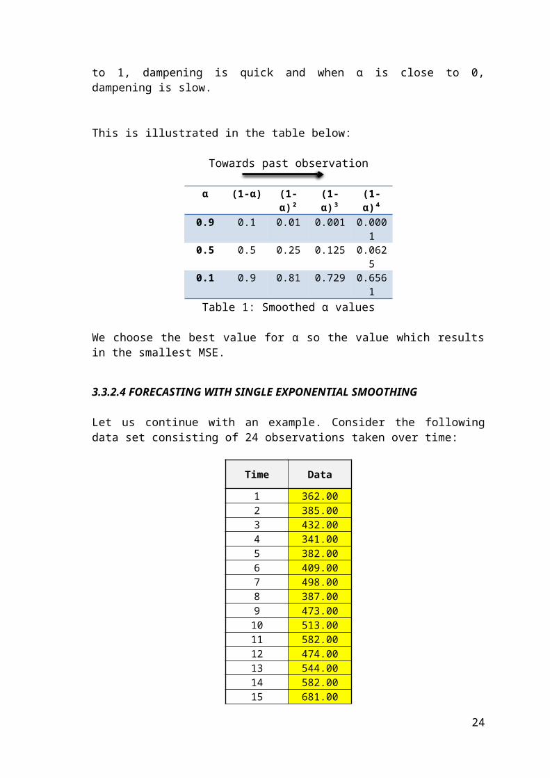
The speed at which the older responses are dampened (smoothed) is a function of the value of α. When α is close to 1, dampening is quick and when α is close to 0, dampening is slow.

This is illustrated in the table below:

Towards past observation

α (1-α) (1-α)² (1-α)³ (1-α)⁴

16

0.9 0.1 0.01 0.001 0.00010.5 0.5 0.25 0.125 0.06250.1 0.9 0.81 0.729 0.6561

Table 1: Smoothed α values

We choose the best value for α so the value which results in the smallest MSE.

3.3.2.4 FORECASTING WITH SINGLE EXPONENTIAL SMOOTHING

Let us continue with an example. Consider the following data set consisting of 24 observations taken over time:

Time Data

1 362.002 385.003 432.004 341.005 382.006 409.007 498.008 387.009 473.00

10 513.0011 582.0012 474.0013 544.0014 582.0015 681.0016 557.0017 628.0018 707.0019 773.0020 592.0021 627.0022 725.0023 854.0024 661.00

Table 2: Data Set for Single Exponential Smoothing ExampleForecasting Formula

The forecasting formula is the basic equation.St+1=α y t+(1−α ) S t 0 < α ≤ 1

t > 0This can be written as:

17

St+1=St +α (εt)

where ε tis the forecast error (actual - forecast) for period t.In other words, the new forecast is the old one plus an adjustment for the error that occurred in the last forecast.

α0.7

SIN

GLE

EXPO

NEN

TIAL

SM

OO

THIN

G

Timet

Datayt

ForecastSt+1

Error(yt – St+1)

Error Squared

1 362.002 385.00 362.00 23.00 529.003 432.00 378.10 53.90 2,905.214 341.00 415.83 -74.83 5,599.535 382.00 363.45 18.55 344.146 409.00 376.43 32.57 1,060.507 498.00 399.23 98.77 9,755.438 387.00 468.37 -81.37 6,620.939 473.00 411.41 61.59 3,793.2410 513.00 454.52 58.48 3,419.5311 582.00 495.46 86.54 7,489.7012 474.00 556.04 -82.04 6,730.0813 544.00 498.61 45.39 2,060.1514 582.00 530.38 51.62 2,664.2815 681.00 566.52 114.48 13,106.8116 557.00 646.65 -89.65 8,037.9317 628.00 583.90 44.10 1,945.1318 707.00 614.77 92.23 8,506.5719 773.00 679.33 93.67 8,773.9420 592.00 744.90 -152.90 23,378.1721 627.00 637.87 -10.87 118.1522 725.00 630.26 94.74 8,975.4923 854.00 696.58 157.42 24,781.6024 661.00 806.77 -145.77 21,249.91

Sum of Squared Errors (SSE) 171,845.44Mean of the Squared Errors (MSE) 7,471.54

Table 3: Forecasting ResultsIn the table above, the α value was determined as 0.7 by applying the MSE rule. The column filled with yellow shows the actual data and the blue one shows forecasting for related t time.

18

0 2 4 6 8 10 120.00

2.00

4.00

6.00

8.00

10.00

12.00

DATASingle

Graphic 1

Here is the graphical illustration of the actual data vs. forecast. As you can see in the graph, single exponential smoothing cannot cover the trend and seasonality in the given data. That’s why the forecast line always shows a lag just after the actual data.

Bootstrapping of Forecasts

What happens if you wish to forecast from some origin, usually the last data point, and no actual observations are available? In this situation we have to modify the formula to become:

St +1=α yorigin+ (1−α ) St

where yorigin remains constant. This technique is known as bootstrapping.

3.3.3 DOUBLE EXPONENTIAL SMOOTHING

Double exponential smoothing uses two constants and is better at handling trends

Single Smoothing does not excel in following the data when there is a trend. This situation can be improved by the introduction of a second equation with a

second constant, β, which must be chosen in conjunction with α.

19

Here are the two equations associated with Double Exponential Smoothing:

St = α yt + (1-α) (St-1 + bt-1) 0 ≤ α ≤ 1bt = β (St – St-1) + (1-β) bt-1 0 ≤ β ≤ 1

Note that the current value of the series is used to calculate its smoothed value replacement in double exponential smoothing.

Meaning of the smoothing equations

The first smoothing equation adjusts St directly for the trend of the previous period, b t-1,

by adding it to the last smoothed value, S t-1. This helps to eliminate the lag and brings S t

to the appropriate base of the current value.

The second smoothing equation then updates the trend, which is expressed as the difference between the last two values. The equation is similar to the basic form of single smoothing, but here applied to the updating of the trend.

3.3.3.1 Initial Values

Several methods to choose the initial values

As in the case for single smoothing, there are a variety of schemes to set initial values for St and bt in double smoothing. S1 is in general set to y1. Here are three suggestions for b1:

b1 = y2 - y1

b1 = [(y2 - y1) + (y3 - y2) + (y4 - y3)]/3b1 = (yn - y1) / (n - 1)

3.3.3.2 FORECASTING WITH DOUBLE EXPONENTIAL SMOOTHING

The one-period-ahead forecast is given by:

F t+ 1=S t+b t

The m-periods-ahead forecast is given by:

F t+m=St+mb t

Let us explain the double exponential smoothing with an example. Consider the following data set is given;

α β0.7 0.6

DOU

BLE

EXPO

NEN

TIAL

SM

OO

THIN

G

Time yt bt St Ft Error Error Squared

1 362.00 23.00 362.00 385.00 -23.00 529.002 385.00 23.00 385.00 408.00 -23.00 529.003 432.00 33.08 424.80 457.88 -25.88 669.774 341.00 -16.01 376.06 360.05 -19.05 363.075 382.00 -6.79 375.42 368.62 13.38 178.926 409.00 10.17 396.89 407.05 1.95 3.797 498.00 48.36 470.72 519.08 -21.08 444.338 387.00 -7.11 426.62 419.51 -32.51 1,057.159 473.00 15.35 456.95 472.31 0.69 0.4810 513.00 32.44 500.79 533.24 -20.24 409.5511 582.00 52.93 567.37 620.30 -38.30 1,466.6012 474.00 -8.52 517.89 509.37 -35.37 1,251.0013 544.00 6.03 533.61 539.64 4.36 19.0414 582.00 23.82 569.29 593.11 -11.11 123.4115 681.00 60.73 654.63 715.37 -34.37 1,180.9616 557.00 -5.78 604.51 598.73 -41.73 1,741.2717 628.00 6.51 619.22 625.73 2.27 5.1518 707.00 40.65 682.62 723.27 -16.27 264.5619 773.00 61.53 758.08 819.61 -46.61 2,172.8620 592.00 -34.06 660.28 626.22 -34.22 1,171.0621 627.00 -33.74 626.77 593.03 33.97 1,153.9622 725.00 21.69 685.41 707.10 17.90 320.4023 854.00 83.39 809.93 893.32 -39.32 1,546.0024 661.00 -14.18 730.70 716.51 -55.51 3,081.45

 Table 4 Sum of Squared Errors (SSE) 19,682.79Mean of the Squared Errors (MSE) 820.12

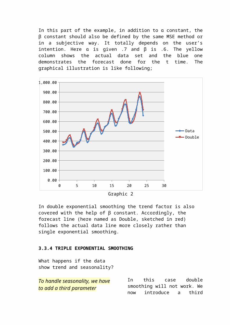
In this part of the example, in addition to α constant, the β constant should also be defined by the same MSE method or in a subjective way. It totally depends on the user’s intention. Here α is given .7 and β is .6. The yellow column shows the actual data set and the blue one demonstrates the forecast done for the t time. The graphical illustration is like following;

0 5 10 15 20 25 300.00

100.00

200.00

300.00

400.00

500.00

600.00

700.00

800.00

900.00

1,000.00

DataDouble

Graphic 2

In double exponential smoothing the trend factor is also covered with the help of β constant. Accordingly, the forecast line (here named as Double, sketched in red) follows the actual data line more closely rather than single exponential smoothing.

3.3.4 TRIPLE EXPONENTIAL SMOOTHING

What happens if the data show trend and seasonality?

To handle seasonality, we have to add a third parameter

In this case double smoothing will not work. We now introduce a third equation to take care of seasonality (sometimes called periodicity). The resulting set of equations is called the “Holt-Winters” (HW) method after the names of the inventors.

The basic equations for their method are given by:

bt = β (St – St-1) + (1 – β) bt-1 Trend Smoothing

It = γ y t

St+ (1−γ ) I t−L Seasonal Smoothing

St = α y t

I t−L+(1−α )(S t−1+bt−1) Overall Smoothing

Ft+m = (St + mbt) It-L+m Forecast

where y is the observation S is the smoothed observation b is the trend factor I is the seasonal index F is the forecast at m periods ahead t is an index denoting a time period 0 ≤ α ≤ 1, 0 ≤ β ≤ 1, 0 ≤ γ ≤ 1

and α, β, and γ are constants that must be estimated in such a way that the MSE of the error is minimized.

Complete season needed

To initialize the HW method we need at least one complete season’s data to determine initial estimates of the seasonal indices It-L.

L periods in a season

A complete season’s data consists of L periods. And we need to estimate the trend factor from one period to the next. To accomplish this, it is advisable to use two complete seasons; that is, 2L periods.

3.3.4.1 Initial values for the trend factor

How to get initial estimates for trend and seasonality parameters

The general formula to estimate the initial trend is given by

b = 1L ( y L+1− y1

L+

yL+2− y2

L+…+

yL+L− yL

L )

23

3.3.4.2 Initial values for the Seasonal Indices

Let us continue with an example. We work with data that consist of 6 years with 4 periods (that is, 4 quarters) per year. Then

Step 1: Compute the averages of each of the 6 years

Ap = ∑i=1

4

y i

4p= 1,2, ..., 6

Step 2: Divide the observations by the appropriate yearly mean

1 2 3 4 5 6

y1/A1 y5/A2 y9/A3 y13/A4 y17/A5 y21/A6

y2/A1 y6/A2 y10/A3 y14/A4 y18/A5 y22/A6

y3/A1 y7/A2 y11/A3 y15/A4 y19/A5 y23/A6

y4/A1 y8/A2 y12/A3 y16/A4 y20/A5 y24/A6

Step 3: Now the seasonal indices are formed by computing the average of each row. Thus the initial seasonal indices (symbolically) are:

I1 = ( y1/A1 + y5/A2 + y9/A3 + y13/A4 + y17/A5 + y21/A6)/6 I2 = ( y2/A1 + y6/A2 + y10/A3 + y14/A4 + y18/A5 + y22/A6)/6 I3 = ( y3/A1 + y7/A2 + y11/A3 + y15/A4 + y19/A5 + y22/A6)/6 I4 = ( y4/A1 + y8/A2 + y12/A3 + y16/A4 + y20/A5 + y24/A6)/6

We now know the algebra behind the computation of the initial estimates.

3.3.4.3 FORECASTING WITH TRIPLE EXPONENTIAL SMOOTHING

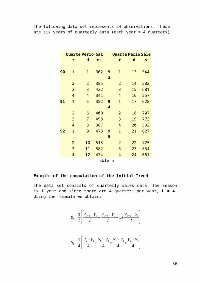
This example shows comparison of single, double and triple exponential smoothing for a data set.The following data set represents 24 observations. These are six years of quarterly data (each year = 4 quarters).

24

Quarter Period Sales Quarter Period Sales

90 1 1 362 93 1 13 5442 2 385 2 14 5823 3 432 3 15 6814 4 341 4 16 557

91 1 5 382 94 1 17 6282 6 409 2 18 7073 7 498 3 19 7734 8 387 4 20 592

92 1 9 473 95 1 21 6272 10 513 2 22 7253 11 582 3 23 8544 12 474 4 24 661

Table 5

Example of the computation of the Initial Trend

The data set consists of quarterly sales data. The season is 1 year and since there are 4 quarters per year, L = 4. Using the formula we obtain:

b1=1L [ y L+1− y1

L+

y L+2− y2

L+…+

y L+L− y L

L ]

b1=14 [ y5− y1

4+

y6− y2

4+

y7− y3

4+

y8− y4

4 ]

b1=14 [ 382−362

4+ 409−385

4+ 498−432

4+ 387−341

4 ]

b1=5+6+16.5+11.5

4=9.75

25

Example of the computation of the Initial Seasonal Indices

Step 1:

1 2 3 4 5 6

1 362 382 473 544 628 6272 385 409 513 582 707 7253 432 498 582 681 773 8544 341 387 474 557 592 661

Ap 380 419 510.5 591 675 716.75Table 6

In this example we used the full 6 years of data. Other schemes may use only 3, or some other number of years. There are also a number of ways to compute initial estimates.

Step 2:

1 2 3 4 5 6

362/380 382/419 473/510.5 544/591 628/675 627/716.75385/380 409/419 513/510.5 582/591 707/675 725/716.75432/380 498/419 582/510.5 681/591 773/675 854/716.75341/380 387/419 474/510.5 557/591 592/675 661/716.75

Table 7

Step 3:

I1 = (362/380 + 382/419 + 473/510.5 + 544/591 + 628/675 + 627/716.75) / 6 = 0.92

I2 = (385/380 + 409/419 + 513/510.5 + 582/591 + 707/675 + 725/716.75) / 6 = 1.01

I3 = (432/380 + 498/419 + 582/510.5 + 681/591 + 773/675 + 854/716.75) / 6 = 1.16

I4 = (341/380 + 387/419 + 474/510.5 + 557/591 + 592/675 + 661/716.75) / 6 = 0.92

26

α β γ0.6 0.7 0.7

TRIP

LE E

XPO

NEN

TIAL

SM

OO

THIN

G

Time yt St bt It Ft+m Error Error Squared

1 362.00 0.922 385.00 1.013 432.00 1.164 341.00 0.925 382.00 382.00 9.75 0.98 0.00 382.00 145,924.006 409.00 400.56 15.92 1.02 394.22 14.78 218.367 498.00 424.38 21.45 1.17 482.73 15.27 233.308 387.00 432.05 11.80 0.90 408.03 -21.03 442.329 473.00 468.37 28.97 1.00 433.12 39.88 1,590.5010 513.00 501.70 32.02 1.02 505.61 7.39 54.5711 582.00 512.17 16.93 1.15 623.99 -41.99 1,762.9812 474.00 527.09 15.53 0.90 477.02 -3.02 9.1313 544.00 543.55 16.18 1.00 542.43 1.57 2.4614 582.00 565.99 20.56 1.03 571.36 10.64 113.1715 681.00 591.11 23.75 1.15 672.30 8.70 75.6616 557.00 617.29 25.45 0.90 553.35 3.65 13.3217 628.00 633.72 19.14 0.99 643.04 -15.04 226.3418 707.00 674.58 34.34 1.04 669.85 37.15 1,380.4119 773.00 686.77 18.83 1.13 815.48 -42.48 1,804.9120 592.00 676.20 -1.75 0.88 636.18 -44.18 1,952.2921 627.00 648.32 -20.04 0.98 670.28 -43.28 1,873.3422 725.00 669.00 8.46 1.07 654.32 70.68 4,996.2123 854.00 723.24 40.51 1.17 767.56 86.44 7,472.4024 661.00 754.48 34.02 0.88 674.64 -13.64 186.08

 Table 8 Sum of Squared Errors (SSE) 170,331.73Mean of the Squared Errors (MSE) 8,516.59

Here in triple exponential smoothing besides the α and β constants, the user should also define γ constant in order to cover seasonality effect. The γ value is given as .7 in this example. Like in the previous example, the yellow column demonstrates the actual data and the blue column just shows the forecast done for the t period of time.

The most important notice for triple exponential smoothing is that there should be a complete observation of previous season in order to apply triple exponential smoothing, because the seasonality indices are the most important parts of the forecast. In this table, the first four red lines are just used to determine It seasonality indices.

0 5 10 15 20 25 300.00

100.00

200.00

300.00

400.00

500.00

600.00

700.00

800.00

900.00

DataTriple

Graphic 3

As you can see in the graphic sketched above, the triple exponential smoothing by covering both trend and seasonality effects, the both lines are nearly matched up with each other. They show the same ups and downs on the time horizon. This shows the power of the triple exponential smoothing.

0 5 10 15 20 25 300.00

100.00

200.00

300.00

400.00

500.00

600.00

700.00

800.00

900.00

1,000.00

DATASingle ExpoDouble ExpoTriple Expo

Graphic 4Overall graphic that shows all forecasts results with the different types of the smoothing.

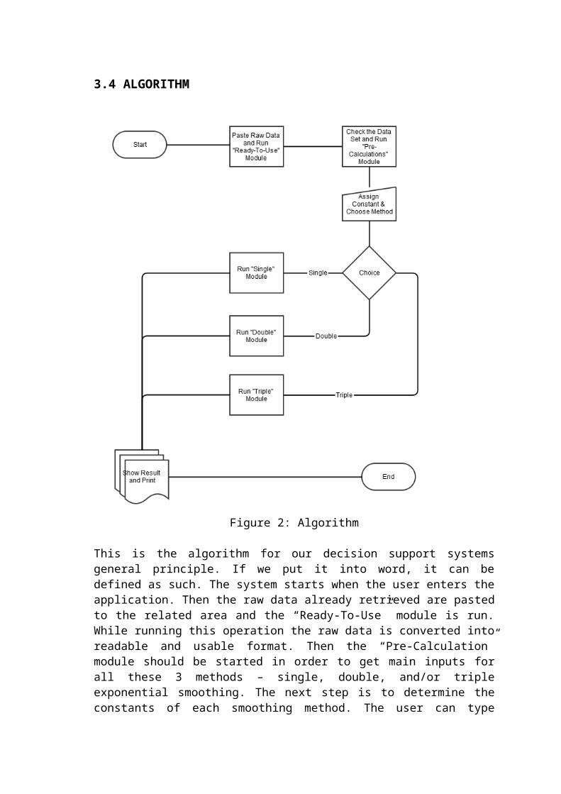
3.4 ALGORITHM

Figure 2: Algorithm

This is the algorithm for our decision support systems general principle. If we put it into word, it can be defined as such. The system starts when the user enters the application. Then the raw data already retrieved are pasted to the related area and the “Ready-To-Use” module is run. While running this operation the raw data is converted into readable and usable format. Then the “Pre-Calculation” module should be started in order to get main inputs for all these 3 methods – single, double, and/or triple exponential smoothing. The next step is to determine the constants of each smoothing method. The user can type manual input on this page and then decide to which method will be used. According to the user preference, the related module should be clicked in order to run preferred module. At the end of the each smoothing module, there will be a display page which shows entire report and graphical illustrations. As a final step, the user can take print outs, or export the report as a new Excel or PDF file format.

3.5 USER INTERFACES AND REPORTS

Instructions to Run Application

In order to run this application for the first time on the computer, steps below should be followed;

1. Once you open excel file, press ALT + F11 combination2. From macro window that shows up on the screen select Tools – References3. From Available Referenses window select Excel Solver.4. Save your changes first on the Makro screen and then save your excel file

Welcome Page

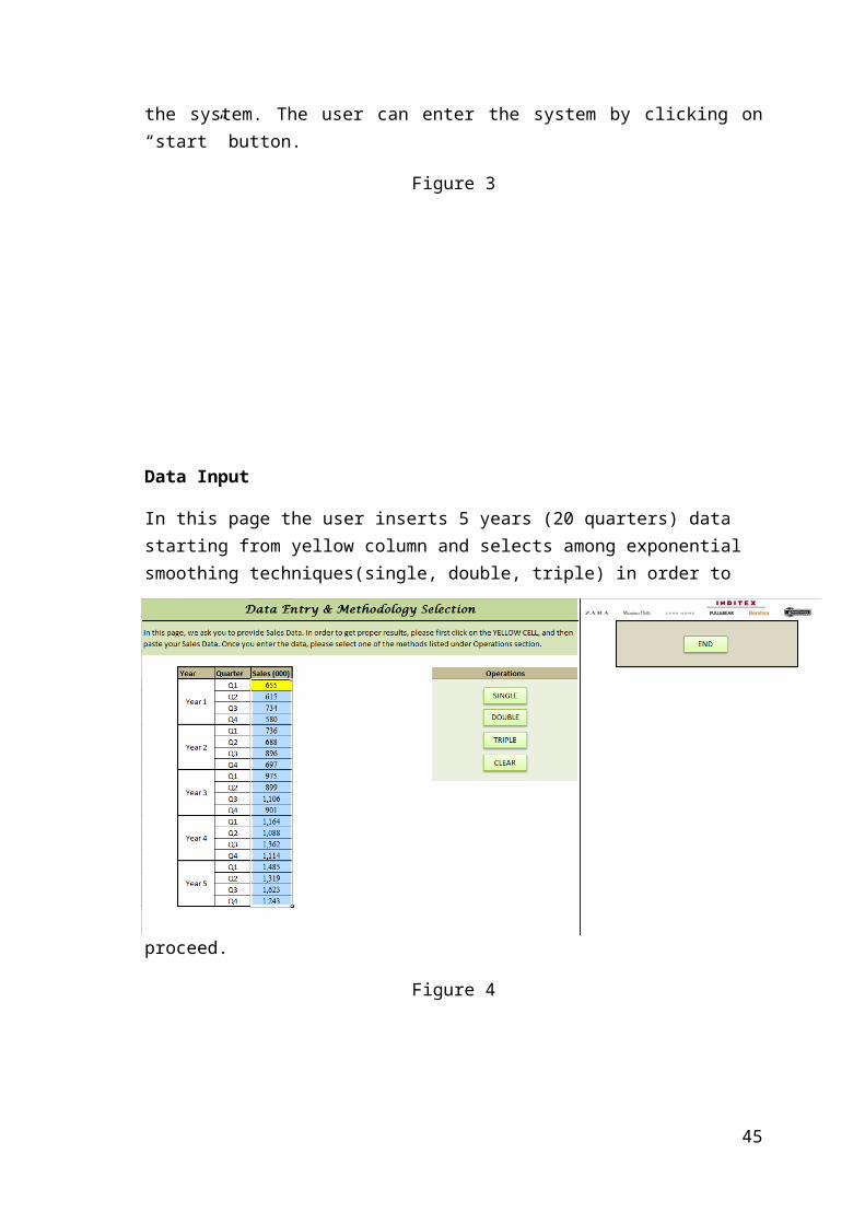
This is welcome page of the application. In this page there are certain types of instructions and general overview of the system. The user can enter the system by clicking on “start” button.

Figure 3

31

Data Input

In this page the user inserts 5 years (20 quarters) data starting from yellow column and selects among exponential smoothing techniques(single, double, triple) in order to proceed.

Figure 4

32

Single Exponential Smoothing Page

On this page the user can apply single exponential smoothing to the data entered on input page. There is an explanation under the title of the page where the user can learn about how to use the system and determine values to be selected. Once the user determines alpha value solve button should be clicked. After clicking on solve button forecast results will be displayed on the table and also graph for forecasting and growth rate will appear below the table. The user can see the graphs in a larger format by clicking on the graphs.

SEE CALC button used in order to see the calculation base on optimal Alfa value.

SAVE button is used for saving the results of the forecast as an excel sheet.

INPUT button allows the user to go back to input page so that the user can change the dataset or use a different method.

END button allows the user to leave the application.

SOLVE brings the results of the forecast for selected values

Question Marks could be selected in order to calculate MSE and MAD values to suggest the optimal values to be entered

Figure 5

33

This is the screen where the user can see the graph for forecasting in larger format. User can easily go back to single exponential smoothing page by clicking on BACK button or close the application by clicking on END.

Figure 6

This is the screen where the user can see the graph for expected cumulative growth rate for sales in a larger format. User can easily go back to exponential smoothing page by clicking on BACK button or close the application by clicking on END.

Figure 7

34

Double Exponential Smoothing Page

On this page the user can apply double exponential smoothing to the data entered on input page. There is an explanation under the title of the page where the user can learn about how to use the system and determine values to be selected. In addition to Alfa value the user needs to select another value called Beta which handles trend factor. After clicking on solve button forecast results will be displayed on the table and also graph for forecasting and growth rate will appear below the table. The user can see the graphs in a larger format by clicking on the graphs.

SEE CALC button used in order to see all calculations for entire Alfa and Beta values that could be selected.

SAVE button is used for saving the results of the forecast as an excel sheet.

INPUT button allows the user to go back to input page so that the user can change the dataset or use a different method.

END button allows the user to leave the application.

SOLVE brings the results of the forecast for selected values

Question Marks could be selected in order to calculate MSE and MAD values to suggest the optimal values to be entered

Figure 8

35

This is the screen where the user can see the graph for forecasting in larger format. User can easily go back to double exponential smoothing page by clicking on BACK button or close the application by clicking on END.

Figure 9

This is the screen where the user can see the graph for expected cumulative growth rate for sales in a larger format. User can easily go back to double exponential smoothing page by clicking on BACK button or close the application by clicking on END.

Figure 10

Triple Exponential Smoothing Page

On this page the user can apply triple exponential smoothing to the data entered on input page. There is an explanation under the title of the page where the user can learn about how to use the system and determine values to be selected. In addition to Alfa and beta values the user needs to select another value called Gamma which handles seasonality factor. After clicking on solve button forecast results will be displayed on the table and also graph for forecasting and growth rate will appear below the table. Once the solve button clicked, the user does not need to click on the solve button again in order to do forecasting with different Alfa, Beta and Gamma values since changing

36

Alfa, Beta and Gamma from spin buttons automatically updates the forecast for new values. The user can see the graphs in a larger format by clicking on the graphs.

SEE CALC button used in order to see all calculations for entire Alfa, Beta and Gamma values that could be selected.

SAVE button is used for saving the results of the forecast as an excel sheet.

INPUT button allows the user to go back to input page so that the user can change the dataset or use a different method.

END button allows the user to leave the application.

SOLVE brings the results of the forecast for selected values

Question Marks could be selected in order to calculate MSE and MAD values to suggest the optimal values to be entered

Figure 11

This is the screen where the user can see the graph for forecasting in larger format. User can easily go back to triple exponential smoothing page by clicking on BACK button or close the application by clicking on END.

37

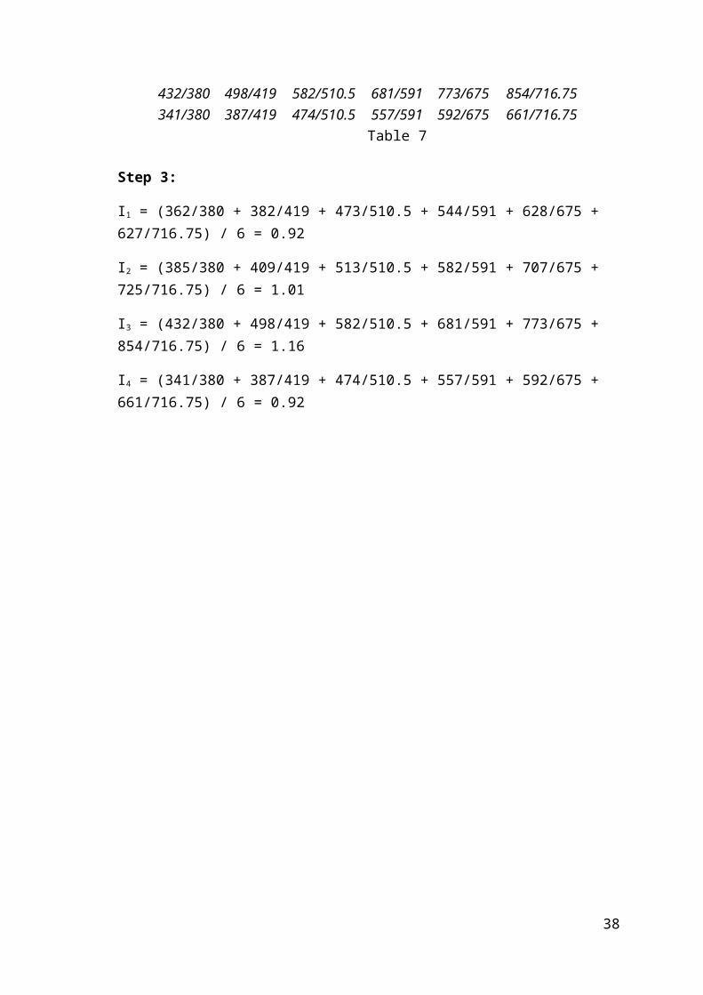
Figure 12

This is the screen where the user can see the graph for expected cumulative growth rate for sales in a larger format. User can easily go back to triple exponential smoothing page by clicking on BACK button or close the application by clicking on END.

Figure 13

Calculations Page

The user can see the calculations for optimal Alfa, Beta and Gamma values by clicking on “See Calc” button. The table below displayed only on triple exponential smoothing calculation page since it is only method that handles seasonality effect.

Figure 14

38

Table below can only be seen on single exponential smoothing calculation page and it shows the calculations for optimal Alfa value.

Figure 15

Table below can only be seen on double exponential smoothing calculation page and it shows the calculations for optimal Alfa and Beta values.

Figure 16

Table below can only be seen on triple exponential smoothing calculation page and it shows the calculations for optimal Alfa, Beta and Gamma values.

39

Figure 17

Message Boxes

1. Excel Solver

Once the user clicks on question marks, message box below appears. The user should select OK to proceed.

40

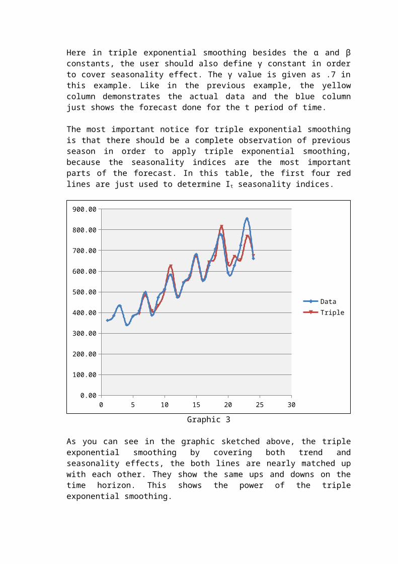
Figure 18

2. Invalid Data Entry for Alfa, Beta and Gamma Values

If the user enters any value which is not between 0 and 1 or any character, the error message below shows up.

Figure 19

4. ASSESSMENT

This work is a group work so we have a team that includes five persons. The team members are Philipp Jung, Uğur Keskin*, Recep Soner Kılıç, Nebile Kodaz, and Murat Usta. For this term project, we have a master plan. It covers almost three months so we

41

do have to have a master plan. At the beginning we envision the master plan and soon we update it as needed.

There are three main phase of the project; the project proposal, the mid report and presentation, lastly the final report and presentation. Except Uğur Keskin, all group members join the meetings actively.

The first phase of project is project proposal phase. The team is shaped on time. In the team, the project manager, Murat Usta organizes meetings and leads the other team members. In the first meetings, DSS are discussed and project proposal is determined. Additionally, DSS components, history and functions are studied. The team decides on project title: Sales Forecasting of INDITEX Corporation. Decision environment is bordered. The team goes over what can be the errors of the system. The scope of the project and mission of the project are noticed. Historical data are used for forecasting, and the results are sketched on graphs. The method of forecasting would be exponential smoothing. Also a presentation of project proposal is performed on the date that is assigned in the calendar of project by the instructor. In this phase the team designed its own work schedule on a master plan. Especially among the team members, Philipp, Soner and Murat have worked actively and presented the project proposal.

In the second phase a literature review was done. Exponential smoothing method is searched elaborately. The other forecasting methods are compared with the exponential method. The advantages and disadvantages of these forecasting methods are discussed. Some of our literature review materials are articles from science direct database and some books that are related with forecasting in business. Also one of the previous courses textbook has a chapter of forecasting. All the sources were distilled. Exponential smoothing types are explained clearly and elaborately in the mid report. We have defined the inputs and outputs of the DSS. The architecture of the DSS is figured out. The algorithm of the system is sketched. Also a prototype of the project is presented in this phase. Nebile, Soner and Murat have worked actively and presented the literature review of the project.

Lastly, in the final phase the project is implemented with real data. Excel macros and Solver are utilized in the project design. The interfaces are designed in a user friendly style. Some operational buttons and navigational buttons automate the macros. Some explanations and directions take place in interfaces. Alfa, Beta, and Gama forecast constants are able to be optimized by user. There is a table for the results of all three forecast methods; single, double and triple exponential smoothing. Also the graphs show the results illustratively. The success of forecast methods can be seen clearly in the graphs. Almost perfect match is obtained between forecasted values and real values. Lastly the presentation is performed and some improvements are suggested by the instructor. In this phase of project, Murat designs and implements the decision tool, Soner and Nebile test the work done by Murat and work on the report, Philipp has the responsibilities for the presentation.During the project processes, the team creates a decision support system in a harmonic group working style. The components of the DSS are included in the project: the data that comes from real databases of INDITEX, the method that is exponential smoothing method and lastly user interfaces and implementations that are realized in Excel. The team believes this project work is very successful, useful and efficient for the course’s coverage and learning activities.

42

5. PROJECT PLAN

The Sales Forecasting System has three documentation phases: proposal, mid-report, and final report. For each documentation phase, the project has several main tasks listed below:

MASTER PLANProject Code SFS001Project Title SALES FORECASTING

SYSTEMTeam Members Jung, Philipp

Keskin, UğurKılıç, Recep SonerKodaz, NebileUsta, Murat

Phase Planned ActualComplete%Start Finish Start Finish

Team Formation 04 Oct 05 Oct 04 Oct 05 Oct 100%

Project Proposal 11 Oct 23 Oct 13 Oct 23 Oct 100%

Presentation 21 Oct 23 Oct 22 Oct 23 Oct 100%Literature Review (Library, Web, former studies) 24 Oct 13 Nov 24 Oct 13 Nov 100%Interviews with experts, decision makers in the related area 24 Oct 13 Nov 24 Oct 13 Nov 100%

Development of the model 14 Nov 25 Nov 14 Nov 17 Nov 100%

Mid-report 24 Oct 25 Nov 20 Oct 25 Nov 100%

Presentation 25 Nov 27 Nov 27 Nov 100%

Data Collection and Organization 28 Nov 08 Dec 100%

Coding interfaces 09 Dec 22 Dec 100%

Validation (Optional) 09 Dec 23 Dec 100%

Final Report 28 Nov 23 Dec 28 Nov 23 Dec 100%

Presentation 23 Dec 23 Dec 23 Dec 100%Table 9

Coordinator: Murat Usta

Meetings:Meetings will be held at North Campus Study Hall at least once a week. Meeting time is 7 PM but it is subject to change group members’ availability during the planned day.

Task Allocation:

43

Each team member has the same responsibility level, but the coordinator of the team has more accountability. So, task allocation will be done by team coordinator fairly according to know-how and ability of team members.

6. CONCLUSION

The Sales Forecasting Decision Support System is created in the project. This system realizes its goal that is providing the sales forecasting report which is requested by supervisors or managers. According to that report the managers occasionally take actions regarding their department works. Sales forecasting system has all components of a DSS tool. Our inputs are obtained from sales database from the relevant department of INDITEX. The DSS tool uses the historical data and provides a suggestion for sales for the decision makers. The interfaces are designed as easy to understand and use. The outputs can be stored as Excel files.

The next step can be some applications of data mining techniques. The historical data that is obtained from sales can be trained as a times series in data mining. Some random variables make more difficult the design of different decision making tools. For example the market of the company is Euro Zone and some Middle East countries. International market has already had some hard conditions to compete. The variety of INDITEX market is a challenging case for modeling a decision support system tool. All countries have different economic and cultural characteristics. Also there are different risk factors such as the global crises in the market. In this domain, working on a time series is already too complex as well as the differentiations of INDITEX market. After design a system for INDITEX, the customization of the system is a need for each zone. In conclusion, in the INDITEX case DSS tools or Data Mining tools requires big efforts to design and implement.

7. REFERENCES

1. BHARGAVA, Hemant K.; POWER, Daniel J.; SUN, Daewon (2005) “Progress in Web-based decision support technologies” pp.1083-1095.

2. BURSTEIN, Frada and  HOLSAPPLE ,Clyde W. (2008) “Handbook on Decision Support Systems 1” Springer.

3. CORBERÁN-VALLET, Ana; BERMÚDEZ, José, D.; VERCHER, Enriqueta (2011) “Forecasting Correlated Time Series With Exponential Smoothing Models”, International Journal of Forecasting 27 (2011) 252-265.

4. DE GOOIJER, Jan G. and HYNDMAN, Rob J. (2006) “25 Years of Time Series Forecasting”, International Journal of Forecasting 22 (2006) 443-473.

5. FICK, Göran; SPRAGUE, Ralph H.; Editors, Jr. (1980) “Decision Support Systems: Issues and Challenges” International Institute for Applied System Analysis.

6. HANKE, John E.; WICHERN, Dean W.; REITSCH, Arthur G. (2001) Business Forecasting, Prentice Hall.

7. KUO, R.J. and XUE, K.C. (1998) “An Intelligent Sales Forecasting System Through Integration of Artificial Neural Network and Fuzzy Neural Network”, Computers In Industry 37 (1998) 1-15.

44

8. MAKRIDAKIS, Spyros G. (1978) Forecasting : Methods and Applications, Wiley.

9. MORTON, M.S. Scott (1971) Management Decision Systems: Computer Based Support for Decision Making. Cambridge, Massachusetts: Harvard University, Division of Research.

10. NIST/SEMATECH e-Handbook of Statistical Methods, http://www.itl.nist.gov/div898/handbook/, 2013.

11. POWER, Daniel J.; KAPARTHI, Shashidhar (2002) “Building Web Based Decision Support Systems, Vol.11, No.4, pp. 291-292.

12. RENDER, Barry; STAIR, Ralph M.; HANNA, Michael E. (2009) Quantitative Analysis for Management, Pearson Prentice Hall.

13. SHIM, J.P.; WARKENTIN, Merrill; COURTNEY, James F.; POWER, Daniel J.; SHARDA, Ramesh; CARLSSON, Christer. (2002) “Past, present, and future of decision support technology” pp.111-126.

14. STEPNICKA, Martin; CORTEZ, Paulo; DONATE, Juan Peralta; STEPNICKA, Lenka (2013) “Forecasting Seasonal Time Series with Computational Intelligence: On Recent Methods and the Potential of Their Combinations”, Expert Systems with Applications 40 (2013) 1981-1992.

15. TASHMAN, Leonard J. and KRUK, Joshua M. (1996) “The Use of Protocols to Select Exponential Smoothing Procedures: A Reconsideration of Forecasting Competitions”, International Journal of Forecasting 12 (1996) 235-253.

45