1

Are Two Heads Better Than One?: Monetary Policy by Committee

by

Alan S. Blinder and John Morgan* Princeton University University of California, Berkeley

1. Introduction and Motivation

The old saw “it works in practice, now let’s see if it works in theory” has a direct

application to the design of monetary policy institutions. In recent years, central banking practice

has exhibited a notable shift from individual to group decisionmaking, that is, toward more

monetary policy committees (MPCs). For example, J.P. Morgan’s “Guide to Central Bank

Watching” (March 2000, p. 4) noted that “One of the most notable developments of the past few

years has been the shift of monetary policy decision-making to meetings of central bank policy

boards.” Two of the best-known examples of this institutional change are the Bank of England

and the Bank of Japan, which (roughly) switched from individual to group decisionmaking in

1997 and 1999 respectively. The Governing Council of the European System of Central Banks,

patterned loosely on the Federal Open Market Committee, also opened for business in 1999,

although the Bundesbank Council had made decisions as a group long before that.

Nevertheless, economic theory has had precious little to say on the pros and cons of

making monetary policy individually or in groups.1 Nor is there substantial empirical evidence

on the relative merits of the two types of monetary policy decisionmaking processes.

* Correspondence to John Morgan: morgan@haas.berkeley.edu. We gratefully acknowledge financial support from Princeton’s Center for Economic Policy Studies and thank Felix Vardy for excellent and extensive research assistance. 1 See, among other sources, Goodfriend (2000), Kristen (2001), and Gersbach and Hahn (2001) for recent discussions of the pros and cons of group versus committee decisionmaking on monetary policy. Blinder (forthcoming, 2003) contains a reasonably comprehensive survey of the (limited) literature on the question.

2

In fact, this chasm between theory and practice generalizes. While economics has been

characterized as the science of choice, almost all the choices economists analyze are modeled as

individual decisions. A consumer with a utility function and a budget constraint decides what to

purchase. A firm, modeled as an individual decisionmaker, decides what will maximize its

profits. A unitary central banker with a well-defined loss function selects the optimal interest

rate. In many instances, these modeling choices abstract away from the fact that a group is in fact

making the decision, presumably on the grounds that the group members have the same objective

and share the same information. The question, “Do decisions made by groups differ

systematically from the decisions of the individuals who comprise them?” is infrequently asked.2

But we all know that many decisions in real societies—including some quite important

ones—are made by groups. Legislatures, of course, make the laws. The Supreme Court is a

committee, as are all juries. Some business decisions, e.g., in partnerships or management

committees, are made collectively, rather than dictatorially. And, as just noted, monetary policy

in most countries these days is made by a committee rather than by an individual. While one of

us served as Vice Chairman of the Federal Reserve Board, he came to believe that economic

models might be missing something important by treating monetary policy decisions as if they

were made by a single individual maximizing a well-defined loss function. As Blinder (1998, p.

20) subsequently wrote:

While serving on the FOMC, I was vividly reminded of a few things all of us probably know about committees: that they laboriously aggregate individual preferences; that they need to be led; that they tend to adopt compromise positions on difficult questions; and—perhaps because of all of the above—that they tend to be inertial.

This sentiment reflects what is probably a widely-held view: that groups make decisions more

slowly than individuals. (In the case of monetary policy, slowness is reflected in the amount of

2 The most prominent and famous exception is surely Arrow (1963).

3

data the Fed feels compelled to accumulate before coming to a decision rather than in the length

of time a meeting takes.) One of the major questions for this paper is: Is it true?

But there is a deeper question: Why are so many important decisions entrusted to groups?

Presumably because of some belief in collective wisdom. In a complicated world, where no one

knows the true model or even all the facts, where data may be hard to process or to interpret, and

where value judgments may influence decisions, it may be beneficial to bring more than one

mind to bear on a question. While it has been said that nothing good was ever written by a

committee,3 could it be that committees actually make better decisions than individuals?

So these are the two central questions for this paper: Do groups such as monetary policy

committees reach decisions more slowly than individuals do? (We have never heard it suggested

that groups decide faster.) And are group decisions, on average, better or worse than individual

decisions?

Since neither the theoretical nor the empirical literature offers much guidance on these

questions, our approach is experimental. We created two laboratory experiments in which

literally everything was held equal except the nature of the decisionmaking body—an individual

or a group. Even the identities of the individuals were the same, since each experimental group

consisted of five people who also participated as individuals. We therefore had automatic,

laboratory controls for what are normally called "individual effects." The experimental setting

also allowed us to define an objective function—which was known to the subjects—that

distinguished better decisions from worse ones with a clarity that is rarely attainable in the real

world. That is one huge advantage of the laboratory approach. The artificiality is, of course, its

principal drawback.

3 The Bible is often offered as an exception.

4

The two experiments, which are described in detail below, were very different.4 In the

simpler setup, described in Section 3, we created a purely statistical problem devoid of any

economic content, but designed (as will be explained) to mimic certain aspects of monetary

policymaking: Subjects were asked to guess the composition of an (electronic) urn "filled" with

blue balls and red balls. In the more complex setup, discussed in Section 2, we placed subjects

explicitly in the shoes of monetary policymakers: Subjects were asked to steer an (electronic

model of an) economy by manipulating the interest rate.

The results were strikingly consistent across experimental designs. Neither experiment

supported the commonly-held belief that groups are more inertial than individuals. In fact, the

groups required no more data than the individuals before coming to a decision. That came as a

big surprise to us; our priors were like seemingly everyone else's. Despite the fact that both

groups and individuals were operating with similar amounts of information, both experiments

found that groups, on average, made better decisions than individuals. (Here our priors were

much more diffuse.) Moreover, groups outperformed individuals by almost exactly the same

margins in the two experiments.

In addition, the experiments unearthed one other surprising result: There were practically

no differences between group decisions made by majority rule and group decisions made under a

unanimity requirement. This finding, which also conflicted with our priors, is also highly

relevant to monetary policy. The ESCB, for example, reaches decisions unanimously while, e.g.,

the Bank of England relies on majority vote. (The Fed is somewhere in between, but probably

loser to the unanimity principle.)

Before proceeding, a few words on the experimental literature on individual versus group

choices may be useful. Much of it comes from psychology and centers on how individual biases

4 The data and program code for both experiments are available on request.

5

are reflected in group decisions. The evidence on whether groups or individuals make “better”

decisions in this framework is mixed. In a metastudy of this literature, Kerr et al. (1996)

concluded that there is no general answer to the question. Other studies have found that group

decisions can lead to excessive risk taking—the so-called risky shift, which we will discuss

later.5

In the economics literature, most individual-versus-group experiments are in game-

theoretic settings, rather than the decision-theoretic settings of our experiments. Some examples

are Bornstein and Yaniv (1998), Cox and Hayne (1998), and Kocher and Sutter (2000).

Methodologically, our paper is closest to Cason and Mui (1997), who explored individual and

group decisions with objective payoffs in a decision-theoretic setting. Their substantive

concerns, however, were completely different from ours. In particular, the decisionmaking task

in their experiment was quite straightforward, but there were potentially strong differences of

opinion about the allocation of rewards. Our experiments were structured in just the opposite

way: The decisionmaking task was complex, but there was no room for dispute over the division

of the spoils. Thus, our focus was mainly on differences between groups and individuals in what

psychologists refer to as intellective tasks rather than judgmental tasks.

The remainder of the paper is organized into four sections. Section 2 describes the

monetary policy experiment and what we found. Section 3 does the same for the urn experiment.

Section 4 reports briefly on some mainly-unsuccessful attempts to model the group

decisionmaking process, and Section 5 is a brief summary.

5 See, for example, Wallach, Kogan, and Bem (1964).

6

2. The Monetary Policy Experiment

Our main experiment asked subjects to assume the role of monetary policymaker. For this

reason, we imposed a prerequisite in recruiting subjects that we did not impose in the urn

experiment: They had to have taken at least one course in macroeconomics.

2.1 Description of the Monetary Policy Experiment

We brought students into the laboratory in groups of five, telling them that they would be

playing a monetary policy game. Specifically, we programmed each computer with a simple

two-equation macroeconomic model that approximates a canonical model made popular in the

recent theoretical literature on monetary policy,6 choosing (not estimating) parameter values that

resembled the U.S. economy:

(1) Ut − 5 = 0.6(Ut-1 − 5) + 0.3(it-1 − πt-1 − 5) - Gt + et

(2) πt = 0.4πt-1 + 0.3πt-2 + 0.2πt-3 + 0.1πt-4 − 0.5(Ut-1 − 5) + wt .

Equation (1) can be thought of as a reduced form combining an IS curve with Okun's

Law. Specifically, U is the unemployment rate, and the assumed "natural rate" is 5%. Since i is

the nominal interest rate and π is the rate of inflation, the term it − πt − 5 connotes the deviation

of the real interest rate from its equilibrium or "neutral" value, which is also set at 5%.7 Higher

(lower) real interest rates will push unemployment up (down), but only gradually. But our

experimental subjects, like the Federal Reserve, controlled only the nominal interest rate, not the

real interest rate.

The Gt term connotes the affect of fiscal actions on unemployment and is the random

event that our experimental monetary policymakers are supposed to recognize and react to. G

6 See, for example, Ball (1997) and Rudebusch and Svensson (1999). 7 The neutral real interest rate is defined as the real rate at which inflation is neither rising nor falling. See Blinder (1998, pages 31-33).

7

starts at zero and randomly changes to either +0.3 or −0.3 sometime within the first 10 periods.

As is clear from equation (1), this event changes unemployment by precisely that amount, but in

the opposite direction. Prior to the shock, the model's steady-state equilibrium is U = 5, i − π = 5.

Because the long-run Phillips curve is vertical, any constant inflation rate can be a steady state.

But we always began the experiment with inflation at 2%—which is the target rate. The shock

changes the "neutral" real interest rate to either 6% or 4%, as is apparent from the coefficients in

equation (1). Our subjects were supposed to react to this event, presumably with a lag, by raising

or lowering the nominal interest rate. The length of the lag, of course, is one of our primary

interests.

Equation (2) is a standard accelerationist Phillips curve. Inflation depends on the lagged

unemployment rate and on its own four lagged values, with weights summing to one. While the

weighted average of past inflation rates can be thought of as representing expected inflation, the

model does not demand this interpretation. The coefficient on the unemployment rate was chosen

to (roughly) match empirically-estimated Phillips curves for the United States.

Finally, the two stochastic shocks, et and wt, were drawn from uniform distributions on

the interval [−.25, +.25].8 Their standard deviations are approximately 0.14, or about half the size

of the G shock. This parameter controls the "signal to noise" ratio in the experiment. We tried to

size the fiscal shock to make it easy to detect, but not “too easy.”9

Monetary policy affects inflation only indirectly in this model, and with a distributed lag

that begins two periods later. All of our subjects understood that higher interest rates reduce

8 The distributions were uniform, rather than normal, for programming convenience. 9 This is a probabilistic statement. It is possible, for example, that a two-standard-deviation e or w shock in the opposite direction completely obscures the G shock.

8

inflation and raise unemployment with a lag, and that lower interest rates do the reverse.10 But

they did not know any details of the model's specification, coefficients, or lag structure. Nor did

they know when the shock occurred. But they did know the probability law that governed the

shock--which was a uniform distribution across periods 1 through 10.

While the model looks trivial, stabilizing such a system can be rather tricky in practice.

Because equation (2) builds in a unit root, the model will diverge from equilibrium when

perturbed by a G shock—unless it is stabilized by monetary policy. But the lags make the

divergence pretty gradual. One useful way to think about this dynamic instability is as follows.

Start the system at equilibrium with U = 5, π = 2, and i = 7, as we did. Now suppose G rises to

0.3. By (1), the neutral real rate of interest increases to 6%. So the initial real rate, which is 5%,

is now below neutral—and hence expansionary. With a lag, inflation begins to rise. If the central

bank fails to raise the nominal interest rate, the real rate falls further—stimulating the economy

even more.

Each play of the game proceeded as follows. We started the system in steady state

equilibrium with Gt=0, current and lagged nominal interest rates at 7% (reflecting a 5% real rate

and a 2% inflation target), lagged U at 5%, and all lags of π at 2%. The computer selected values

for the two random shocks and displayed the first-period values, U1 and π1, on the screen for the

subjects to see. Normally, these numbers were quite close to the optimal values of U = 5% and π

= 2%. In each subsequent period, new random values of et and wt were drawn, thereby creating

statistical noise, and the lagged variables that appear in equations (1) and (2) were updated. The

10 Remember, all of our subjects had at least some exposure to basic macroeconomics. Lest they had forgotten, the instructions (exhibited in the appendix) reminded them that raising the rate of interest would lower inflation and raise unemployment, while lowering the rate of interest would have the opposite effects.

9

computer would calculate Ut and πt and display them on the screen, along with all past values.

Subjects were then asked to choose an interest rate for the next period, and the game continued.

At some period chosen at random from a uniform distribution between t=1 and t=10, Gt

was either raised to +0.3 or lowered to −0.3. (Whether G rose or fell was also decided randomly.)

Students were not told when G changed, nor in which direction. Even though our primary

interest was in the decision lag, that is, the lag between the change in G and the change in the

interest rate, we did not stop the game when the interest rate was first changed because this

seemed unnatural in the monetary-policy context. Instead, each play of the game continued for

20 periods. (Subjects were told to think of each period as a quarter.)

It is important to note that no time pressure was applied; subjects were permitted to take

as much clock time as they pleased to make each decision. In comparing the speed with which

decisions are taken by individuals and groups, clock time is not what we are concerned with.

Some readers of earlier drafts were confused on this point, so let us be explicit. There are

certainly examples of real world decisions in which speed, in the literal sense of clock time, is of

the essence—think of skiing down a narrow slope, shooting the rapids, or auto racing. But very

few economic decisions are of this character. (Bond and commodity trading may be an

exception.) No one much cares if a consumer takes five minutes or five hours to decide on her

consumption bundle, nor if a firm takes an hour or a day to decide how much labor to hire.

Certainly in the context of monetary policy, clock time is irrelevant. Nobody cares

whether the FOMC, when it meets, deliberates for two hours or four hours. What is relevant, and

what is measured here as the decision lag, is the amount of data that the decisionmakers insist on

seeing before they change interest rates. In the real world, this data flow corresponds, albeit

unevenly, to calendar time—e.g., the Fed may see five relevant pieces of data one week, three

10

the next, etc. At some point, it decides that it has accumulated enough information to warrant

changing interest rates. In our experiment, data on unemployment and inflation flow evenly:

Each experimental period brings one new observation on each variable. So when we say that one

type of decisionmaking process “takes longer” than another, we mean that more data (not more

minutes) are required before the decision is made.

To evaluate the quality of the decisions, our other main interest, we need a loss function.

While quadratic loss functions are the rule in the academic literature, they are rather too difficult

for subjects to calculate in their heads. So we used an absolute-value function instead.

Specifically, subjects were told that their score for each quarter would be:

(3) st = 100 − 10Ut − 5 − 10πt − 2,

and the score for the entire game (henceforth, S) would be the (unweighted) average of st over

the 20 quarters. The coefficients in (3) scale the scores into percentages—giving them a ready,

intuitive interpretation. Equal weights on unemployment deviations and inflation deviations were

chosen to facilitate mental calculations: Every miss of 0.1 cost one point. Thus, for example,

missing the unemployment target by 0.5 (in either direction) and the inflation target by 0.7 would

result in a score of 100 − 12 = 88 for that period. At the end of the entire session, scores were

converted into money at the rate of 25 cents for each percentage point. Subjects typically earned

about $21-$22 out of a theoretical maximum of $25.

Finally, we "charged" subjects a fixed cost of 10 points each time they changed the rate

of interest, regardless of the size of the change.11 The reason is as follows. The random shocks, et

and wt, were an essential part of the experimental design because, without them, changes in Gt

would be trivial to observe: No variable would ever change until G did. After some

experimentation, we decided that random shocks with standard deviations about half the size of

11

the G shock made it neither too easy nor too difficult to discern the Gt "news" amidst the et and

wt "noise."

But this decision created an inference problem: Our subjects might receive several false

signals before G actually changed. For example, a two-standard-deviation e shock appears just

like a negative G shock, except that the latter is permanent while the former is transitory. (The

random shocks were iid.) Furthermore, subjects knew neither the size of the G shock nor the

standard deviations of e and w; so they had no way of knowing that a two-standard-deviation

disturbance would look (at first) like a G shock.

In some early trials designed to test the experimental apparatus, we observed students

moving the interest rate up and down frequently—sometimes every period. Such behavior would

make it virtually impossible to measure (or even to define) the decision lag in monetary policy.

So we instituted a small, 10-point charge for each interest rate change. Ten points is not much of

a penalty; averaged over a 20-period game, it amounts to just 0.5% of total score. But we found

it was large enough to deter most of the excessive fiddling with interest rates. It also had the

collateral benefit of making behavior much more realistic.12 The Fed does not jigger the interest

rate around every quarter, presumably because it perceives some cost of doing so that is not

captured in equation (3).13

The game was played as follows. Each session had five subjects, mostly Princeton

undergraduates. Subjects were read detailed instructions (shown in the appendix), which they

also had in front of them in writing, and then allowed to practice with the computer apparatus for

11 To keep things simple, only integer interest rates were allowed. 12 With one exception: Since the game terminated after 20 periods, students generally concluded that it was not worth paying 10 points to change the rate of interest in one of the last few periods. We pay virtually no attention to this end-game data. 13 Empirically estimated reaction functions for central banks typically include a ∆i term that is rationalized by some sort of cost of changing interest rates.

12

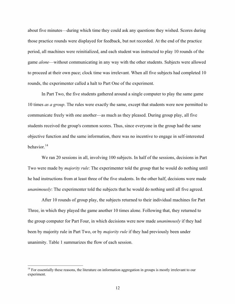
about five minutes—during which time they could ask any questions they wished. Scores during

those practice rounds were displayed for feedback, but not recorded. At the end of the practice

period, all machines were reinitialized, and each student was instructed to play 10 rounds of the

game alone—without communicating in any way with the other students. Subjects were allowed

to proceed at their own pace; clock time was irrelevant. When all five subjects had completed 10

rounds, the experimenter called a halt to Part One of the experiment.

In Part Two, the five students gathered around a single computer to play the same game

10 times as a group. The rules were exactly the same, except that students were now permitted to

communicate freely with one another—as much as they pleased. During group play, all five

students received the group's common scores. Thus, since everyone in the group had the same

objective function and the same information, there was no incentive to engage in self-interested

behavior.14

We ran 20 sessions in all, involving 100 subjects. In half of the sessions, decisions in Part

Two were made by majority rule: The experimenter told the group that he would do nothing until

he had instructions from at least three of the five students. In the other half, decisions were made

unanimously: The experimenter told the subjects that he would do nothing until all five agreed.

After 10 rounds of group play, the subjects returned to their individual machines for Part

Three, in which they played the game another 10 times alone. Following that, they returned to

the group computer for Part Four, in which decisions were now made unanimously if they had

been by majority rule in Part Two, or by majority rule if they had previously been under

unanimity. Table 1 summarizes the flow of each session.

14 For essentially these reasons, the literature on information aggregation in groups is mostly irrelevant to our experiment.

13

Table 1 The Flow of the Monetary Policy Experiment

Instructions Practice Rounds (no scores recorded) Part One: 10 rounds played as individuals Part Two: 10 rounds played as a group under majority rule (alternatively, under unanimity) Part Three: 10 rounds played as individuals Part Four: 10 rounds played as a group under unanimity (alternatively, under majority rule) Students are paid in cash, fill out a short questionnaire, and leave.

A typical session (of 40 plays of the game) lasted about 90 minutes. Each of the 20

sessions generated 20 individual observations per subject, or 2,000 in all, and 20 group

observations, or 400 in all. We would have liked to have taken longer and generated more

observations, but it was unrealistic to ask subjects to commit more than two hours of their time,15

and 40 plays of the game were about all we could count on finishing within that time frame.

2.2 The Three Main Hypotheses

While several subsidiary questions will be considered below, our interest focused on the

three main hypotheses mentioned in the introduction, especially the first two:

H1: Group decisions are more inertial than individual decisions.

The main idea that motivated this study was our prior belief that groups are inertial---that

is, they need to accumulate more data before coming to a decision. We repeat once again that we

measure the decision lag in number of periods—that is, the amount of information required

before a decision is reached—not in elapsed clock time, which, in the context of monetary

15 Although sessions normally took closer to 1 1/2 hours, we insisted that subjects agree to commit two hours, since the premature departure of even one subject would ruin an entire session.

14

policy, seemed irrelevant and was not measured.16 The decision lag, L, can be positive, as was

true in 84.8% of the cases, or negative (if subjects change the interest rate before G changes).

Specifically, let Li be the average lag for the i-th individual in the group (i = 1,…, 5)

when he or she plays the game alone, and let LG be the average lag for those same five people

when making decisions as a group. Under the null hypothesis of no group interaction, the

group's mean lag would equal the average of the five individual mean lags:

LG = (L1 + L2 + L3 + L4 + L5)/5.

Furthermore, under this null, and assuming independence across observations, a simple t-test for

difference in means is the appropriate test.17

The typical lags in the monetary policy game were actually quite short, averaging just

over 2.4 "quarters" across the 2400 observations. In fact, a number of subjects "jumped the gun"

by moving interest rates before G had changed. (As just noted, this happened in 15.2% of all

cases.) Surprisingly, the groups actually made decisions slightly faster than the individuals on

average, with a mean lag of just 2.30 periods (with standard deviation 2.75) versus 2.45 periods

(with standard deviation 3.50) for the individual decisions. While this scant 0.15 difference goes

in the direction opposite to the null hypothesis, it does not come close to statistical significance

at conventional levels (t = 0.78, p = .22 in a one-tailed test). Histograms for the variable L for

individuals and groups look strikingly alike. (See Figure 1.) In fact, the left-hand panel resembles

a mean-preserving spread of the right-hand panel. In a word, we find no experimental support for

the commonsense belief that groups are more inertial than individuals in their decision making.

16 It was clear from observing the experiments, however, that groups took more clock time. 17 We thank Alan Krueger for reminding us of this simple consequence of the Neymann-Pearson lemma.

15

Individual Play Group Play

Fra

ctio

n

Lag-10 0 10 20

0

.1

.2

.3

.4

Fra

ctio

n

Lag-10 0 10 20

0

.1

.2

.3

.4

Figure 1: Histograms of Lag in Monetary Experiment

Before examining this counterintuitive finding further, an important methodological issue

must be addressed. The t-test that we just employed treats each play of the game as an

independent observation. But in presenting this work to several audiences, we found some

people insisting that strong individual effects (e.g., person i is inherently slower than person j)

meant that the 40 observations on the behavior of one person in a single session were far from

independent. In Section 4, we will present clear evidence that individual effects were actually

quite unimportant in our experiments. But in order to establish that our findings do not rest on

the independence assumption, we will also present tests based on an extremely conservative view

of the data that treats each session as a single observation. Doing that collapses our 2400

observations into just 20 matched pairs of individual and group lags and, when treating the data

this way, we use the Wilcoxon signed-ranks test. In this particular application, the Wilcoxon test

16

detects no significant difference between the groups and the individuals (z=0.5 in a one-tailed

test).18

The more important question is: Could the counterintuitive finding of (statistically) equal lags

be an artifact of the experiment? One possibility relates to learning.19 In both of our experiments,

subjects always began by making decisions as individuals. Suppose the typical student was still

learning how to play the game in these early rounds of individual play—even though he or she

had been given the opportunity to practice before the start of the game. In that case, learning

effects could mask the fact that individuals are “really” faster than groups once they have learned

how to play the game—thus biasing our results toward showing no significant differences in

average lags between individuals and groups.

We examined this possibility as follows. Discarding the data from Part One (rounds 1-

10), we compared individual decisions in Part Three (rounds 21-30) with group decisions made

just before (in Part Two, rounds 11-20) and just after (in Part Four, rounds 31-40) . Interestingly,

in 12 of the 20 sessions, the average of the individual lags in Part Three actually exceeded the

average of the group lags in Part Two. This difference is significant at conventional levels

regardless of whether we treat an individual decision as the unit of observation (t = 2.0) or the

session as the unit of observation (z = 1.9). Comparing individual lags in Part Three with group

lags in Part Four, however, shows no significant difference (t = 1.6, z = 0.6). To summarize,

there is no evidence to support the notion that learning accounts for our finding that group and

individual lags are similar.

Another possible explanation for why we might be seeing no differences between

individual and group lags is the phenomenon labeled the “risky shift” in the psychology

18 Of course, no test will have much power with only 20 observations. The Wilcoxon test results are more interesting when we try to demonstrate differences rather than deny them, as we do just below.

17

literature. The risky shift is the observation that the diffusion of responsibility in groups leads

them to take on more risk than they would as individuals. In our setting, one way in which

groups could implement a riskier strategy would be to make decisions sooner (that is based on

less information)--and this effect just might compensate for the group inertia that we expect to

see (but do not find).

Fortunately, there is second way in which groups could take more risk in the monetary

policy experiment: by making larger interest rate changes when they decide to move. Thus, if

the risky shift is empirically important in our experiment, we should find that the average size of

the initial interest rate change is larger for groups than for individuals. This hypothesis is directly

testable with our data. In fact, the mean absolute value of the initial move is almost identical

between the groups and the individuals (1.6 percentage points each). Moreover, the tiny

difference is not close to being statistically significant (t = 0.10). This ancillary evidence leads us

to doubt that group decisions were strongly influenced by risky shift considerations.

In sum, neither learning effects nor the risky shift seems to explain away our

counterintuitive finding that groups make decisions as quickly as individuals do.

H2: Groups make better decisions than individuals.

A quite different hypothesis concerns the quality of decisionmaking, rather than the

speed. Do groups make better decisions than individuals? Recall that in both of our experimental

setups, every subject has the same objective function and receives the same information. So,

were our subjects to behave like homo economicus, they would all make the same decisions.

In reality, we all know that different people placed in identical situations often make

different decisions. Furthermore, as we observed in Section 1, many important economic and

social decisions in the real world are assigned to groups rather than to individuals. Presumably,

19 We will have much more to say about learning later.

18

there is a reason. In any case, the hypothesis that groups outperform individuals is strongly

supported by our experimental data.

Remember, we designed the experiment to yield an unambiguous measure of the quality

of the decision: S ("score"), as defined by equation (3). We scored (and paid) our faux monetary

policymakers according to how well they kept unemployment near 5% and inflation near 2%

over the entire 20-quarter game. As mentioned earlier, average scores were quite high—almost

86%. (We designed the experiment this way.) But the groups did significantly better than the

individuals. The mean score over the 400 group observations was 88.3% (with standard

deviation 4.7%), versus only 85.3% (standard deviation 10.1%) over the 2000 individual

observations. This difference is both large enough to be economically meaningful and highly

significant statistically (t = 5.9 if we treat the round as the unit of observation, or z = 3.8 using a

Wilcoxon signed-ranks test on session level data).

Allowing for learning by comparing group play in Part Three with individual play in

Parts Two and Four reiterates the same message: The groups outperform the individuals. We

obtain t-statistics for 2.2 and 3.4, respectively, when treating an individual decision as the unit of

observation, and z-statistics of 2.1 and 2.8, respectively, when treating the session as the unit of

observation. All of these results are highly significant.

Thus, in a nutshell, we find that group decisions are superior to individual decisions

without being slower—which suggests that group decisions dominate individual decisions in this

setting. Maybe two heads (or, in this case, five) really are better than one.

For subsequent comparison with the urn experiment, which we will discuss in Section 3,

we also constructed a variable that indicates directional accuracy. Specifically, when G rises,

subjects are supposed to increase interest rates; and when G falls, subjects are supposed to

19

decrease interest rates. So define the dummy variable C ("correct") as 1 if the first interest rate

change is made in the same direction as the G change, and 0 if it is made in the opposite

direction. While the variable C does not enter the loss function directly, we certainly expect

subjects to attain higher scores if their first move is in the right direction.20

Here, once again, groups outperformed individuals by a notable margin. The average

value of C was .843 for individuals but .905 for groups. This difference is highly significant

statistically (t = 3.6 when each individual decision is treated as an observation; z = 3.5 when we

treat each session as an observation). Economically, it is even more noteworthy. When playing

as individuals, our ersatz monetary policymakers moved interest rates in the wrong direction

15.7% of the time. When acting as a group, however, these same people got the direction wrong

only 9.5% of the time. Looked at in this way, the “error rate” was reduced by about 40% (.095 is

60.5% of .157) when groups made decisions instead of individuals.

H3: Decisions by majority rule are less inertial than decisions under a unanimity

requirement.

Before we ran the experiment, we believed that requiring unanimous agreement would

slow down the group decisionmaking process relative to using majority rule. But observing the

subjects interacting face-to-face in real time showed something quite different. If you observed

the game without having heard the instructions, it was hard to tell whether the game was being

played under the unanimity principle or under majority rule. Perhaps it was peer group pressure,

or perhaps it was simply a desire to be cooperative.21 But, for whatever reason, majority

20 This supposition is correct. The simple correlation between moving in the right direction initially and the final score is +0.37. 21 Students typically did not know one another prior to the experiment, though in some cases, purely by chance, they did.

20

decisions quickly evolved into unanimous decisions. In almost all cases, once three or four

subjects agreed on a course of action, the remaining one or two fell in line immediately.22

Observationally, it was hard to tell whether groups were using majority voting or

unanimous agreement to make decisions. Statistically, the mean lag under unanimity was indeed

slightly longer than under majority rule—2.4 periods versus 2.2 periods—in conformity with H3.

However, the difference did not come close to statistical significance (t = 0.9). When it came to

average scores, the two decision rules finished in what was essentially a dead heat: 88.0% under

majority rule, and 88.6% under unanimity. Hence, we pool observations from the majority-rule

and unanimity treatments. The data support such pooling.

2.3 Other findings

Learning

Having mentioned the issue of learning several times, we now turn to it explicitly.

Because the dynamics of the monetary policy game are rather tricky, we suspected that there

would be learning effects, at least in the early rounds: Subjects would get better at the game as

they played it more (up to a point). That is why we began each experimental session with a

practice period in which subjects could familiarize themselves with the apparatus. Still, it is

entirely possible that many students were not fully comfortable with the game when play started

"for real."

While we performed a variety of simple statistical tests for learning, Figure 2 probably

displays the results better than any regressions or t-tests. To construct this graph, we partitioned

the data by round, reflecting the chronological order of play. There are 40 rounds in each

session—20 played as individuals, and 20 played as groups (see Table 1). So, for example, we

have 100 observations (20 sessions times five individuals in each) on each of the first 10 rounds,

22 One student noted that her group unanimously agreed to decide by majority vote.

21

20 observations on each of rounds 11-20 (the 20 groups), and so on. Figure 2 charts the mean

score by round. Vertical lines indicate the points where subjects switched from individual to

group decisionmaking, or vice-versa, and horizontal lines indicate the means for each part of the

experiment.

If there were continuous learning effects, scores should improve as we progress through

the rounds. Figure 2 does give that rough impression—if you do not look too closely. But more

careful inspection shows a rather different pattern. There is no indication whatsoever of any

learning within any part of the experiment consisting of 10 rounds of play. However, the first

experience with group play (rounds 11-20) not only yields better performance, but clearly makes

the individuals better monetary policymakers when they go back to playing the game alone (in

rounds 21-30). Nonetheless, within that second batch of 10 rounds of individual play, average

performance is inferior to what it was in rounds 11-20 of group play. The pattern repeats itself

when we compare rounds 21-30 of individual play with rounds 31-40 of group play.

Figure 2: Mean Score by Round in Monetary Experiment

70

75

80

85

90

95

100

0 5 10 15 20 25 30 35 40

Round

Scor

e

Individual IndividualGroup Group

22

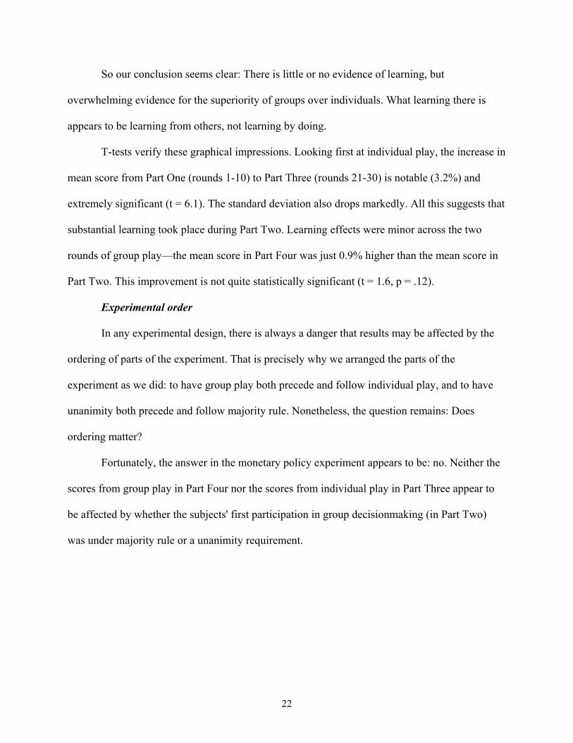
So our conclusion seems clear: There is little or no evidence of learning, but

overwhelming evidence for the superiority of groups over individuals. What learning there is

appears to be learning from others, not learning by doing.

T-tests verify these graphical impressions. Looking first at individual play, the increase in

mean score from Part One (rounds 1-10) to Part Three (rounds 21-30) is notable (3.2%) and

extremely significant (t = 6.1). The standard deviation also drops markedly. All this suggests that

substantial learning took place during Part Two. Learning effects were minor across the two

rounds of group play—the mean score in Part Four was just 0.9% higher than the mean score in

Part Two. This improvement is not quite statistically significant (t = 1.6, p = .12).

Experimental order

In any experimental design, there is always a danger that results may be affected by the

ordering of parts of the experiment. That is precisely why we arranged the parts of the

experiment as we did: to have group play both precede and follow individual play, and to have

unanimity both precede and follow majority rule. Nonetheless, the question remains: Does

ordering matter?

Fortunately, the answer in the monetary policy experiment appears to be: no. Neither the

scores from group play in Part Four nor the scores from individual play in Part Three appear to

be affected by whether the subjects' first participation in group decisionmaking (in Part Two)

was under majority rule or a unanimity requirement.

23

3. The Purely Statistical Experiment

3.1 Description of the Urn Experiment

Our second experiment placed subjects in a probabilistic environment devoid of any

economic content, but structured to capture salient features of monetary policy decisions

wherever possible.23 While such content-free problem solving may be of limited practical

relevance, our motive was to create an experimental setting into which students would carry little

or no prior intellectual baggage. While artificial in the extreme, this austere setup has at least one

important virtue: It allows us to isolate the pure effect of individual versus group

decisionmaking.

Specifically, the problem was a variant of the classic "urn problem" in which subjects

sample from an urn and then are asked to estimate its composition. In our application, groups of

five students were placed in front of computers which were programmed with electronic "urns"

consisting, initially, of 50% "blue balls" and 50% "red balls."

They were told that the composition of the urn would change to either 70% blue balls and

30% red balls, or to 70% red and 30% blue, at some randomly-selected point in the experiment.

Subjects were not told when the change would take place, nor in which direction—in fact, the

latter is what they were asked to guess. But we did inform students of the probability law that

governed the timing of the color change: The change was equally likely to occur just prior to any

of the first 10 draws and would definitely occur no later than the 10th.24

We once again provided subjects with a clear objective function so that we could

unambiguously distinguish better decisions from worse ones. This objective function weighed

23 Actually, we conducted the urn experiment first. We report them in reverse order because the monetary policy experiment is more interesting substantively. 24 Random number generators determined both the direction of the change and its timing. Sampling was with replacement.

24

the two criteria on which the quality of decisionmaking would be judged—speed and accuracy—

as follows. Subjects began each round with 40 points "in the bank" and could earn another 60

points by correctly guessing the direction in which the urn's composition changed.25 Subjects

were allowed to draw as many "balls" as they wished before making their guess—up to an upper

limit of 40, which was rarely reached.26 However, they paid a penalty of one point for each draw

they made after the urn changed composition, but before they guessed the majority color. (Call

this the decision lag, L.) For example, if the composition changed on the 8th draw, and the

subject guessed correctly after the 15th draw, L would be equal to 7, and the score for that round

would be 40 + 60 − 7 = 93. If the guess was incorrect, the score would be 40 − 7 = 33. A similar

penalty was assessed if the subject guessed the composition before the change took place (a

negative decision lag). Thus, if the composition of the urn was programmed to change on the 8th

draw, but the guess came after the 4th, the subject would be penalized 4 points for guessing too

soon. In sum, the objective function was:

(4) S = 40 + 60C − L,

where:

S = score (0-100 scale)

C ( a dummy variable) = 1 if guess is correct

= 0 if guess is incorrect

L = decision lag = T – N

T = the draw on which the composition changed (a random integer drawn from a uniform

distribution on [1,10])

N = the draw after which the subject guessed the composition of the urn. 25 Points were later converted into money at a rate known to the students: 500 points = $1. 26 In almost 4200 plays of the game, this upper limit was hit only five times.

25

Before going further, a few remarks on the structure of the experiment are in order. First,

while the entire setup was devoid of substantive content, it was designed to evoke the nature of

monetary policy decisionmaking. For example, policymakers never know for sure when

macroeconomic conditions (analogous to the urn's composition) call for a change in monetary

policy (a declaration that the composition has changed). Instead, they gradually receive more and

more information (more drawings from the urn) suggesting that a change in policy may make

sense. Eventually, enough such data accumulate and policy is changed. Nor does anyone tell the

central bank whether policy should be tightened or eased. (Is the urn now 70% red or 70% blue?)

In principle, after the arrival of each new piece of data (after each drawing), policymakers ask

themselves whether to adjust policy now or wait for more information—which is precisely what

our student subjects had to do.

Second, changes in the color ratio from 50%-50% to 70%-30% are pretty easy to detect,

but not "too easy."27 Again, this aspect of the experimental design was meant to evoke the

problem faced by monetary policymakers. Rarely are central bankers in a quandary over whether

they should tighten or ease. The policy debate is usually over whether to tighten or do nothing, or

over whether to ease or do nothing.

Third, the ratio 60:1 in the objective function determines the relative values of being

accurate (60 points for getting the composition right) versus being fast (each additional draw

costs 1 point). This ratio was set so high for two reasons. One is that it seems to us that

accuracy—that is, getting the direction right—is vastly more important than speed in the

monetary policy context. The other reason was that experimentation with this parameter taught

27 This is a probabilistic statement. It is certainly possible to draw, say, equal numbers of blue and red balls when the urn is, say, 70% red. Indeed, we saw this happen during the experiment.

26

us that quite a high ratio was needed to dissuade subjects from jumping the gun by guessing the

color too soon.

Fourth, 40 "free points" were provided on each round in order to make negative scores

impossible. The lowest possible score on any round—1 point—would be obtained by guessing

incorrectly after 40 drawings when the change in composition occurred on the 1st draw.

The game was played as follows. Subjects were given and read detailed instructions

(shown in the appendix) and then allowed to practice with the computer apparatus and ask

questions for about five minutes. As in the monetary policy experiment, scores during those

practice rounds were displayed but not recorded. At the end of the practice period, each student

was instructed to play 10 rounds of the game alone—without communicating with the other

students. Subjects proceeded at their own pace; clock time was again irrelevant. When all five

subjects had completed 10 rounds, the experimenter called a halt to Part One of the experiment.28

In Part Two, the five students played the same game 30 times as a group. The rules were

exactly the same, except that students were now permitted to communicate freely. During group

play, all five students received the group's common scores. We ran 20 sessions in all, involving

100 subjects. Just as in the monetary policy experiment, decisions in Part Two were made by

majority rule in half of the sessions and unanimously in the other half.

After 30 rounds of group play, the subjects returned to their individual machines for Part

Three, in which they played the game another 10 times alone. Following that, they returned to

the group computer for Part Four, in which decisions were now made unanimously if they had

been by majority rule in Part Two, or by majority rule if they had previously been under

28 The experimenters were Blinder and Morgan for the first few sessions, and then a graduate student, Felix Vardy, for the rest. In the urn experiment, we found that while qualitative results were unaffected by the identity of the experimenter, there was a significant level effect in scores: subjects on average did worse in the first two sessions

27

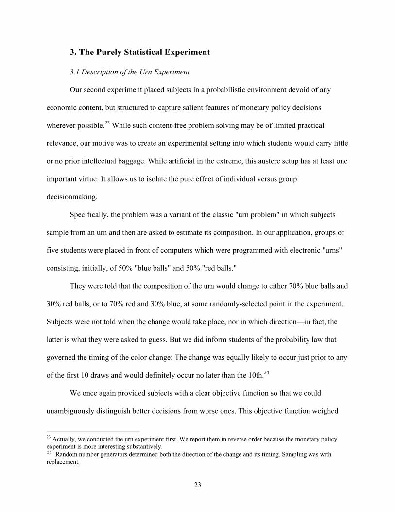
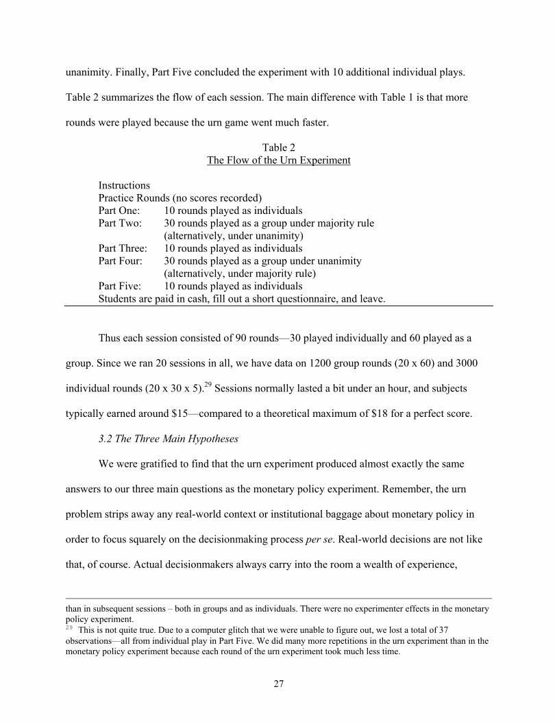
unanimity. Finally, Part Five concluded the experiment with 10 additional individual plays.

Table 2 summarizes the flow of each session. The main difference with Table 1 is that more

rounds were played because the urn game went much faster.

Table 2 The Flow of the Urn Experiment

Instructions Practice Rounds (no scores recorded) Part One: 10 rounds played as individuals Part Two: 30 rounds played as a group under majority rule

(alternatively, under unanimity) Part Three: 10 rounds played as individuals Part Four: 30 rounds played as a group under unanimity

(alternatively, under majority rule) Part Five: 10 rounds played as individuals Students are paid in cash, fill out a short questionnaire, and leave.

Thus each session consisted of 90 rounds—30 played individually and 60 played as a

group. Since we ran 20 sessions in all, we have data on 1200 group rounds (20 x 60) and 3000

individual rounds (20 x 30 x 5).29 Sessions normally lasted a bit under an hour, and subjects

typically earned around $15—compared to a theoretical maximum of $18 for a perfect score.

3.2 The Three Main Hypotheses

We were gratified to find that the urn experiment produced almost exactly the same

answers to our three main questions as the monetary policy experiment. Remember, the urn

problem strips away any real-world context or institutional baggage about monetary policy in

order to focus squarely on the decisionmaking process per se. Real-world decisions are not like

that, of course. Actual decisionmakers always carry into the room a wealth of experience,

than in subsequent sessions – both in groups and as individuals. There were no experimenter effects in the monetary policy experiment. 29 This is not quite true. Due to a computer glitch that we were unable to figure out, we lost a total of 37 observations—all from individual play in Part Five. We did many more repetitions in the urn experiment than in the monetary policy experiment because each round of the urn experiment took much less time.

28

knowledge, prejudices, etc. Certainly, that is true of monetary policymakers. To find the same

results in these two very different contexts gives us some confidence in the robustness of our

results.

Now to the specifics. Remember, our first and most crucial hypothesis was:

H1: Groups decisions are more inertial than individual decisions.

In the monetary policy experiment, the average lag was actually shorter for the groups,

but not significantly so. In the urn experiment, the two means were again not significantly

different at conventional levels (t=1.1), even with thousands of observations. But this time the

average lag was indeed longer for the groups: 6.60 draws versus 6.40 draws for individuals.

Histograms for the variable L (the decision lag) in individual and group play once again look

strikingly alike. (See Figure 2.) Again, the left-hand panel looks like a mean-preserving spread

on the right-hand panel.

Individual Play Group Play

Fra

ctio

n

lag-10 0 10 20 30 40

0

.1

.2

.3

.4

Fra

ctio

n

lag-10 0 10 20 30 40

0

.1

.2

.3

.4

Figure 3: Histograms of Lag in Urn Experiment

29

Since each experimental session always started with individual play, we can again ask

whether learning-by-doing might have clouded the comparison. To examine this possibility, we

began by comparing the individual decisions made in Part Three of the game (rounds 41-50)—

when learning is presumably over—with group decisions in the ten preceding rounds and the ten

following rounds. Compared to group play in Part Two, individual decisions are a bit slower

(6.56 versus 6.26), but again the difference is not significant (t = 0.75). The ten group rounds in

Part Four exhibited a slightly greater mean lag (6.65), but the difference is also not significant (t

= 0.17). The same conclusions hold if we treat each session as a single observation. In only 12

of 20 sessions did the average group lag exceed the average individual lag. Using the Wilcoxon

signed-ranks test, we cannot reject the null hypothesis that there is no difference in the mean lags

against the one-sided alternative that group lags exceed individual lags. The test statistic is just

0.6, which is not significant at conventional levels.

The overall conclusion, then, is the same one that we reached in the first experiment:

groups are not more inertial in their decision making than are individuals.30

H2: Groups make better decisions than individuals.

Our second hypothesis pertains to quality rather than the speed. Do groups make better

decisions than individuals? As was the case in the monetary policy experiment, the experimental

data generated by the urn experiment strongly support the hypothesis that groups outperform

individuals. The quality of the decision is measured unambiguously by the variable S ("score")

defined in equation (4). In the overall sample, the average score attained by groups was 86.8 (on

a 1-100 scale), versus only 83.7 for individuals. The difference is highly significant statistically

30 As noted earlier, we define "more slowly" in this context as requiring more drawings before reaching a decision, not as taking more clock time.

30

(t = 4.3). More important, it seems large enough to be economically meaningful: Groups did

3.7% better, on average.31

The 3.7% performance gap between groups and individuals almost exactly matches what

we found in the monetary policy experiment (a 3.5% gap). We were surprised to find essentially

the same average performance improvement in two such different experimental settings. Even if

we had tried to "rig the deck" to make the two performance gaps come out the same, we would

have had no idea how to do so.

We illustrate the robustness of this conclusion in two ways. First, we once again go to the

extreme of treating the session as the unit of observation—leaving us with only 20 matched pairs

of individual and group observations. We can then test the null hypothesis that individual and

group scores are equal against the one-sided alternative given in Hypothesis 2. In 16 of the 20

sessions, the average group score exceeded the average individual score. Using a Wilcoxon

signed-ranks test, we obtain a z statistic of 3.2, which rejects the null hypothesis in favor of

Hypothesis 2 at any conventional significance level—despite having only 20 observations.

Second, to control for possible learning effects, we repeat what we did earlier for

Hypothesis 1: We compare individual decisions made in Part Three (when learning is

presumably over) with group decisions in the ten preceding and ten following rounds. Compared

to the ten preceding rounds in Part Two, group scores are about 3.8% better; and this difference

is significant (t = 2.0) at conventional levels. Comparing Parts Three and Four, groups scores are

still 2.3% above individual scores; but now the difference is no longer significant (t = 1.2). Still,

the overall conclusion supports the notion that groups outperform individuals.

Obviously, since the mean lags are statistically indistinguishable, the groups must have

acquired their overall edge through accuracy rather than through speed. Specifically, groups

31 That difference is about 72% of the standard deviation across individual mean scores.

31

guessed the urn's composition correctly 89.3% of the time whereas individuals got the color right

only 84.3% of the time. Considering that the experimental apparatus was set up to make guessing

the correct composition relatively easy, this gap of 5 percentage points is sizable. Look at it this

way: The error rate (frequency of guessing the wrong color) was 15.7% for individuals, but only

10.7% for groups. This difference in performance is also statistically significant (t = 4.2 with

individual observations and z = 1.9 when the session is treated as the unit of observation).

Finally, the margin of superiority of groups over individuals on this criterion (5.0 percentage

points) is strikingly similar to what we found in the monetary policy experiment (6.2 percentage

points).

However, the gap in accuracy does drop after the initial rounds of the experiment. The

error rate in Part Three (individual rounds 41-50) is still around 5% higher than in the ten group

rounds in Part Two (t = 1.8), but is only around 3% higher than in the ten group rounds in Part

Four (t = 1.2).

In brief, we find that group decisions in the urn experiment are more accurate without

being slower—just as we found in the monetary policy experiment.

H3: Decisions by majority rule are less inertial than decisions under a unanimity

requirement.

As noted earlier, we were surprised to find almost no differences between groups

operating under majority rule and groups operating under the unanimity principle in the

monetary policy experiment. In fact, contrary to our priors, decisions were made slightly faster

under the unanimity requirement. Thus, in the urn experiment, we expected no differences—

which is just what we found.

32

In fact, and quite surprisingly, decisions under the unanimity requirement were actually

made faster, on average, than decisions under majority rule (mean L = 6.34 versus 6.85). The

difference is actually significant at the 5% level in a one-tail test.32 However, there was no

significant difference between the two group treatments in either decisionmaking accuracy (C) or

quality (S). The composition of the urn was guessed correctly 89.2% of the time under majority

rule and 89.5% of the time under unanimity. On balance, we still feel comfortable pooling the

data from the majority-rule and unanimity treatments.

3.3 Other Results

Learning

Since the urn game is rather cumbersome to describe in words, but is extremely easy to

play "once you get the hang of it," we did expect to find learning effects, at least in the early

rounds. (Remember, there were no learning-by-doing effects in the monetary policy game.) Once

again, a graph probably summarizes the learning results best.

Figure 4 is constructed just like Figure 2. We again partitioned the data by round,

reflecting the chronological order of play. In the urn experiment, there were 90 rounds in each

session—30 played as individuals and 60 played as groups (see Table 2). So we have 100

observations (20 sessions times five individuals in each) on each of the first 10 rounds, 20

observations on each of rounds 11-40 (the 20 groups), and so on. Figure 4 displays the mean

score by round, and the horizontal lines indicate the means for each part of the experiment. The

vertical lines again indicate where subjects switched from individual to group decisionmaking, or

vice-versa.

32 If we treat the dataset as having just 20 observations, this difference is insignificant.

33

As we noted earlier, if there are systematic learning effects, scores should improve as we

progress through the rounds. In fact, the figure shows clear evidence of learning over the first 10-

12 rounds, but none thereafter. In addition, it is evident that average performance jumps upward

when we switch from individual to group play (the vertical lines at 10 and 50), and jumps

downward when we switch from group to individual play (the vertical lines at 40 and 80). All

four of these changes are statistically significant. In sum, the figure (and the related statistical

tests) suggest that learning occurred, but was limited to the early rounds and was dwarfed by the

difference in quality between individual and group decisions. Once again, these findings parallel

those in the monetary policy experiment.

It is natural to wonder whether learning mostly affects speed (the decisionmaking lag, L)

or accuracy (whether the urn's composition is guessed correctly, C). The answer is both, though

in different ways—as Figures 5 and 6 show. Interestingly, Figure 5, which displays the mean

decision lag, suggests the presence of learning throughout the experiment; there is a clear trend

Figure 4: Mean Score by Round in Urn Experiment

70

75

80

85

90

95

100

0 10 20 30 40 50 60 70 80 90

Round

Scor

e

Individual Individual Individual Group Group

34

toward waiting longer before guessing the dominant color.33 But Figure 6, which shows the

percentage of correct guesses, looks a lot like Figure 4—learning ends after the first 10-12

rounds. The reason is clear from equation (4): In computing the score, C (correct) gets 60 times

the weight of L (lag). Had we weighted L more heavily, a clearer indication of learning

throughout each session might have emerged.

33 We strongly believe that subjects tended to "jump the gun." So longer average lags are presumptively better. Indeed, several students observed that they learned to wait longer after playing as a group.

Figure 5: Mean Lag by Round in Urn Experiment

0

1

2

3

4

5

6

7

8

9

10

0 10 20 30 40 50 60 70 80 90

Round

Lag

Individual Individual Individual Group Group

35

Experimental Order

In the monetary policy experiment, we found no evidence that the order of group play

mattered. Unfortunately, there is a little evidence that it did in the urn experiment. In particular,

subjects performed significantly better in subsequent group play if their initial exposure to group

decisionmaking was under unanimity, rather than under majority rule.

Specifically, consider the scores obtained in the second 30 rounds of group play (600

observations from Part Four). If the groups played first under the unanimity rule and then under

majority rule, the mean score was 88.7. If the order was reversed, the mean score fell to 85.2.

The difference is significant by conventional standards (t = 2.4, p = 0.018), and we have no

explanation for it.34

Fortunately, this puzzling finding was not replicated in the individual data, so we are

inclined to treat it as a fluke. Parts Three and Five of individual play took place after the subjects'

Figure 6: Mean Percent Correct by Round in Urn Experiment

0.5

0.55

0.6

0.65

0.7

0.75

0.8

0.85

0.9

0.95

1

0 10 20 30 40 50 60 70 80 90

Round

Perc

ent C

orre

ct

Individual Individual Individual Group Group

36

first experience with group play. If their initial group experience was under unanimity, the

individual scores in subsequent rounds averaged 84.2; but if that initial group experience was

under majority rule, subsequent individual scores averaged 85.8. That difference, while not quite

significant (t = 1.8, p = .074), goes in the opposite direction from what we found for group play.

So, on balance, we are satisfied that experimental order does not have much of an effect on the

results.

4. Can We Model Group Decisionmaking?

It is possible to formulate and test several simple models of how groups aggregate

individual views into group decisions. None of these are strictly "economic" models, however,

because every homo economicus should make the same decision. (After all, both the objective

function and the information are identical for all participants.) As will be clear shortly, none of

these simple, intuitive models of group decisionmaking takes us very far.

Model 1: The whole is equal to the sum of its parts

The simplest model posits that there are no group interactions at all: The group's decision

is simply the average of the five individual decisions. This, of course, come closest to the pure

economic model (which says that everyone agrees). However, this model has, essentially,

already been tested and rejected in Sections 2 and 3. Let X denote any one of our three decision

variables (L, S, or C), and let XG be the average value attained by the group and XA be the

average values attained by the five people in the group when they played as individuals. As noted

earlier, we consistently reject XG = XA in favor of the alternative that groups do better.

34 Remember that, on average, there was no significant difference in scores between unanimity and majority rule.

37

Now let us ask a slightly different question: Looking across the 20 groups, does the

average performance of the five people who comprise a particular group (XA) take us very far in

explaining—in a regression sense—how well the group does on that same criterion (XG)? Since

we have three different choices of X (L, S, and C) and data from two different experiments, we

can pose six versions of this question. Rather than display the (rather unsuccessful) regression

equations, Figure 7 shows the corresponding scatter diagrams. Each is based on 20 observations,

one for each session. What message do these six charts convey?

38

Urn Experiment Monetary Policy Experiment

Gro

up

Sco

re

Individual Score - Average75 80 85 90 95

80

85

90

95

Figure 7: Group Compared to Average Individual Play

Gro

up

Pe

rce

nt

Co

rre

ct

Individual Percent Correct - Ave.75 .8 .85 .9 .95 1

.75

.8

.85

.9

.95

1

Gro

up

Sco

re

Individual Score - Average80 85 90 95

80

85

90

95

Gro

up

La

g

Individual Lag - Average0 2 4 6 8 10

0

2

4

6

8

10

Gro

up

La

g

Individual Lag - Average0 2 4 6 8 10

0

2

4

6

8

10

Gro

up

Pe

rce

nt C

orr

ect

Individual Percent Correct - Ave.75 .8 .85 .9 .95 1

.75

.8

.85

.9

.95

1

39

In general, they give the impression that a linear model of the form XG = a + bXA + u

does not fit the data at all well.35 In one case, the correlation is even negative. Looking across the

three variables, LA does by far the best job of explaining LG, although even here the simple

correlations are just 0.58 in the urn experiment and 0.57 in the monetary policy experiment—

corresponding to R2s of about 0.33. (The regression coefficients are 0.84 and 0.90, respectively.)

In the monetary policy experiment, the correlations for the other two variables, S and C, are

nearly zero.

In a word, the average performance of the five individuals who comprise each group

carries almost no explanatory power for how well the group performed. Most championship

sports teams would be surprised—and would be spending too much on payroll—if this were true

in professional sports.

Model 2: The median voter theory

A different concept of "average" plays a time-honored role in one of the few instances of

group decisionmaking that economists have modeled extensively: voting. Where preferences are

single-peaked, as they must be in these applications, a highly-pedigreed tradition in public

finance holds that the views of the median voter should prevail. It seems natural, then, to ask

whether the performance of the median player can explain the performances of our 5-person

groups? Remember, we literally used either a majority vote or a unanimous vote to determine the

group's decisions in our experiments.

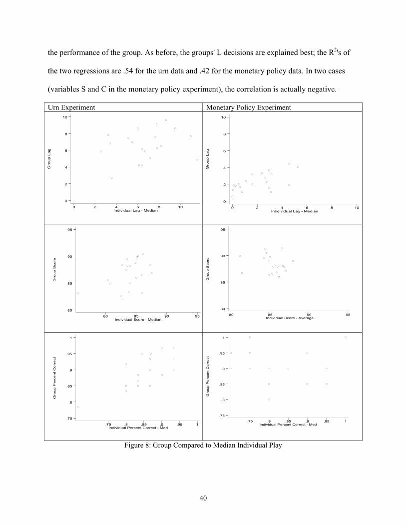
Figure 8, which follows the same format as Figure 7, shows that the median voter model

generally (but not always) is a better predictor of group outcomes than simple averaging. In one

case, the R2 gets as high as .54. But, in general, these six scatters once again show that even the

median-voter model has only modest success (and, in some cases, no success at all) in explaining

35 It is apparent from the diagrams that linearity is not the issue. No obvious nonlinear model does much better.

40

the performance of the group. As before, the groups' L decisions are explained best; the R2's of

the two regressions are .54 for the urn data and .42 for the monetary policy data. In two cases

(variables S and C in the monetary policy experiment), the correlation is actually negative.

Urn Experiment Monetary Policy Experiment

Figure 8: Group Compared to Median Individual Play

Gro

up

Pe

rce

nt

Co

rre

ct

Individual Percent Correct - Med.75 .8 .85 .9 .95 1

.75

.8

.85

.9

.95

1

Gro

up

Sco

re

Individual Score - Average80 85 90 95

80

85

90

95

Gro

up L

ag

Inbdividual Lag - Median0 2 4 6 8 10

0

2

4

6

8

10

Gro

up

La

g

Individual Lag - Median0 2 4 6 8 10

0

2

4

6

8

10

Gro

up

Sco

re

Individual Score - Median80 85 90 95

80

85

90

95

Gro

up

Pe

rce

nt

Co

rre

ct

Individual Percent Correct - Med.75 .8 .85 .9 .95 1

.75

.8

.85

.9

.95

1

41

Model 3: May the best man (or woman) win

In discussing our experiment with other economists, several suggested that the group's

decisions would be dominated by the best player in the group—as indicated, presumably, by his

or her scores while playing alone.36 This hypothesis struck us as plausible. So we tested models

of the form XG = a + bX* + u, where X* is the average outcome (on variable S, C, or L) of the

individual who achieved the highest average score while playing alone.

There is, however, a logically prior question: Are there statistically significant individual

fixed effects that can be used to identify "better" and "worse" players? To answer this question,

we ran a series of regressions, one for each experimental session, explaining individual scores by

five dummy variables, one for each player.37 Perhaps surprisingly, this preliminary test of the

idea that there is a "best player" turned up absolutely no evidence of reliable individual fixed

effects in the urn experiment: Only four of the 100 individual dummy variables were significant

at the 5% level. In the monetary policy experiment, however, there was some weak evidence that

some players are better and others worse: 15 of the 100 individual dummies were significant at

the 5% level.

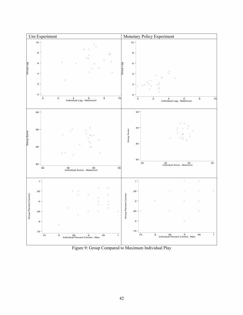
With this in mind, we can now look at Figure 9, which displays the six scatter diagrams.

In general, the fits appears to be quite modest. (The highest R2 among the six scatters is .28.) In

only one of the six cases (explaining CG in the monetary policy experiment), is this the best-

fitting model; in three cases, it is the worst. Once again, the variable L is explained best.

36 The subject pool was very close to 50% male and 50% female. 37 Thus each regression was based on 150 observations in the urn experiment and 100 observations in the monetary policy experiment.

42

Urn Experiment Monetary Policy Experiment

Figure 9: Group Compared to Maximum Individual Play

Gro

up

Sco

re

Individual Score - Maximum80 85 90 95

80

85

90

95

Gro

up P

erc

ent

Corr

ect

Individual Percent Correct - Max.75 .8 .85 .9 .95 1

.75

.8

.85

.9

.95

1

Gro

up

La

g

Individual Lag - Maximum0 2 4 6 8 10

0

2

4

6

8

10

Gro

up L

ag

Individual Lag - Maximum0 2 4 6 8 10

0

2

4

6

8

10

Gro

up

Sco

re

Individual Score - Maximum80 85 90 95

80

85

90

95

Gro

up

Pe

rce

nt

Co

rre

ct

Individual Percent Correct - Max.75 .8 .85 .9 .95 1

.75

.8

.85

.9

.95

1

43

Finally, we note that various multiple regressions using, say, both XA and X* do not

appreciably improve the fit. In the end, we are left to conclude that neither the average player,

nor the median player, nor the best player determine the decisions of the group. The whole, we

repeat, does indeed seem to be something different from—and generally better than—the sum of

its parts.

5. Conclusions

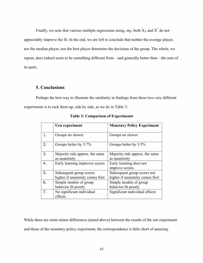
Perhaps the best way to illustrate the similarity in findings from these two very different

experiments is to rack them up, side by side, as we do in Table 3:

Table 3: Comparison of Experiments

Urn experiment Monetary Policy Experiment

1. Groups no slower Groups no slower

2. Groups better by 3.7% Groups better by 3.5%

3. Majority rule approx. the same as unanimity

Majority rule approx. the same as unanimity

4. Early learning improves scores Early learning does not improve scores

5. Subsequent group scores higher if unanimity comes first

Subsequent group scores not higher if unanimity comes first

6. Simple models of group behavior fit poorly

Simple models of group behavior fit poorly

7. No significant individual effects

Significant individual effects

While there are some minor differences (noted above) between the results of the urn experiment

and those of the monetary policy experiment, the correspondence is little short of amazing.

44

From the start, our interest centered on the first two findings:

* Do groups reach decisions more slowly than individuals? According to these

experimental results, groups appear to be no slower in reaching decisions than individuals are.

* Do groups make better decisions than individuals? The experimental answer seems to

be yes. And the margin of superiority of group over individual decisions is astonishingly similar

in the two experiments—about 3 1/2%.

If groups make better decisions and require no more information to do so, then two

heads—or, in this case, five—are indeed better than one. Society is, in that case, wise to assign

many important decisions, like monetary policy, to committees.

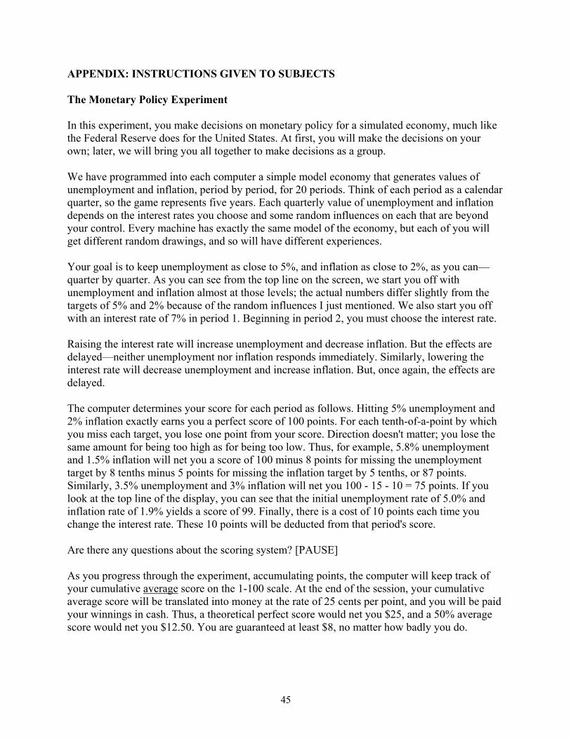
45

APPENDIX: INSTRUCTIONS GIVEN TO SUBJECTS

The Monetary Policy Experiment In this experiment, you make decisions on monetary policy for a simulated economy, much like the Federal Reserve does for the United States. At first, you will make the decisions on your own; later, we will bring you all together to make decisions as a group. We have programmed into each computer a simple model economy that generates values of unemployment and inflation, period by period, for 20 periods. Think of each period as a calendar quarter, so the game represents five years. Each quarterly value of unemployment and inflation depends on the interest rates you choose and some random influences on each that are beyond your control. Every machine has exactly the same model of the economy, but each of you will get different random drawings, and so will have different experiences. Your goal is to keep unemployment as close to 5%, and inflation as close to 2%, as you can—quarter by quarter. As you can see from the top line on the screen, we start you off with unemployment and inflation almost at those levels; the actual numbers differ slightly from the targets of 5% and 2% because of the random influences I just mentioned. We also start you off with an interest rate of 7% in period 1. Beginning in period 2, you must choose the interest rate. Raising the interest rate will increase unemployment and decrease inflation. But the effects are delayed—neither unemployment nor inflation responds immediately. Similarly, lowering the interest rate will decrease unemployment and increase inflation. But, once again, the effects are delayed. The computer determines your score for each period as follows. Hitting 5% unemployment and 2% inflation exactly earns you a perfect score of 100 points. For each tenth-of-a-point by which you miss each target, you lose one point from your score. Direction doesn't matter; you lose the same amount for being too high as for being too low. Thus, for example, 5.8% unemployment and 1.5% inflation will net you a score of 100 minus 8 points for missing the unemployment target by 8 tenths minus 5 points for missing the inflation target by 5 tenths, or 87 points. Similarly, 3.5% unemployment and 3% inflation will net you 100 - 15 - 10 = 75 points. If you look at the top line of the display, you can see that the initial unemployment rate of 5.0% and inflation rate of 1.9% yields a score of 99. Finally, there is a cost of 10 points each time you change the interest rate. These 10 points will be deducted from that period's score. Are there any questions about the scoring system? [PAUSE] As you progress through the experiment, accumulating points, the computer will keep track of your cumulative average score on the 1-100 scale. At the end of the session, your cumulative average score will be translated into money at the rate of 25 cents per point, and you will be paid your winnings in cash. Thus, a theoretical perfect score would net you $25, and a 50% average score would net you $12.50. You are guaranteed at least $8, no matter how badly you do.

46

The game works as follows. You can move the interest rate up or down, in increments of 1 percentage point, by clicking on the up or down buttons on the left-hand side of the screen, or by moving the slide bar. Try that now to see how it works. When you have selected the interest rate you want, click on the button marked "Click to Set Rate." Do that now. The computer has recorded your interest rate choice, drawn the random numbers I mentioned earlier, and calculated that period's unemployment, inflation, and score. There is one final, important aspect to the game. In a time period selected at random, but equally likely to be any of the first 10 periods, aggregate demand will either increase or decrease. You will not be told when this happens nor in which direction. If aggregate demand increases, that tends to push unemployment down and, with a lag, inflation up. If aggregate demand decreases, that tends to push unemployment up and, with a lag, inflation down. The essence of your job is to figure out when and how to adjust monetary policy in order to keep unemployment as close to 5%, and inflation as close to 2%, as possible. Remember, the change in aggregate demand will come at a randomly selected time within the first 10 periods; and we will not tell you whether demand has gone up or down. Further, each interest rate change will cost you 10 points in the period you make it. Are there any questions? This will all be simpler once you've practiced on the apparatus a bit. You can do so now, and the scores you see will just be displayed for your information; they will not be recorded or counted. You can practice for about 5 to 10 minutes to develop some familiarity with how the game works. During this practice time, feel free to ask any questions you wish. [AFTER PRACTICE] OK, it's time to start the game for real now. In this part of the experiment, you will play the monetary policy game 10 times by yourselves. You may not communicate with any other player, and the points you earn will be your own. After you have played the game 10 times, the computer will prevent you from going on. Please start now. Proceed at you own pace. [AFTER PART ONE] Good. Now please gather around this computer to play the same game as a group. [PAUSE] In this part of the experiment, you will play exactly the same game 10 times. The rules are the same except that decisions are now made by majority rule. I will control the mouse, and will not do anything until at least three of you have agreed. You may communicate freely with each other, as much and in any way you wish. While playing as a group, you each receive the group's score. Any questions? [AFTER PART TWO] OK. Now please return to your individual seats and, once again, play 10 more rounds of the game by yourselves. Communication with other players is not allowed. The computer will again stop you after 10 rounds.

47

[AFTER PART THREE] This is the last part of the experiment. Now let's gather around the group computer again to play the game together. This part of the experiment is the same as the previous group play except that decisions must now be unanimous. I will not do anything until all of you have agreed on a common decision. As before, feel free to communicate in any way you wish. In this part of the experiment, which will last 10 rounds, you will each once again receive the group's score. Any questions?

The Urn Experiment Thank you for volunteering for this experiment about decisionmaking. We have set up, on these computers, a controlled environment in which there are objectively “better” and “worse” decisions. As I will explain shortly, you will be paid according to how good your decisions are. The higher your score, the more you earn. As you can see, there are five people participating in this experiment; the same instructions apply equally all. The experiment consists of five parts. In three of the five parts, you will play the game by yourself, at your own computer. During those parts, please do not talk or in any way communicate with other people. In two of the five parts, you will all play the game together. Then you may freely communicate, as much as you wish. In each round, you will earn points which will later be converted into money at the rate of 500 points to one dollar. At the end of the experiment, you will be paid what you have earned in all rounds, in cash. Since there are 90 rounds in total, and the maximum amount you can earn in each round is 20 cents, the theoretical maximum you could earn—with a perfect score—is $18. Description of each round The goal in each round is the same: to guess correctly the number of red or blue balls in a simulated urn, and when the number of balls changes. Specifically, each time you click on the DRAW AGAIN button, the computer will draw a ball from a simulated urn containing 100 balls. Initially, 50 of the balls are red and 50 are blue. Balls are placed back in the urn after each drawing. Go ahead and try that now—as you see, you have drawn a blue ball. Just before some randomly selected drawing, equally likely to be any of the first ten, the computer will change the composition of the urn either to 70 red balls and 30 blue balls or to 30 red and 70 blue balls. Either change is equally likely, and you will be told neither when the change happens nor the direction of the change. But you do know for sure that some change will

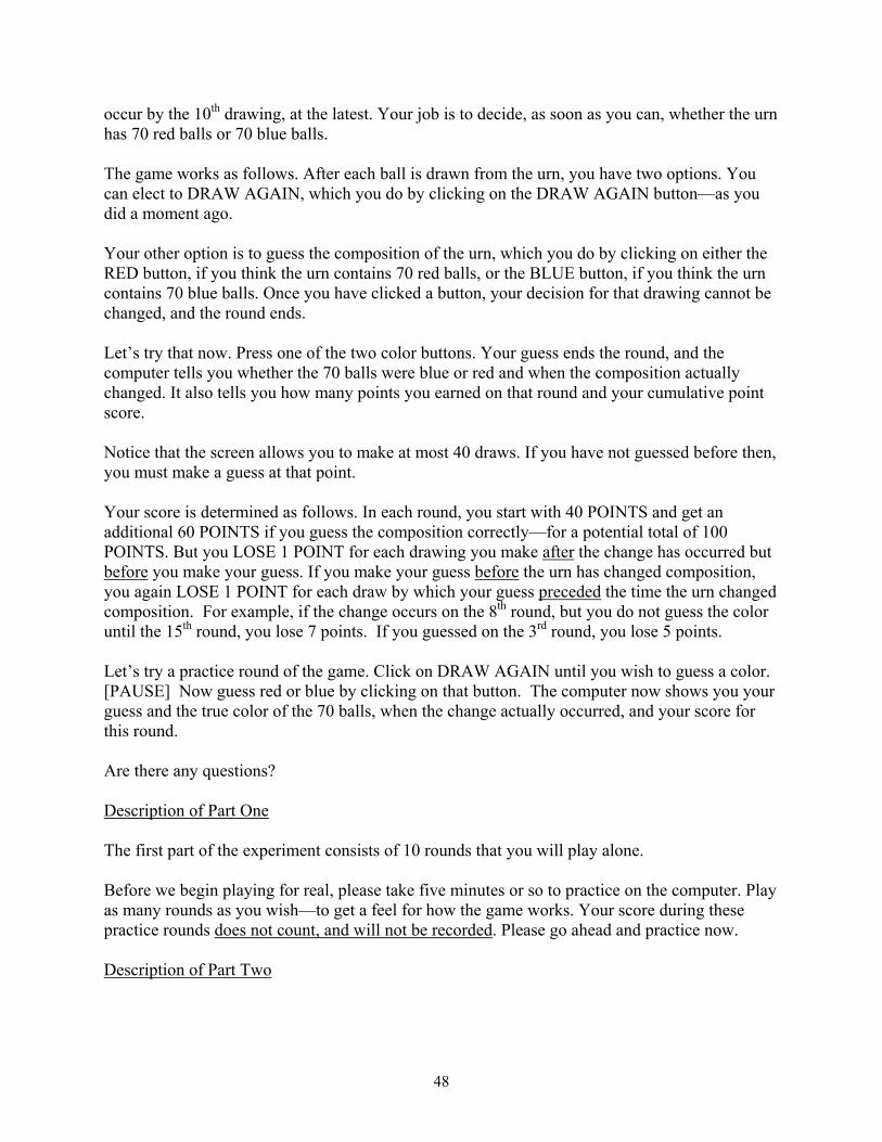
48

occur by the 10th drawing, at the latest. Your job is to decide, as soon as you can, whether the urn has 70 red balls or 70 blue balls. The game works as follows. After each ball is drawn from the urn, you have two options. You can elect to DRAW AGAIN, which you do by clicking on the DRAW AGAIN button—as you did a moment ago. Your other option is to guess the composition of the urn, which you do by clicking on either the RED button, if you think the urn contains 70 red balls, or the BLUE button, if you think the urn contains 70 blue balls. Once you have clicked a button, your decision for that drawing cannot be changed, and the round ends. Let’s try that now. Press one of the two color buttons. Your guess ends the round, and the computer tells you whether the 70 balls were blue or red and when the composition actually changed. It also tells you how many points you earned on that round and your cumulative point score. Notice that the screen allows you to make at most 40 draws. If you have not guessed before then, you must make a guess at that point. Your score is determined as follows. In each round, you start with 40 POINTS and get an additional 60 POINTS if you guess the composition correctly—for a potential total of 100 POINTS. But you LOSE 1 POINT for each drawing you make after the change has occurred but before you make your guess. If you make your guess before the urn has changed composition, you again LOSE 1 POINT for each draw by which your guess preceded the time the urn changed composition. For example, if the change occurs on the 8th round, but you do not guess the color until the 15th round, you lose 7 points. If you guessed on the 3rd round, you lose 5 points. Let’s try a practice round of the game. Click on DRAW AGAIN until you wish to guess a color. [PAUSE] Now guess red or blue by clicking on that button. The computer now shows you your guess and the true color of the 70 balls, when the change actually occurred, and your score for this round. Are there any questions? Description of Part One The first part of the experiment consists of 10 rounds that you will play alone. Before we begin playing for real, please take five minutes or so to practice on the computer. Play as many rounds as you wish—to get a feel for how the game works. Your score during these practice rounds does not count, and will not be recorded. Please go ahead and practice now. Description of Part Two

49

In the second part of the experiment, you will make decisions as a group. So let’s all move to these seats over here. [WAIT] In this part, all decisions must be made by majority rule, and everyone in the group gets the same score. You may speak with each other freely, as often as you wish. After each drawing, the group must tell [NAME] whether to DRAW AGAIN or choose RED or BLUE, just as in the first part of the experiment. [NAME] will not do anything until you all agree. We will play this version of the game for 30 rounds. Description of Part Three In the next part of the experiment, you will again play 10 rounds of the game alone, just as you did in part one. Description of Part Four In this part of the experiment, you will again play the game together as a group. But this time, decisions must be made unanimously. Otherwise, the rules are exactly the same as before: We will play 30 rounds, you may talk as much as you wish, and everyone gets the same score. Description of Part Five In this last portion of the game, you return again to your original seats and play the game alone 10 more times. When you finish, the computer will tell you how much you have earned.

50

REFERENCES

Kenneth J. Arrow, Social Choice and Individual Values (New York: Wiley), 1963.

Laurence Ball, "Efficient Rules for Monetary Policy," NBER Working Paper No. 5952, March

1997.

Alan S. Blinder, Central Banking in Theory and Practice (Cambridge: MIT Press), 1998.

Alan S. Blinder, The Quiet Revolution: Central Banking Goes Modern (New Haven, Conn.:

Yale University Press, forthcoming 2003).

Gary Bornstein and Ilan Yaniv, “Individual and group behavior in the ultimatum game: Are

groups more ‘rational’ players?” Experimental Economics, 1 (1998), 101-8.

Timothy N. Cason and Vai-Lam Mui, “A laboratory study of group polarization in the team

dictator game,” Economic Journal, 107 (1997), 1465-83.

James C. Cox and Stephen C. Hayne, “Group versus individual decision making in strategic

market games,” mimeo, University of Arizona, 1998.

H. Gersbach and V. Hahn, “Voting Transparency and Conflicting Interests in Central Bank

Councils,” Deutsche Bundesbank Economic Research Center Discussion Paper 03/01, January

2001.

Norbert L. Kerr, Robert J. MacCoun, and Geoffrey P. Kramer, “Bias in judgment: comparing

individuals and groups,” Psychological Review, 103 (1996), 687-719.

Martin G. Kocher and Matthias Sutter, “When the ‘decision-maker’ matters: Individual versus

team behavior in experimental ‘beauty contest’ games,” Discussion Paper 2000/4, University of

Innsbruck, 2000.

Petra Kristen, “Monetary Policy Committees and Interest-Rate Setting, processed, University

of Basel, February 2001.

51

Marvin Goodfriend. “The Role of a Regional Bank in a System of Central Banks,” Federal

Reserve Bank of Richmond Economic Quarterly, Winter 2000, pp. 7-25.

J.P. Morgan & Co., Guide to Central Bank Watching, March 2000.

Glenn D. Rudebusch and Lars E.O. Svensson, "Policy Rules for Inflation Targeting," in J. B.

Taylor (ed.), Monetary Policy Rules (Chicago: University of Chicago Press), 1999, pp. 203-246.

M. A. Wallach, N. Kogan, and D. J. Bem, “Diffusion of responsibility and level of risk taking

in groups.” Journal of Abnormal Social Psychology, 68 (1964), 263-274.