1

Integration of Background Modeling and Object Tracking

Yu-Ting Chen, Chu-Song Chen, Yi-Ping Hung

IEEE ICME, 2006

2

Outline

Introduction General BG Modeling Description Variable Threshold Selection Experiment results Conclusion

3

Introduction (1/4) Background modeling:

Important for many applications: Visual surveillance. Human gesture analysis.

Moving object detection: BG and FG classification.

Method: Mixture of Gaussian distribution (in this

paper) Pixel-wise. Appropriate to dynamic BG.

4

Introduction (2/4)

Object tracking: Appearance model:

Color histogram is used (in this paper). Measure the similarity of the target

object and candidates. Search algorithm:

Find the most likely state of tracked object via similarity measurement.

Particle filtering is used (in this paper).

5

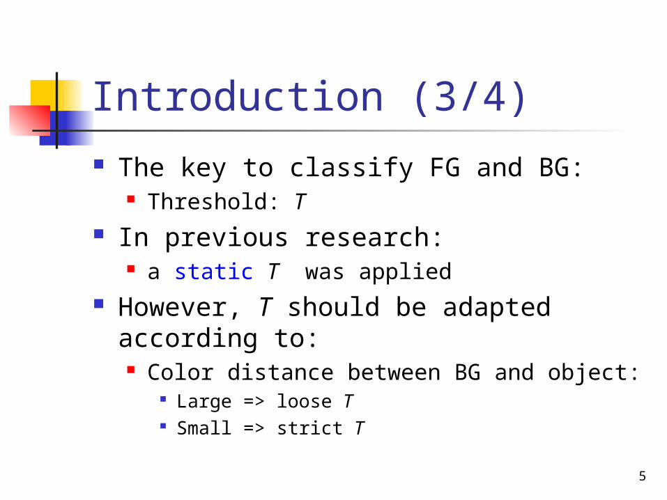
Introduction (3/4) The key to classify FG and BG:

Threshold: T In previous research:

a static T was applied However, T should be adapted

according to: Color distance between BG and object:

Large => loose T Small => strict T

6

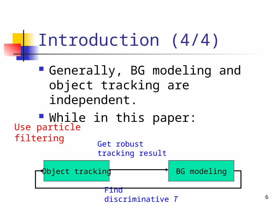
Introduction (4/4)

Generally, BG modeling and object tracking are independent.

While in this paper:

Object tracking BG modeling

Find discriminative T

Get robust tracking result

Use particle filtering

7

Outline

Introduction General BG Modeling Description Variable Threshold Selection Experiment results Conclusion

8

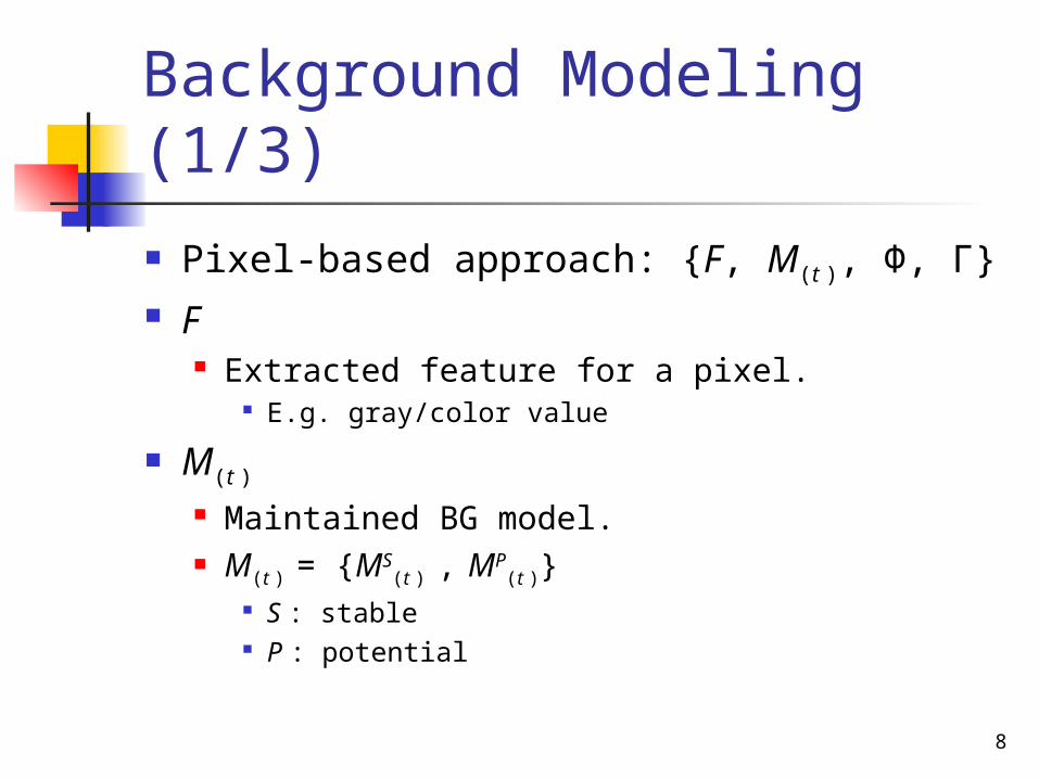
Background Modeling (1/3)

Pixel-based approach: {F, M(t ), Φ, Γ} F

Extracted feature for a pixel. E.g. gray/color value

M(t ) Maintained BG model. M(t ) = {MS

(t ) , MP(t )}

S : stable P : potential

9

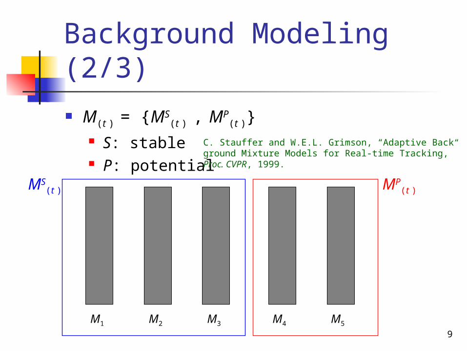
Background Modeling (2/3)

M(t ) = {MS(t ) , MP

(t )} S: stable P: potential

M1 M2 M3 M4 M5

MS(t ) MP

(t )

C. Stauffer and W.E.L. Grimson, “Adaptive Background Mixture Models for Real-time Tracking,” Proc. CVPR, 1999.

10

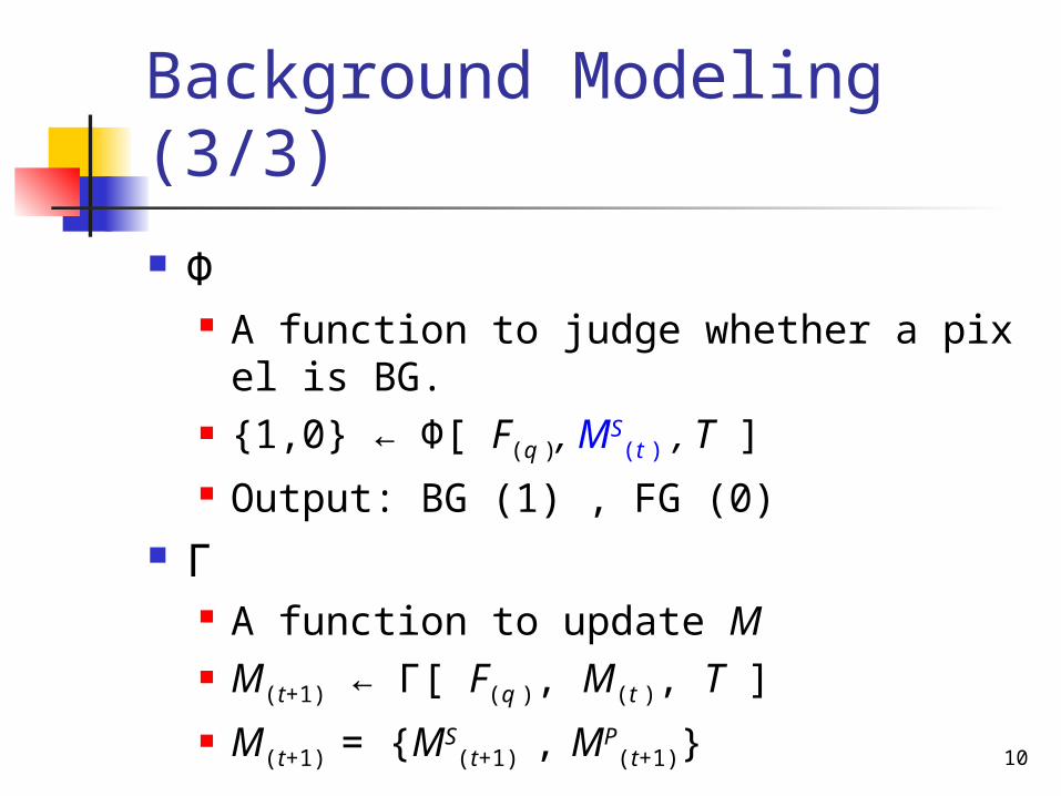
Background Modeling (3/3)

Φ A function to judge whether a pixel is BG. {1,0} ← Φ[ F(q ), MS

(t ) , T ] Output: BG (1) , FG (0)

Γ A function to update M M(t+1) ← Γ[ F(q ), M(t ), T ] M(t+1) = {MS

(t+1) , MP(t+1)}

11

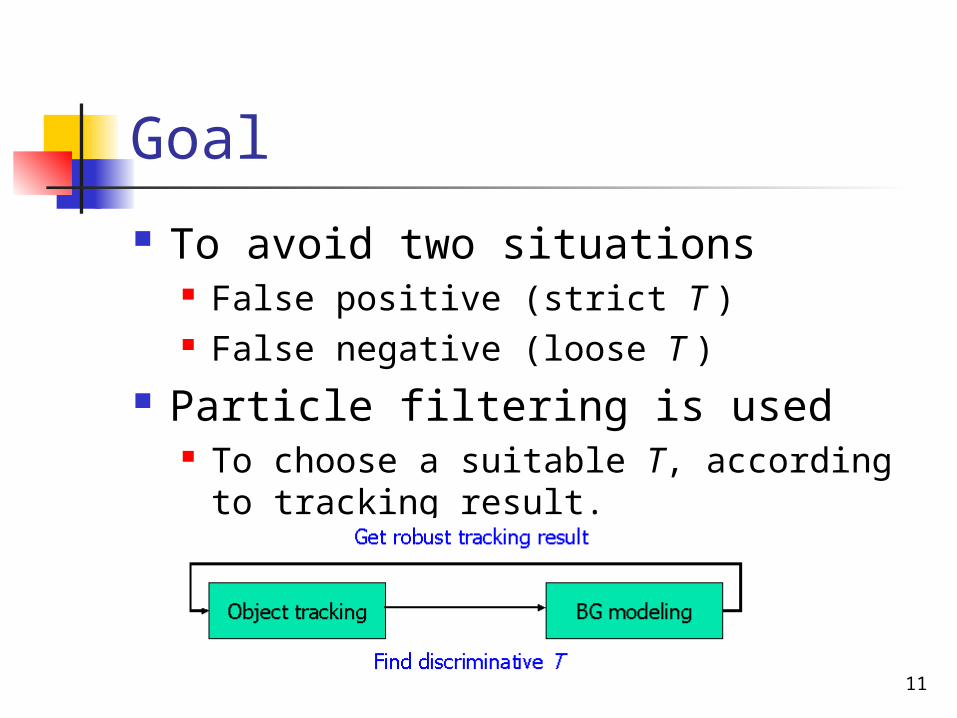
Goal

To avoid two situations False positive (strict T ) False negative (loose T )

Particle filtering is used To choose a suitable T, according to trackin

g result.

12

Outline

Introduction General BG Modeling Description Variable Threshold Selection Experiment results Conclusion

13

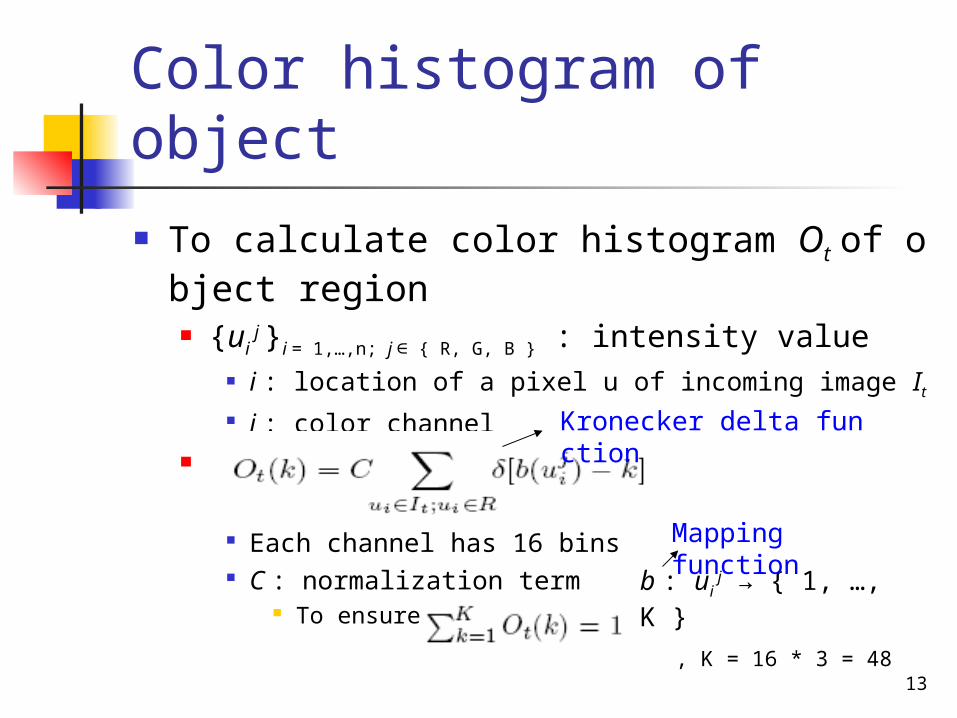
Color histogram of object

To calculate color histogram Ot of object region {ui

j }i = 1,…,n; j ∈ { R, G, B } : intensity value i : location of a pixel u of incoming image It j : color channel

Each channel has 16 bins C : normalization term

To ensure:

Kronecker delta function

b : ui j → { 1, …, K }

, K = 16 * 3 = 48

Mapping function

14

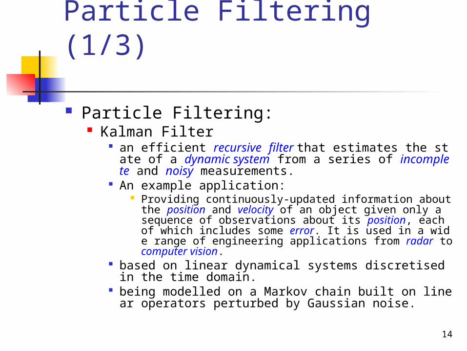
Particle Filtering (1/3)

Particle Filtering: Kalman Filter

an efficient recursive filter that estimates the state of a dynamic system from a series of incomplete and noisy measurements.

An example application: Providing continuously-updated information about the

position and velocity of an object given only a sequence of observations about its position, each of which includes some error. It is used in a wide range of engineering applications from radar to computer vision.

based on linear dynamical systems discretised in the time domain.

being modelled on a Markov chain built on linear operators perturbed by Gaussian noise.

15

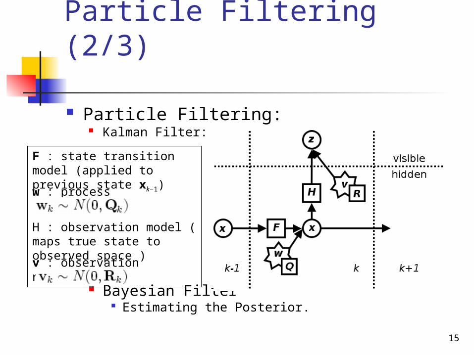
Particle Filtering (2/3)

Particle Filtering: Kalman Filter:

Bayesian Filter Estimating the Posterior.

F : state transition model (applied to previous state xk−1)w : process noise

H : observation model ( maps true state to observed space )v : observation noise

16

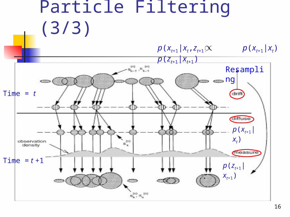
Particle Filtering (3/3)

Resampling

Time = t

Time = t +1

p(xt+1|xt)

p(zt+1|xt+1)

p(xt+1|xt,zt+1) p(xt+1|xt) p(zt+1|xt+1)

17

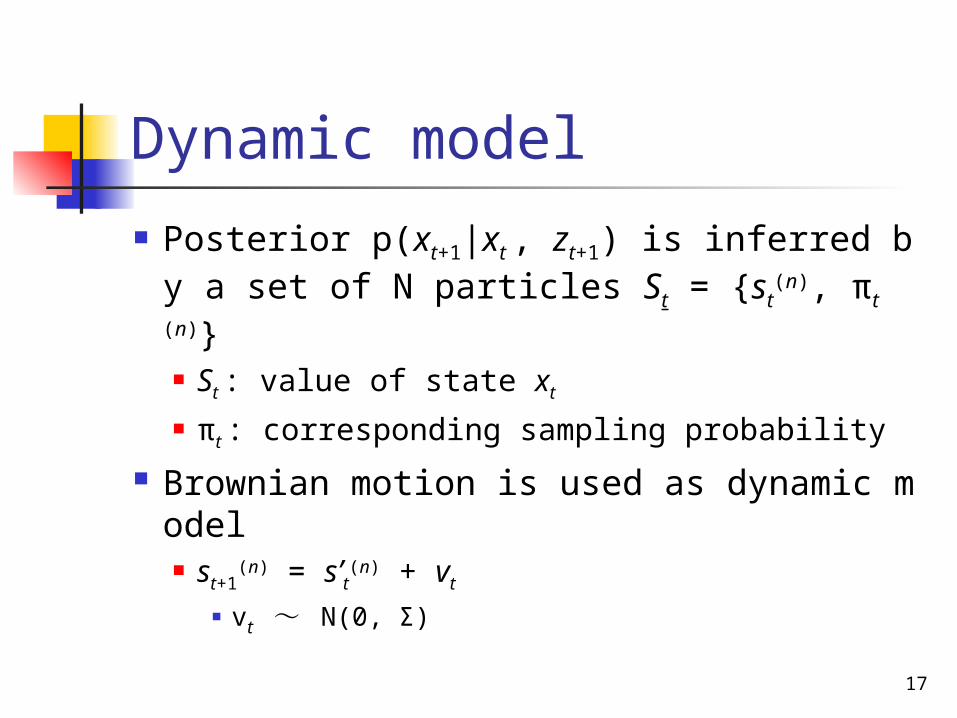
Dynamic model

Posterior p(xt+1|xt , zt+1) is inferred by a set of N particles St = {st

(n), πt(n)}

St : value of state xt

πt : corresponding sampling probability Brownian motion is used as dynamic mo

del st+1

(n) = s’t(n) + vt

vt ～ Ν(0, Σ)

18

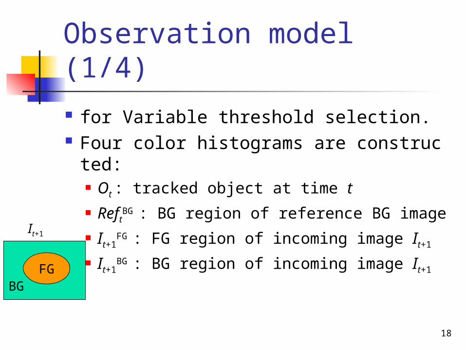
Observation model (1/4)

for Variable threshold selection. Four color histograms are constructe

d: Ot : tracked object at time t Reft

BG : BG region of reference BG image It+1

FG : FG region of incoming image It+1

It+1BG : BG region of incoming image It+1

FGBG

It+1

19

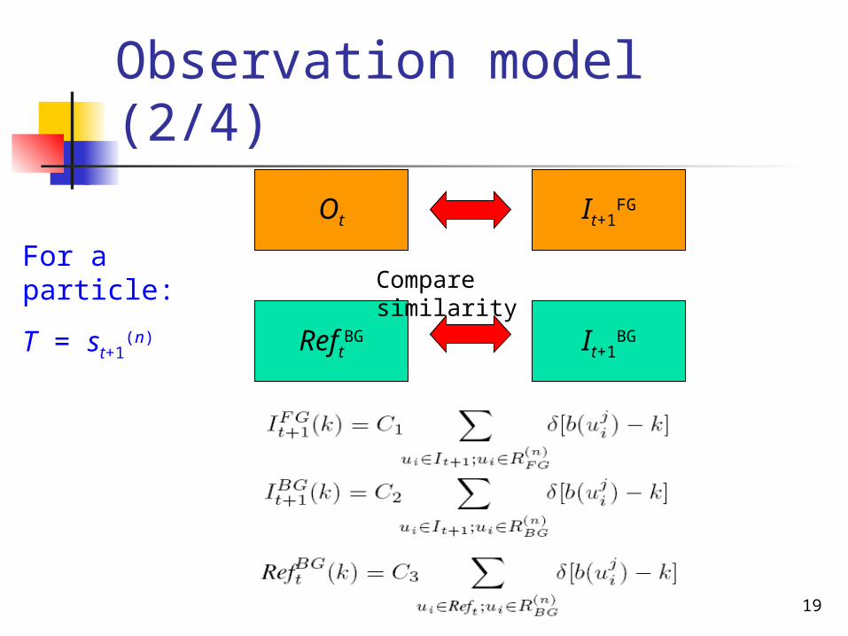
Observation model (2/4)

ReftBG It+1

BG

It+1FGOt

For a particle:

T = st+1(n)

Compare similarity

20

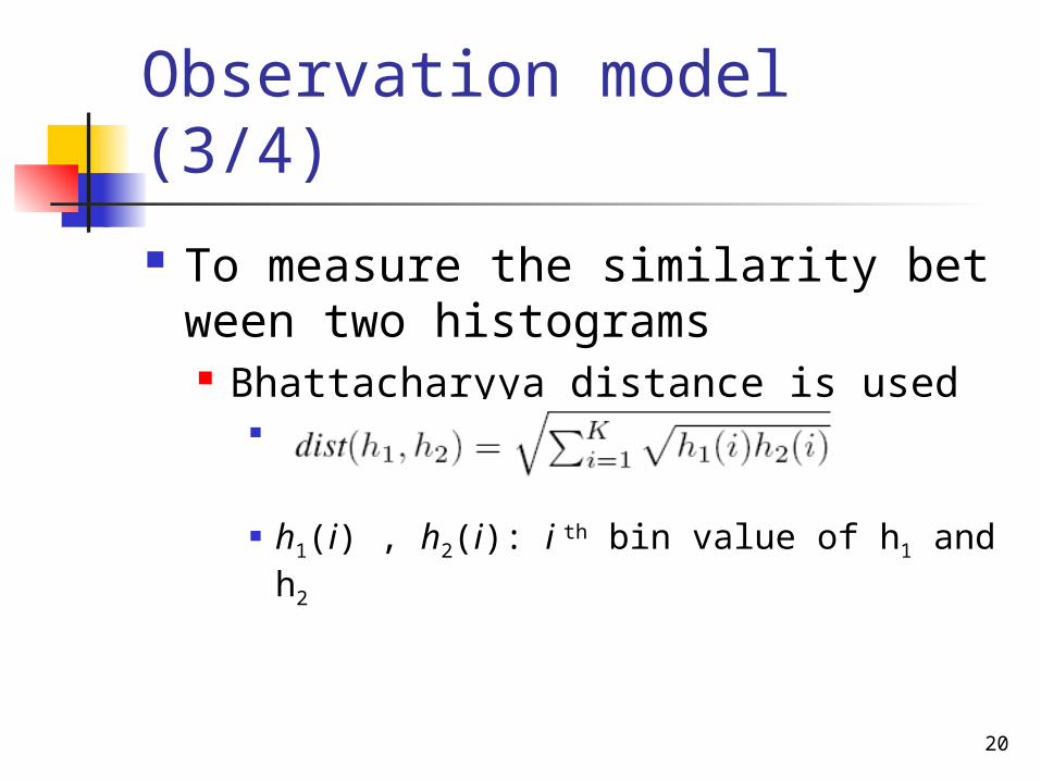
Observation model (3/4)

To measure the similarity between two histograms Bhattacharyya distance is used

h1(i) , h2(i): i th bin value of h1 and h2

21

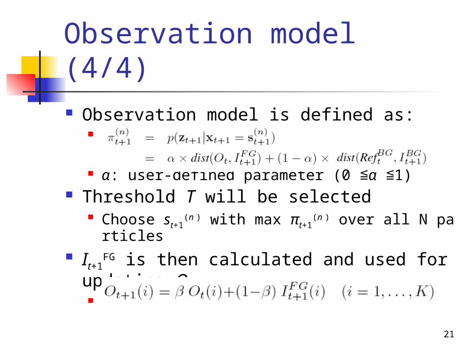
Observation model (4/4) Observation model is defined as:

α: user-defined parameter (0 ≦α ≦1) Threshold T will be selected

Choose st+1(n ) with max πt+1

(n ) over all N particles It+1

FG is then calculated and used for updating Ot

22

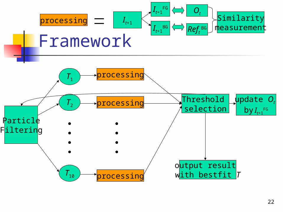
Framework

ParticleFiltering

T1

T2

T10

It+1

It+1FG

It+1BG

Ot

Reft BG

Similaritymeasurement

processing

processing

processing

Threshold selection

update Ot

by It+1FG

processing

output result with bestfit T

23

Outline

Introduction General BG Modeling Description Variable Threshold Selection Experiment results Conclusion

24

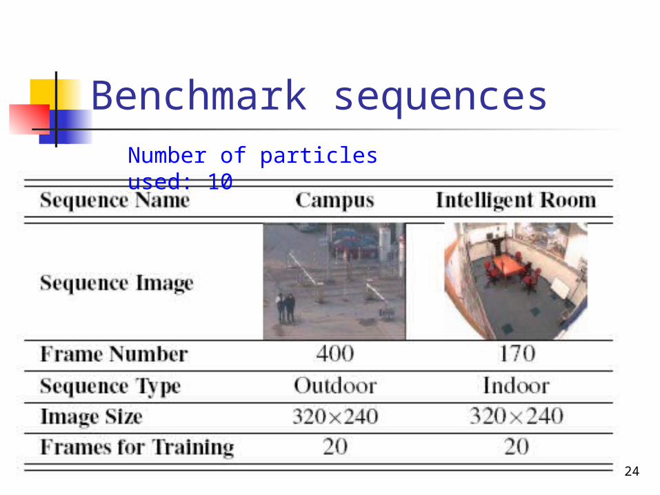
Benchmark sequencesNumber of particles used: 10

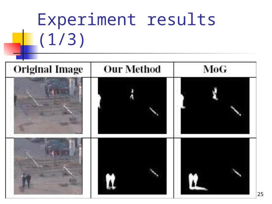
25

Experiment results (1/3)

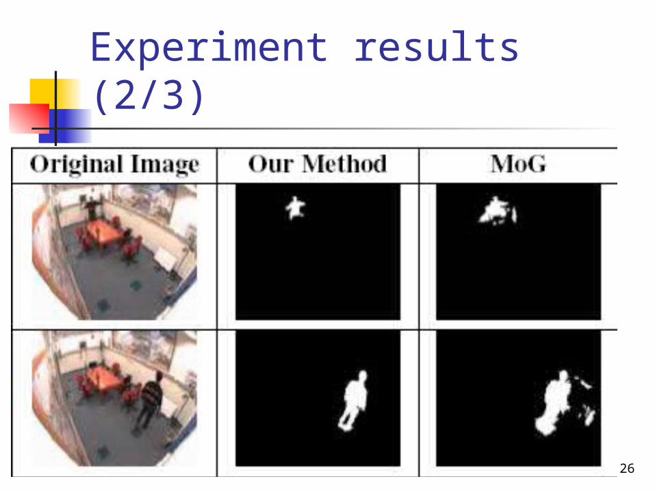
26

Experiment results (2/3)

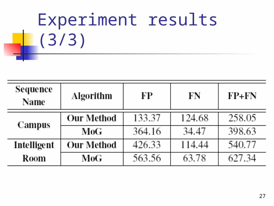
27

Experiment results (3/3)

28

Outline

Introduction General BG Modeling Description Variable Threshold Selection Experiment results Conclusion

29

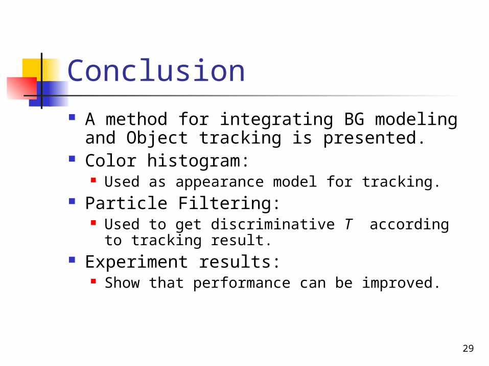
Conclusion A method for integrating BG modeling

and Object tracking is presented. Color histogram:

Used as appearance model for tracking. Particle Filtering:

Used to get discriminative T according to tracking result.

Experiment results: Show that performance can be improved.

30

Thank you Thanks for your listening.