Embed Size (px)
Citation preview

arX
iv:1
401.
4663
v2 [
cs.IT
] 25
Jul
201
41
Impact of Correlation between Nakagami-m
Interferers on Coverage Probability and Rate in
Cellular Systems
Suman Kumar Sheetal Kalyani
Dept. of Electrical Engineering
IIT Madras
Chennai 600036, India
{ee10d040,skalyani}@ee.iitm.ac.in
Abstract
Coverage probability and rate expressions are theoretically compared for the following cases:(i).
Both the user channel and theN interferers are independent and non identical Nakagami-m distributed
random variables (RVs).(ii). TheN interferers are correlated Nakagami-m RVs. It is analytically shown
that the coverage probability in the presence of correlatedinterferers is greater than or equal to the
coverage probability in the presence of non-identical independent interferers when the shape parameter
of the channel between the user and its base station is not greater than one. It is further analytically
shown that the average rate in the presence of correlated interferers is greater than or equal to the
average rate in the presence of non-identical independent interferers. Simulation results are provided
and these match with the obtained theoretical results. The utility of our results are also discussed.
Index Terms
Majorization theory, Stochastic ordering, Nakagami-m fading, Correlation, Coverage probability,
Average rate.
I. INTRODUCTION
Performance degradation of wireless communication is typically caused by multipath fading
and co-channel interference. Various fading models have been studied in literature for modeling

2
the interferers and user channels. Among them, the Nakagami-m distribution is a very popular
fading model, and Rayleigh fading can be treated as a specialcase of Nakagami-m fading [1].
Coverage probability1 is an important metric for performance evaluation of cellular systems
and for Nakagami-m fading environment it has been studied extensively for both independent
and correlated interferers case [2]–[10]. In the case wherethe fading parameters are arbitrary and
possibly non-identical for theN Nakagami-m interferers and the fading parameter for the user
channel is also arbitrary, coverage probability expression has been derived in terms of integral
in [9], infinite series in [5], [6], [8] and multiple series in[10].
Typically, in practical scenario correlation exists amongthe interferers [11]–[14]. For example
in cellular networks when two base stations (BSs) from adjacent sectors act as interferers, the
interferers are correlated and it is mandated that while performing system level simulation, this
correlation be explicitly introduced in the system [15]. Considering the impact of correlation in
the large scale shadowing component and the small scale multipath component is also an essential
step towards modeling the channel. The decorrelation distance in multipath components is lower
when compared to shadowing components since shadowing is related to terrain configuration
and/or large obstacles between transmitter and receiver [13].
For more general fading distributions, namely theη − µ fading [16] which also includes
Nakagami-m fading distribution as a special case, the coverage probability has been studied for
both independent and correlated interferers case [17]–[19]. In particular, Rayleigh fading for
interferers channel, andη − µ fading for the user channel are assumed in [17]. In [18],η − µ
fading has been considered assuming integer values of fading parameterµ for interferers channel
and arbitrary fading parameterµ for the user channel. Also,η − µ fading with integer values
of fading parameterµ for either the user channel or the interferer channel but notfor both are
assumed in [19].
However, to the best of our knowledge, no prior work in open literature has analytically
compared the coverage probability and rate when interferers are independent with the coverage
probability and rate when interferers are correlated. In this work, for Nakagami-m fading we
compare the coverage probability when the interferers are independent and non identically
1It is a probability that a user can achieve a target Signal-to-Interference-plus-noise-Ratio (SINR)T , and outage probability
is the complement of coverage probability.

3
distributed (i.n.i.d.) with the coverage probability whenthe interferers are positively correlated2
using majorization theory. It is analytically shown that the coverage probability in presence of
correlated interferers is higher than the coverage probability when the interferers are i.n.i.d.,
when the user channel’s shape parameter is lesser than or equal to one, and the interferers have
Nakagami-m fading with arbitrary parameters (i.e., shape parameter can be less than or greater
than one). We also show that when the user channel’s shape parameter is greater than one,
one cannot say whether coverage probability is higher or lower for the correlated case when
compared to the independent case, and in some cases coverageprobability is higher while in
other cases it is lower3.
We further analytically compare the average rate when the interferers are i.n.i.d. with the
average rate when the interferers are correlated using stochastic ordering theory. It is shown that
the average rate in the presence of positively correlated interferers is higher than the average
rate in the presence of i.n.i.d. interferers. Our results show that correlation among interferers is
beneficial for the desired user. We briefly discuss how the desired user can exploit this correlation
among the interferers to improve its rate in Section VI. We have also carried out extensive
simulations for both the i.n.i.d. interferers case and the correlated interferers case and some of
these results are reported in Section VI. In all the cases, the simulation results match with our
theoretical results. The work done here can be easily extended to the scenario where the user’s
channel experience Nakagami-m fading and interfering channel experienceη − µ fading with
half integer or integer value of parameterµ.
II. SYSTEM MODEL
We consider a homogeneous macrocell network with hexagonalstructure having inter cell site
distance2R as shown in Fig. 1. The Signal-to-Interference-Ratio (SIR)η of a user located atr
2If cov(Xi, Xj) ≥ 0 thenXi andXj are positively correlated RVs, wherecov(Xi, Xj) denotes the covariance betweenXi
andXj [20].
3The expression for outage probability given in [17]–[19] are in terms of multiple series. However, motivated by the bit error
probability expression in the multiple antenna system in the presence of generalized fading model [21]–[26], we have given
equivalent expressions for coverage probability in terms of Lauricella hypergeometric function, since that simplifies the analysis
required for comparison between i.n.i.d. and correlated interferers case significantly.

4
meters from the BS is given by
η(r) =Pgr−β
∑
i∈φ
Phid−βi
, (1)
whereφ denotes the set of interfering BSs andN = |φ| denotes the cardinality of the setφ.
The transmit power of a BS is denoted byP . A standard path loss modelr−β is considered,
whereβ ≥ 2 is the path loss exponent. Note that for the path loss modelr−β to be valid, it is
assumed that users are at least a minimum distanced meter away from the BS. An interference
limited network is assumed, and hence the noise power is neglected. The distance between user
to tagged BS (own BS) and theith interfering BS is denoted byr anddi, respectively. The user
channel’s power and the channel power betweenith interfering BS and user are gamma distributed
(corresponds to Nakagami-m fading) withg ∼ G(αu, λu) andhi ∼ G(αi, λi), respectively. The
pdf of the gamma RVg is given by
fY (y) =yαu−1e−
yλu
(λu)αuΓ(αu), y ≥ 0 (2)
where,αu ≥ 0.5 is the shape parameter,λu > 0 denotes the scale parameter, andΓ(.) denotes
the gamma function. The coverage probability of a user located at distancer meters from the
BS is defined as
Pc(T, r) = P (η(r) > T ) = P
(
gr−β
I> T
)
= P
(
I <gr−β
T
)
(3)
where T denotes the target SIR, andI =∑
i∈φ
hid−βi . Since hi ∼ G(αi, λi), henceI is the
sum of weighted i.n.i.d. gamma variates with weightsd−βi . We will use the fact that weighted
gamma variatesh′i = wihi can be written as gamma variates with weighted scale parameter i.e.,
h′i ∼ G(αi, λid
−βi ) [27]. Thus,I =
∑
i∈φ
h′i is the sum ofN i.n.i.d gamma variates. The pdf of the
sum of i.n.i.d. and correlated gamma RVs has been extensively studied in [6], [21], [28]–[34]
and references therein. In the context of this paper, we use the confluent Lauricella function
representation of the pdf of the sum of gamma variates.
The sum,X of N i.n.i.d. gamma RVs,h′i ∼ G(αi, λ
′i) whereλ′
i = λid−βi has a pdf given by
[21], [35], [36],
fX(x) =x
N∑
i=1
αi−1
N∏
i=1
(λ′i)αiΓ
(
N∑
i=1
αi
)φ(N)2
(
α1, · · · , αN ;
N∑
i=1
αi;−x
λ′1
, · · · , −x
λ′N
)
, x ≥ 0 (4)

5
whereφ(N)2 (.) is the confluent Lauricella function [35]–[37]. The cumulative distribution function
(cdf) of X is given by
FX(x) =x
N∑
i=1
αi
N∏
i=1
(λ′i)αiΓ
(
N∑
i=1
αi + 1
)φ(N)2
(
α1, · · · , αN ;N∑
i=1
αi + 1;−x
λ′1
, · · · , −x
λ′N
)
. (5)
0
6
13
4
5
2
9
15
7
1713
11
1812
16
10
14
8
2R
Fig. 1: Macrocell network with hexagonal tessellation having inter cell site distance2R
III. COVERAGE PROBABILITY
In this section, the coverage probability expression is given in terms of special functions for
both the i.n.i.d. interferers case and correlated interferers case.
A. Coverage Probability in Presence of i.n.i.d. Nakagami-m Fading
The coverage probability expression can be written asP(
I < gr−β
T
)
. Using the fact thatI is
the sum ofN i.n.i.d. gamma variates, one obtains,
Pc(T, r) = Eg
(
gr−β
T
)
N∑
i=1
αi
Γ
(
N∑
i=1
αi + 1
)
N∏
i=1
(λ′i)αi
φ(N)2
(
α1, · · · , αN ;N∑
i=1
αi + 1;−gr−β
Tλ′1
, · · · , −gr−β
Tλ′N
)
,
(6)
whereEg denotes expectation with respect to RVg which is gamma distributed. Using trans-
formation of variables withgλ= t, and the fact thatg ∼ G(αu, λu), (6) can be further simplified

6
as
Pc(T, r) = K ′λ
N∑
i=1
αi+αu
∞∫
0
t
N∑
i=1
αi+αu−1e−t
Γ
(
N∑
i=1
αi + αu
)φ(N)2
(
α1, · · ·αN ;N∑
i=1
αi + 1;−tλr−β
Tλ′1
, · · · −tλr−β
Tλ′N
)
dt.
(7)
where,K ′ = 1λαu
Γ
(
N∑
i=1
αi+αu
)
Γ
(
N∑
i=1
αi+1
)
1Γ(αu)
N∏
i=1
(
1λ′ir
βT
)αi
. In order to simplify (7), we use the following
integral equation [36, P. 286, Eq 43]
F(N)D [αu, β1, · · · , βN ; γ; x1, · · · , xN ] =
1
Γ(αu)
∞∫
0
e−ttαu−1φN2 [ β1, · · · , β2, γ; x1t, · · · , xN t]dt,
(8)
max{Re(x1), · · · , Re(xN)} < 1, Re(αu) > 0;
HereF (N)D [a, b1, · · · , bN ; c; x1, · · · , xN ] is the Lauricella’s function of the fourth kind [38]. Using
(8) to evaluate (7), one obtains
Pc(T, r) =Γ
(
N∑
i=1
αi+αu
)
Γ
(
N∑
i=1
αi+1
)
1Γ(αu)
N∏
i=1
(
λλ′ir
βT
)αi
F(N)D
[
N∑
i=1
αi + αu, α1, · · · , αN ;N∑
i=1
αi + 1; −λr−β
Tλ′1
, · · · , −λr−β
Tλ′N
]
,
(9)
F(N)D (.) can be evaluated by using single integral expression [21], [38] or multiple integral
expression [35]. A series expression forF(N)D (.) involving N-fold infinite sums is given by
F(N)D [a, b1, · · · , bN ; c; x1, · · · , xN ] =
∞∑
i1···iN=0
(a)i1+···+iN (b1)i1 · · · (bN )iN(c)i1+···+iN
xi11
i1!· · · x
iNN
iN !, (10)
max{|x1|, · · · |xN |} < 1,
where, (a)n denotes the Pochhammer symbol which is defined as(a)n = Γ(a+n)Γ(a)
. The series
expression for Lauricella’s function of the fourth kind converges ifmax{|x1|, · · · |xN |} < 1.
However from (9) it is apparent that convergence condition,i.e., maxi
|−λr−β
Tλ′i| < 1 is not always
satisfied, sincer < di. Hence in order to obtain a series expression forF(N)D (.) which converges,
we use the following property of the Lauricella’s function of the fourth kind [35, p.286].
F(N)D [a, b1, · · · , bN ; c; x1, · · · , xN ] =
[
∏Ni=1(1− xi)
−bi
]
F(N)D
(
c− a, b1, · · · , bN ; c; x1
x1−1, · · · , xN
xN−1
)
(11)
7
and rewrite (9) as
Pc(T, r) =Γ
(
N∑
i=1
αi+αu
)
Γ
(
N∑
i=1
αi+1
)
Γ(αu)
N∏
i=1
(
λλ+λ′
irβT
)αi
F(N)D
[
1− αu, α1, · · · , αN ;N∑
i=1
αi + 1; λλ+rβλ′
1T, · · · , λ
λ+rβλ′NT
]
(12)
B. Coverage Probability in Presence of Correlated Interferers
In this subsection, we obtain the coverage probability expression in presence of correlated
interferers, when the shape parameter of all the interferers are identical. The sum,Z of N
correlated not necessarily identically distributed gammaRVs Yi ∼ G(αc, λ′i) has a cumulative
distribution function given by [31], [32],
FZ(z) =zNαc
det(A)αcΓ (Nαc + 1)φ(N)2
(
αc, · · · , αc;Nαc + 1;−z
λ1
, · · · , −z
λN
)
,
here,A = DC, whereD is the diagonal matrix with entriesλ′i andC is the symmetric positive
definite (s.p.d.)N ×N matrix defined by
C =
1√ρ12 ...
√ρ1N
√ρ21 1 ...
√ρ2N
· · · · · · . . . · · ·√ρN1 · · · · · · 1
, (13)
whereρij denotes the correlation coefficient betweenYi andYj, and is given by,
ρij = ρji =cov(Yi, Yj)
√
var(Yi)var(Yj), 0 ≤ ρij ≤ 1, i, j = 1, 2, · · · , N. (14)
cov(Yi, Yj) andvar(Yi) denote the covariance betweenYi andYj and variance ofYi, respectively.
det(A) =N∏
i=1
λi is the determinant of the matrixA, and λis are the eigenvalues ofA. Note
that λi > 0 ∀i, sinceC is s.p.d. and the diagonal elements ofA are equal toλ′i. The functional
form of cdf of sum of correlated gamma RVs is similar to the cdfof sum of i.n.i.d. gamma
RVs. Hence the coverage probability in the presence of correlated interferersP cc (T, r) can be
similarly derived and one obtains
P cc (T, r) =
Γ(Nαc+αu)Γ(Nαc+1)
1Γ(αu)
N∏
i=1
(
λ
λ+λirβT
)αc
F(N)D
[
1− αu, αc, · · ·αc;Nαc + 1; λ
λ+rβ λ1T, · · · λ
λ+rβ λNT
]
,
(15)

8
However, note that here the coverage probability is a function of the eigenvalues ofA and
the shape parameter of the user and interferer channels while in the i.n.i.d. case it was only a
function of the shape parameters and scale parameters.
IV. COMPARISON OFCOVERAGE PROBABILITY
In this section, we compare the coverage probability in the i.n.i.d. case and correlated case,
and analytically quantify the impact of correlation. Note that the coverage probability expression
for the correlated case is derived when the interferers shape parameter are all equal and hence for
a fair comparison we consider equal shape parameter for the i.n.i.d. case also, i.e.,αi = αc ∀i.We first start with the special case when user channel’s fading is Rayleigh (i.e,αu = 1) and
interferers have Nakagami-m fading with arbitrary parameters. Whenαu = 1 andαi = αc ∀i,then the coverage probability in the i.n.i.d. case given in (12) reduces to
Pc(T, r) =
N∏
i=1
(
λ
λ+ λ′ir
βT
)αc
F(N)D
[
0, αc, · · · , αc;
N∑
i=1
αc + 1;λ
λ+ rβλ′1T
, · · · , λ
λ+ rβλ′NT
]
.
(16)
Using the fact that(0)0 = 1 and (0)k = 0 ∀ k ≥ 1, the coverage probability is now given by
Pc(T, r) =N∏
i=1
(
1
1 + λ′irβTλ
)αc
(17)
Similarly, the coverage probability in correlated caseP cc (T, r) is given by
P cc (T, r) =
N∏
i=1
(
1
1 + λirβTλ
)αc
. (18)
We now state and prove the following theorem for the case where the user channel undergoes
Rayleigh fading and interferers experience Nakagami-m fading and then generalize it to the case
where user also experiences Nakagami-m fading.
Theorem 1. The coverage probability in correlated case is higher than that of the i.n.i.d. case,
when user’s channel undergoes Rayleigh fading, i.e.,
N∏
i=1
(
1
1 + kλi
)αc
≥N∏
i=1
(
1
1 + kλ′i
)αc
(19)
where λis are the eigenvalues of matrix A and λ′is are the scale parameter for the i.n.i.d. case
and k = rβTλ
is a non negative constant.

9
Proof: Note that sinceA = DC, the diagonal elements ofA areλ′is. We will briefly state
two well known results from majorization theory4 which we will use to prove Theorem1.
Theorem 2. If H is an n×n Hermitian matrix with diagonal elements b1, · · · bn and eigenvalues
a1, · · ·an then
a ≻ b (21)
Proof: The details of the proof can be found in [39, P. 300, B.1.].
In our case, sinceλis are the eigenvalues andλ′is are the diagonal elements of a symmetric
matrix A hence from Theorem2, λ ≻ λ′ whereλ = [λ1, · · · , λn] andλ′ = [λ′1, · · · , λ′
n].
Proposition 1. If function φ is symmetric and convex, then φ is Schur-convex function. Conse-
quently, x ≻ y implies φ(x) ≥ φ(y).
Proof: For the details of this proof please refer to [39, P. 97, C.2.].
Now if it can be shown thatN∏
i=1
(
11+kλ′
i
)αc
(
andN∏
i=1
(
1
1+kλi
)αc
)
is a Schur-convex function
then by a simple application of Proposition1 it is evident thatN∏
i=1
(
1
1+kλi
)αc
≥N∏
i=1
(
11+kλ′
i
)αc
.
To prove thatN∏
i=1
(
11+kxi
)αc
is a Schur convex function we need to show that it is a symmetric
and convex function [39].
It is apparent that the functionN∏
i=1
(
11+kxi
)αc
is a symmetric function due to the fact that any
two of its arguments can be interchanged without changing the value of the function. So we
now need to show that the functionf(x1, · · · , xn) =N∏
i=1
(
11+kxi
)ai
is a convex function where
xi ≥ 0, ai > 0. The functionf(x1, · · · , xn) is convex if and only if its Hessian∇2 f is positive
4The notationa ≻ b indicate that vectorb is majorized by vectora. Let a = [a1, · · · an] and b = [b1, · · · bn] with
a1 ≤, · · · ,≤ an and b1 ≤, · · · ,≤ bn thena ≻ b if and only if
k∑
i=1
bi ≥
k∑
i=1
ai, k = 1, · · · , n− 1, andn∑
i=1
bi =
n∑
i=1
ai. (20)
10
semi-definite [40]. Now,∇2 f can be computed as
∇2 f = k2N∏
i=1
(
1
1 + kxi
)ai
a1(a1+1)(1+kx1)2
a1a2(1+kx1)(1+kx2)
· · · a1an(1+kx1)(1+kxn)
a1a2(1+kx1)(1+kx2)
a2(a2+1)(1+kx2)2
· · · a2an(1+kx2)(1+kxn)
· · · · · · . . . · · ·a1an
(1+kx1)(1+kxn)a2an
(1+kx2)(1+kxn)· · · an(an+1)
(1+kxn)2
(22)
We now need to show that∇2 f is a positive semi-definite matrix. For a real symmetric matrix
M , if xTMx > 0 for everyN×1 nonzero real vectorx, then the matrixM is positive definite
(p.d.) matrix [41, P. 566]. We now rewrite the Hessian matrixas sum of two matrices and it is
then given by
∇2 f = k2N∏
i=1
(
1
1 + kxi
)ai
[P+Q]. (23)
Here,
P =
a21
(1+kx1)2a1a2
(1+kx1)(1+kx2)· · · a1an
(1+kx1)(1+kxn)
a1a2(1+kx1)(1+kx2)
a22(1+kx2)2
· · · a2an(1+kx2)(1+kxn)
· · · · · · . . . · · ·a1an
(1+kx1)(1+kxn)a2an
(1+kx2)(1+kxn)· · · a2n
(1+kxn)2
(24)
and
Q =
a1(1+kx1)2
0 · · · 0
0 a2(1+kx2)2
· · · 0
· · · · · · . . . · · ·0 0 · · · an
(1+kxn)2
. (25)
Here by definitionk2N∏
i=1
(
11+kxi
)ai
> 0. If now bothP andQ are p.d. then∇2 f is p.d. Note
that P can be written asUTU whereU =[
a1(1+kx1)
, a2(1+kx2)
, · · · , an(1+kxn)
]
is a N × 1 vector.
Hence,xTPx = xT (UTU)x = ||Ux||2 > 0 for everyN × 1 nonzero real vectorx. Thus,P
is a p.d matrix. SinceQ is a diagonal matrix with positive entries,Q is also a p.d matrix. Since
sum of two p.d. matrix is p.d. matrix henceP +Q is a p.d. matrix. Thus,∇2 f is a p.d. matrix
andf(x1, · · · , xn) =N∏
i=1
(
11+kxi
)ai
is a convex function.
SinceN∏
i=1
(
11+kxi
)αc
is a convex function and a symmetric function therefore, it is a Schur-
convex function. We have shown thatλ ≻ λ′ andN∏
i=1
(
11+kxi
)αc
is a Schur-convex function.

11
Therefore, from Proposition 1,N∏
i=1
(
1
1+kλi
)αc
≥N∏
i=1
(
11+kλ′
i
)αc
.
Thus, the coverage probability in the presence of correlation among the interferers is greater
than or equal to the coverage probability in the i.n.i.d. case, when user channel undergoes
Rayleigh fading and the interferers shape parameterαi = αc ∀i. Now, we compare the coverage
probability for general case, i.e., whenαu is arbitrary.
Theorem 3. The coverage probability in the presence of the correlated interferers is greater
than or equal to the coverage probability in presence of i.n.i.d. interferers, when user channel’s
shape parameter is less than or equal to 1, i.e., αu ≤ 1. When αu > 1, coverage probability
in the presence of i.n.i.d. is not always lesser than the coverage probability in the presence of
correlated interferers.
Proof: Please see Appendix.
Summarizing, the coverage probability in the presence of correlated interferers is greater than
or equal to the coverage probability in presence of independent interferers, when user channel’s
shape parameter is less than or equal to1, i.e.,αu ≤ 1. Whenαu > 1, one can not say whether
coverage probability is better in correlated interferer case or independent interferer case. Note
that whenαu ≤ 1, usually the interferersαi is also smaller than1. However, the proof we have
holds for bothαi > 1 andαi < 1.
V. COMPARISON OFRATE
In this section, we compare the average rate when interferers are i.n.i.d with the average rate
when the interferers are correlated. We first start with the special case, whereαu ≤ 1, while
the interferer’s shape parameter is arbitrary. Then, the general case is analysed, i.e., when user’s
shape parameter and interferers shape parameter both can bearbitrary, and the scale parameters
are also arbitrary.
A. When user’s shape parameter is less than or equal to 1.
The average rate of a user at a distancer is R(r) = E[ln(1 + η(r))]. Using the fact that for
a positive RVX, E[X ] =∫
t>0
P (X > T )dt, one obtains
R(r) =
∫
t>0
P [ln(1 + η(r)) > t]dt. (26)

12
R(r)(a)=
∫
t>0
P [η(r) > et − 1]dt. (27)
Here (a) follows from the fact thatln(1 + η(r)) is a monotonic increasing function forη(r).
Similarly, for correlated case, average rate at distancer, R(r) is given by
R(r) =
∫
t>0
P [η(r) > et − 1]dt. (28)
Here η(r) denotes the SIR experienced by the user when interferers arecorrelated. Now, we
compareR(r) and R(r) whenαu ≤ 1 to see the impact of correlation on the average rate. The
integrands of (27) and (28), i.e.,P [η(r) > et − 1] andP [η(r) > et − 1] are equivalent to the
coverage probability expressions for independent interferers case and for correlated interferers
case evaluated atT = et − 1, respectively. It has been shown in Theorem3 that the coverage
probability in the presence of the correlated interferers is greater than or equal to the coverage
probability in the presence of independent interferers, when αu ≤ 1. In other words,P [η(r) >
et − 1] ≥ P [η(r) > et − 1], ∀ t whenαu ≤ 1. Therefore, it is apparent from (27) and (28) that
R(r) > R(r), whenαu ≤ 1 since for both integration is over the same interval.
Now, we will compare the average rate when bothαu andαi = αc ∀i are arbitrary. It is difficult
to compare the rate using the approach given above forαu ≤ 1 since coverage probability in
the presence of the correlated interferers can be greater orlower to the coverage probability in
the presence of independent interferers, whenαu > 1 (See Appendix for more detail). Hence
we compare the average rate using stochastic ordering theory.
B. When both user’s shape parameter and interferer’s shape parameter are arbitrary
In this subsection, we compareR = E[ln(1 + SI)], andR = E[ln(1 + S
I)] for arbitrary values
of shape parameter. Hereη(r) = SI
and η(r) = S
I, whereS is the desired user channel power.
Using iterated expectation one can rewrite the rates as
R = ES
[
EI
[
ln
(
1 +S
I
)∣
∣
∣
∣
S = s
]]
, and R = ES
[
EI
[
ln
(
1 +S
I
)∣
∣
∣
∣
S = s
]]
. (29)
Since the expectation operator preserves inequalities, therefore if we can show thatEI
[
ln
(
1+
S
I
)∣
∣
∣
∣
S = s
]
≥ EI
[
ln(
1 + SI
)
∣
∣
∣
∣
S = s
]
, then this impliesR ≥ R.

13
HereI and I are the sum of independent and correlated interferers, respectively. The sum of
interference power in the i.n.i.d. case can be written as
I =
N∑
i=1
h′i =
N∑
i=1
λ′iGi with h′
i ∼ G(αc, λ′i) andGi ∼ G(αc, 1) (30)
Similarly, for the correlated case,
I =
N∑
i=1
hi =
N∑
i=1
λiGi, (31)
where hi ∼ G(αc, λ′i). Recall that thesehi are correlated with the correlation structure defined
by correlation matrixC given in (13), andλis are the eigenvalues of the matrixA = DC. In
other words one can obtain a correlated sum of gamma variatesby multiplying independent and
identical distributed (i.i.d.) gamma variates with weightλis. We now briefly state the theorems
in stochastic order theory that we will use to show thatR is always greater than equal toR.
Theorem 4. Let X1, X2, · · · , XN be exchangeable RVs. Let a = (a1, a2, · · · , aN) and b =
(b1, b2, · · · , bN) be two vectors of constants. If a ≺ b, then
N∑
i=1
aiXi ≤cx
N∑
i=1
biXi. (32)
Proof: The details of the proof is given in [42, Theorem 3.A.35].
Here the notationX ≤cx Y denote thatX is smaller thanY in convex order5. Also, note that
a sequence of RVsX1, · · ·XN is said to be exchangeable if for allN andπ ∈ S(N) it holds
that X1 · · ·XND= Xπ(1) · · ·Xπ(N) whereS(N) is the group of permutations of{1, · · ·N} and
D= denotes equality in distribution [43]. Furthermore, ifXis are identically distributed, they are
exchangeable [42, P. 129]. HenceGis are exchangeable since they are identically distributed.It
has already been shown thatλ ≻ λ′ in Section IV. Hence by a direct application of Theorem
4, one obtains,I ≤cx I.
Theorem 5. If X ≤cx Y and f(.) is convex, then E[f(X)] ≤ E[f(Y )].
Proof: The details of the proof is given in [44, Theorem 7.6.2].
5If X andY are two RVs such thatE[φ(X)] ≤ E[φ(Y )] for all convex functionφ : R → R, provided the expectation exist.
ThenX is said to be smaller thanY in the convex order.

14
ln(1+ kx) is a convex function whenk ≥ 0 andx ≥ 0 due to the fact that double differentiation
of ln(1 + kx) is always non negative, i.e.,
∂∂ ln( k
x+1)∂x
∂x= k(k+2x)
x2(k+x)2≥ 0. Note thatS and I are non
negative RVs, hence by a direct application of Theorem5, one obtains
EI
[
ln
(
1 +S
I
)∣
∣
∣
∣
S = s
]
≥ EI
[
ln
(
1 +S
I
)∣
∣
∣
∣
S = s
]
(33)
Since expectation preserve inequalities therefore,ES[EI [ln(1 + SI)]] ≤ ES[EI [ln(1 + S
I)]]. In
other words, positive correlation among the interferers increases the average rate.
Summarizing, the average rate in the presence of the positive correlated interferers is always
greater than or equal to the average rate in the presence of independent interferers. Now we
briefly discuss the utility of our results in the presence of log normal fading.
C. Log Normal Shadowing
Although all the analysis so far (comparison of the coverageprobability and average rate)
considered only small scale fading and path loss, the analysis can be further extended to take
into account shadowing effects. In general, the large scalefading, i.e, log normal shadowing is
modeled by zero-mean log-normal distribution which is given by,
fX(x) =1
x√
2π( σdB
8.686)2
exp
(
− ln2(x)
2( σdB
8.686)2
)
, x > 0,
whereσdB is the shadow standard deviation represented in dB. Typically the value ofσdB varies
from 3 dB to 10 dB [15], [45]. It is shown in [46] that the pdf of the compositefading channel
(fading and shadowing) can be expressed using the generalized-K (Gamma-Gamma) model. Also
in [47], it has been shown that the generalized-K pdf can be well approximated by Gamma pdf
G(αl, λl) using the moment matching method, withαl andλl are given by
αl =1
( 1αu
+ 1) exp(( σdB
8.686)2)− 1
=αu
(αu + 1) exp(( σdB
8.686)2)− αu
(34)
andλl = (1 + αu)λu exp
(
3( σdB
8.686)2
2
)
− αuλu exp
(
( σdB
8.686)2
2
)
(35)
Thus, SIRηl of a user can now given by
ηl(r) =Pglr
−β
∑
i∈φ
Phlid
−βi
(36)
15
where gl ∼ G(αl, λl) and hli ∼ G(αl
i, λli). Here αl
i = 1( 1
αi+1) exp((
σdB8.686
)2)−1and λl
i = (1 +
αi)λi exp(
3(σdB8.686
)2
2
)
− αiλi exp(
(σdB8.686
)2
2
)
. One can now derive the coverage probability expres-
sion in the presence of log-normal shadowingP lc(T, r) using the methods in Section II to obtain,
P lc(T, r) =
Γ
(
N∑
i=1
αli+αl
)
Γ
(
N∑
i=1
αli+1
)
Γ(αl)
N∏
i=1
(
λl
λl+λlid
−βi rβT
)αli ×
F(N)D
[
1− αl, αl1, · · · , αl
N ;N∑
i=1
αli + 1; λl
λl+rβλl1d−β1
T, · · · , λl
λl+rβλlNd−βN
T
]
(37)
Further, the correlation coefficient between two identically distributed generalized-K RVs is
derived in [48, Lemma 1], and it is in terms of correlation coefficient of the RVs corresponding
to the short term fading component (ρi,j) and the correlation coefficient of the RVs corresponding
to the shadowing component(ρsi,j). The resultant correlation coefficient (ρli,j) is then given by
ρli,j =
ρi,j
(exp( σdB8.686
)2)−1)+ ρsi,jαc + ρi,jρ
si,j
αc +1
(exp( σdB8.686
)2)−1)+ 1
(38)
Now, similar to the independent case, the coverage probability for correlated interferers case
Pc
l(T, r) is given by given by
Pc
l(T, r) =
Γ(Nαlc+αl)
Γ(Nαlc+1)Γ(αl)
N∏
i=1
(
λl
λl+λlir
βT
)αli × (39)
F(N)D
[
1− αl, αlc, · · · , αl
c;Nαlc + 1; λl
λl+rβ λl1T, · · · , λl
λl+rβ λlNT
]
(40)
whereλlis are the eigenvalues ofAl = DlCl, whereDl is the diagonal matrix with entriesλl
id−βi
andCl is defined by
Cl =
1√
ρl12 ...√
ρl1N√
ρl21 1 ...√
ρl2N
· · · · · · . . . · · ·√
ρlN1 · · · · · · 1
, (41)
with ρlij is given by (38). Note that both (37) and (40) have a similar functional form and they
both are also similar to (12) and (15), respectively. Hence now the coverage probability and
average rate for the i.n.i.d. case and correlated case can becompared using the methods outlined
in Section IV and Section V. In other words, it can be shown that the coverage probability in the
presence of correlated interferers is greater than or equalto the coverage probability in presence

16
of independent interferers, when user’s shape parameter isless than or equal to1, i.e.,αl ≤ 1,
in the presence of shadow fading. Also, the average rate in the presence of positive correlated
interferers is always greater than or equal to the average rate in the presence of independent
interferers, in the presence of shadow fading.
D. Extension of this work for η − µ fading
Recently, theη−µ fading distribution with two shape parametersη andµ has been proposed
to model a general non-line-of-sight propagation scenario[16]. It includes Nakagami-q (Hoyt),
one sided Gaussian, Rayleigh and Nakagami-m as special cases. It has been shown in [49] that
the sum of correlatedη−µ power RVs with half integer or integer value of parameterµ can be
represented by the sum of independent gamma RVs with suitable parameters. Hence, our analysis
on the impact of correlation on the coverage probability andaverage rate can be extended to
the scenarios where the user’s channel experience Nakagami-m fading and interfering channel
experienceη − µ fading with half integer or integer value of parameterµ. Although, there is
a restriction on the parameterµ, it still entitles us to include one-sided Gaussian, Rayleigh,
Nakagami-q (Hoyt) and Nakagami-m (with integer m) fading for the interfering signal in our
analysis.
In the next section, we will show simulation results and discuss how those match with the
theoretical results. We also briefly discuss how the analysis carried out in this work can be of
utility to the network and the user.
VI. NUMERICAL ANALYSIS AND APPLICATION
In this section, we give some simulation results for the coverage probability and rate for both
independent and correlated case. The impact of correlationamong interferers on the coverage
probability and rate is discussed and it is observed that in all simulations the rate is higher for the
correlated case when compared to i.n.i.d. case. For the simulations, we consider a19 cell system
with hexagonal structure having inter cell site distance2R = 1732 meters as shown in Fig. 1.
For each user which is connected to the0th cell we generate the gamma RV corresponding to its
own channel and gamma RVs corresponding to the18 interferers and then compute SIR. Then,
using the simulated SIR, the coverage probability and average rate can be obtained and they are
averaged over 10000 times.

17
400 500 600 700 800 900
0.1
0.2
0.3
0.4
0.5
0.6
0.7
0.8
0.9
1β = 4, T = 3 dB, λ = 1, λi = 2
Distance from Base station (m)
Cov
erag
e P
roba
bilit
y
Analytical α=1.5, αi=1
Simulation α=1.5, αi=1
Analytical α=2.5, αi=1
Simulation α=2.5, αi=1
Analytical α=2.5, αi=1.5
Simulation α=2.5, αi=1.5
Fig. 2: Coverage Probability of a user with respect to distance from the BS in presence of
Nakagami-m fading
Fig. 2 shows the impact of shape parameter on the coverage probability in the i.n.i.d. case. We
first note that the simulation results exactly match with theanalytical results (computed using
Eq. (12) ). Secondly, it can be observed that as user channel’s shape parameter(αu) increases
while keeping the interferer shape parameters fixed, the coverage probability increases. Whereas,
when interferer channel’s shape parameter increases and the user channel’s shape parameter is
fixed, the coverage probability decreases as expected.
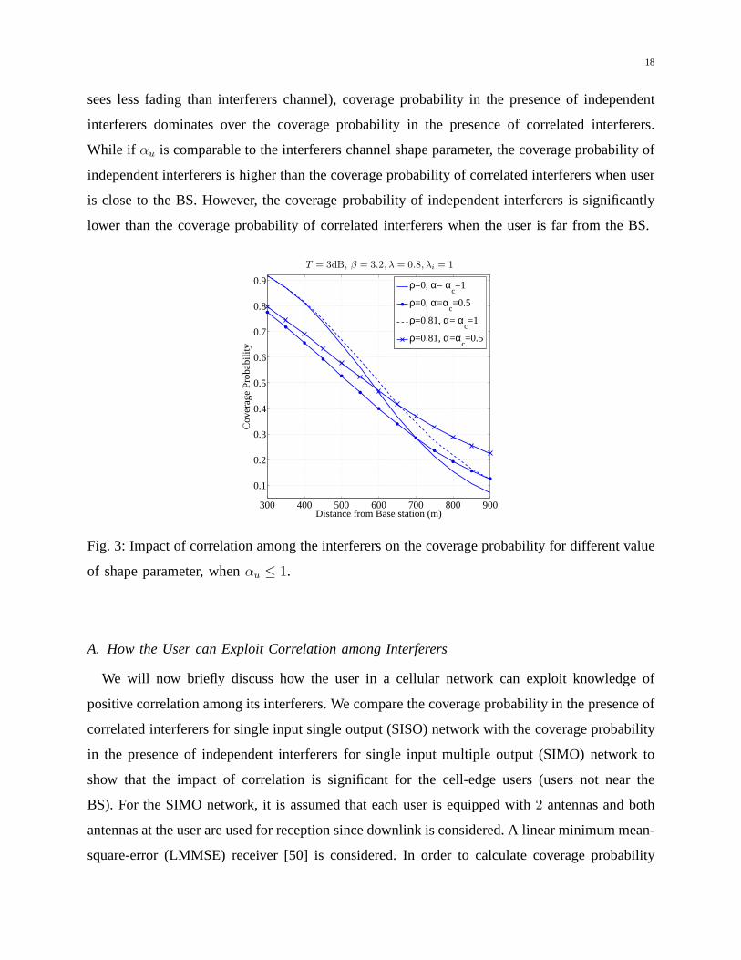
Fig. 3 and Fig. 4 depict the impact of correlation among the interferers on the coverage
probability for different values of shape parameter. The correlation among the interferers is
defined by the correlation matrix in (13) withρpq = ρ|p−q| wherep, q = 1, · · · , N [33]. From
Fig. 3, it can be observed that forαu = 0.5 andαu = 1, coverage probability in presence of
correlation is higher than that of independent scenario (which match our analytical result). For
example, atαu = 0.5, coverage probability increases from0.12 in the i.n.i.d case to0.22 in the
correlated case and atαu = 1, coverage probability increases from0.07 to 0.12 when user is at
distance900m from the BS. In Fig. 4, whereαu > 1, one cannot say that coverage probability in
presence of correlation is higher or lower than that of independent scenario. However, it can be
seen that whenαu is significantly higher than the interferers shape parameter (i.e., user channel
18
sees less fading than interferers channel), coverage probability in the presence of independent
interferers dominates over the coverage probability in thepresence of correlated interferers.
While if αu is comparable to the interferers channel shape parameter, the coverage probability of
independent interferers is higher than the coverage probability of correlated interferers when user
is close to the BS. However, the coverage probability of independent interferers is significantly
lower than the coverage probability of correlated interferers when the user is far from the BS.
300 400 500 600 700 800 900
0.1
0.2
0.3
0.4
0.5
0.6
0.7
0.8
0.9
T = 3dB, β = 3.2, λ = 0.8, λi = 1
Distance from Base station (m)
Cov
erag
e P
roba
bilit
y
ρ=0, α= α
c=1
ρ=0, α=αc=0.5
ρ=0.81, α= αc=1
ρ=0.81, α=αc=0.5
Fig. 3: Impact of correlation among the interferers on the coverage probability for different value
of shape parameter, whenαu ≤ 1.
A. How the User can Exploit Correlation among Interferers
We will now briefly discuss how the user in a cellular network can exploit knowledge of
positive correlation among its interferers. We compare thecoverage probability in the presence of
correlated interferers for single input single output (SISO) network with the coverage probability
in the presence of independent interferers for single inputmultiple output (SIMO) network to
show that the impact of correlation is significant for the cell-edge users (users not near the
BS). For the SIMO network, it is assumed that each user is equipped with2 antennas and both
antennas at the user are used for reception since downlink isconsidered. A linear minimum mean-
square-error (LMMSE) receiver [50] is considered. In orderto calculate coverage probability

19
300 400 500 600 700 800 9000
0.1
0.2
0.3
0.4
0.5
0.6
0.7
0.8
0.9
1T = 3dB, β = 3.2, λ = 0.8, λi = 1
Distance from Base station (m)
Cov
erag
e P
roba
bilit
y
ρ=0, α=5, αc=1
ρ=0.81, α=5, αc=1
ρ=0, α=2, αc=1
ρ=0.81, α=2, αc=1
ρ=0, α=1.5, αc=1
ρ=0.81, α=1.5, αc=1
ρ=0, α=αc=5
ρ=0.81, α=αc=5
Fig. 4: Impact of correlation among the interferers on the coverage probability for different value
of shape parameter, whenαu > 1.
with a LMMSE receiver, it is assumed that the closest interferer can be completely cancelled
at the SIMO receiver. Fig. 5 plots the SISO coverage probability in the presence of correlated
interferers case and the coverage probability in the presence of i.n.i.d. interferers for a SIMO
network. It can be seen that forρ = 0.98, the SISO coverage probability for the correlated case6
is higher than the SIMO coverage probability for i.n.i.d. case. However, forρ = 0.81, SISO
coverage probability is close to the SIMO coverage probability at the cell-edge. For example,
the coverage probabilities forρ = 0.98, ρ = 0.81 and the SIMO case with i.n.i.d. interferers are
0.256, 0.2 and 0.18, respectively, when user is at distance900m from the BS. In other words,
correlation among the interferers seems to be as good as having one additional antenna at the
receiver capable of cancelling the dominant interferer.
Fig. 6 shows the average rate in the presence of correlation among the interferers and the
average rate in the presence of independent interferers forSISO case. It can be observed that
average rate is higher in the presence of correlated interferers. It can be also seen that for
6The correlation among the interferers is defined by the correlation matrix in (13) withρpq = ρ|p−q| wherep, q = 1, · · · , N

20
600 650 700 750 800 850 9000.05
0.1
0.15
0.2
0.25
0.3
0.35
0.4
0.45
0.5T = 3dB, β = 2.8, λ = λi = 1
Distance from the BS (m)
Cov
erag
e P
roba
bilit
y
Correlation, ρ = 0.98Independent, SIMOCorrelation, ρ = 0.81Correlation, ρ = 0.5Independent
Fig. 5: Comparison of coverage probability of correlated interferers with the coverage probability
of SIMO network. Hereαu = αi = 1.
ρ = 0.98, average rate for the correlated case is higher than that of the 1 × 2 SIMO network.
For example, average rates forρ = 0.98, the SIMO case and independent case are1.41 nats/Hz,
1.28 nats/Hz and1.09 nats/Hz, respectively, when user is at distance600m from the BS.
Fig. 7 presents the comparison of average rate in the presence of log normal shadowing. It can
be seen that for bothρ = 0.98 andρ = 0.81, the average rate of the correlated case is higher than
that of the1×2 SIMO network withρ = 0. In other words, in presence of shadowing the impact
of correlation is even more significant. For example, average rates for SISO case withρ = 0.98,
the SIMO case withρ = 0, and the SISO case withρ = 0 are 1.25 nats/Hz,0.86 nats/Hz and
0.71 nats/Hz, respectively when the user is at distance700m from the BS. Obviously, if one had
correlated interferers in the SIMO system that would again lead to improved coverage probability
and average rate and may be compared to a SIMO system with higher number of antennas. In
all three cases, it is apparent that if the correlation amongthe interferers is exploited, it leads
to performance results for a SISO system which are comparable to the performance of a1× 2
SIMO system with independent interferers.
We would also likely to briefly point out that the impact of correlation among the interferers
is like that of introducing interference alignment in a system. Interference alignment actually

21
300 400 500 600 700 800 900
0.5
1
1.5
2
2.5
3
α = αi = 1, λ = λi = 1, β = 3
Distance from the BS (meters)
Ave
rage
Rat
e (n
ats/
Hz)
Correlated, ρ = 0.98
SIMO, Independent
Correlated, ρ = 0.81
Independent
Fig. 6: Comparison of the average rate in presence of independent interferers with the average
rate in presence of correlated interferers.
300 400 500 600 700 800 9000
0.5
1
1.5
2
2.5
3
3.5α = αi = 1, λ = λi = 1, β = 3, σdB = 5dB
Distance from the BS (meters)
Ave
rage
Rat
e (n
ats/
Hz)
Correlated, ρ = ρs = 0.98
Correlated, ρ = ρs = 0.81
SIMO Independent
Correlated, ρ = ρs = 0.5
Independent
Fig. 7: Comparison of the average rate in the presence of log normal shadowing.
aligns interference using appropriate precoding so as reduce the number of interferers one needs
to cancel. Here the physical nature of the wireless channel and the presence of co-located
interferers also “aligns” the interferer partially. This is the reason one can get a gain equivalent

22
to 1× 2 system in a1× 1 system with correlated interferers provided the user knowsabout the
correlation.
Summarizing, our work is able to analytically shows the impact of correlated interferers on
coverage probability and rate. This can be used by the network and user to decide whether
one wants to use the antennas at the receiver for diversity gain or interference cancellation
depending on the information available about interferers correlation. Note that interferers from
adjacent sector of a BS will definitely be correlated [11]–[15]. We believe that this correlation
should be exploited, since the analysis shows that knowledge of correlation will lead to higher
coverage probability and rate.
VII. CONCLUSIONS
In this work, the coverage probability expressions and rateexpressions have been compared
analytically for following two cases:(a) Interferers and user channel having arbitrary Nakagami-
m fading parameters.(b) Interferers being correlated where the correlation is specified by a
correlation matrix. We have shown that the coverage probability in correlated interferer case
is higher than that of the independent case, when the user channel’s shape parameter is lesser
than or equal to one, and the interferers have Nakagami-m fading with arbitrary parameters.
Further, it has been shown that positive correlation among the interferers always increases the
average rate. We have also taken into account the shadow fading component in our analysis.
The impact of correlation seems even more pronounced in the presence of shadow fading. Our
results indicate that if the user is aware of the interfererscorrelation matrix then it can exploit
it since the correlated interferers behave like partially aligned interferers. This means that if the
user is aware of the correlation then one can obtain a rate equivalent to a1×2 system in a1×1
system depending on the correlation matrix structure. Extensive simulations were performed and
these match with the theoretical results.
APPENDIX
PROOF OFTHEOREM 3
The coverage probability expressions for the scenario wheninterferers are i.n.i.d. and the
scenario when interferers are correlated are given in (12) and (15), respectively and rewriting

23
them for the case whenαi = αc ∀i, one obtains
Pc(T, r) = K ′F(N)D
[
1− αu, αc, · · · , αc;Nαc + 1;λ
λ+ rβλ′1T
, · · · , λ
λ+ rβλ′NT
]
(42)
P cc (T, r) = KF
(N)D
[
1− αu, αc, · · · , αc;Nαc + 1;λ
λ+ rβλ1T, · · · , λ
λ+ rβλNT
]
, (43)
whereK ′ = Γ(Nαc+αu)Γ(Nαc+1)
1Γ(αu)
N∏
i=1
(
1
1+λ′irβTλ
)αc
and K = Γ(Nαc+αu)Γ(Nαc+1)
1Γ(αu)
N∏
i=1
(
1
1+λirβTλ
)αc
. From
Theorem1 it is clear thatK > K ′ . Now, we need to compare the Lauricella’s function of the
fourth kind of (42) and (43). Here, for comparison we use the series expression forFD(.).
We expand the series expression for the Lauricella’s function of the fourth kind in the following
form:
F(N)D [a, b, · · · , b; c; x1, · · · , xN ] =1 +K1,1
N∑
i=1
xi +K2,1
N∑
i=1
x2i +K2,2
∑
1≤i<j≤N
xixj +K3,1
N∑
i=1
x3i
+K3,2
N∑
i,j=1,s.t.i 6=j
x2ixj +K3,3
∑
1≤i<j<k≤N
xixjxk + · · · (44)
whereK1,1 = (a)1(b)1(c)11!
, K2,1 = (a)2(b)2(c)22!
, K2,2 = (a)2(b)1(b)1(c)21!1!
, K3,1 = (a)3(b)3(c)33!
, K3,2 = (a)3(b)2(b)1(c)32!1!
,
K3,3 =(a)3(b)1(b)1(b)1
(c)31!1!1!and so on.
Hence the coverage probability for independent case given in (42) can be written as
Pc(T, r) =K ′
[
1 +K1,1
N∑
i=1
(
1
1 + λ′irβTλ
)
+K2,1
N∑
i=1
(
1
1 + λ′irβTλ
)2
+K3,1
N∑
i=1
(
1
1 + λ′irβTλ
)3
+
K2,2
∑
1≤i<j≤N
(
1
1 + λ′irβTλ
)(
1
1 + λ′jrβTλ
)
+K3,2
N∑
i,j=1,s.t.i 6=j
(
1
1 + λ′irβTλ
)2(
1
1 + λ′jrβTλ
)
+
K3,3
∑
1≤i<j<k≤N
(
1
1 + λ′irβTλ
)(
1
1 + λ′jrβTλ
)(
1
1 + λ′krβTλ
)
+ · · ·]
(45)
Similarly, for the correlated case the coverage probability given in (43) can be written as
P cc (T, r) =K
[
1 +K1,1
N∑
i=1
(
1
1 + λirβTλ
)
+K2,1
N∑
i=1
(
1
1 + λirβTλ
)2
+K3,1
N∑
i=1
(
1
1 + λirβTλ
)3
+
K2,2
∑
1≤i<j≤N
(
1
1 + λirβTλ
)(
1
1 + λjrβTλ
)
+K3,2
N∑
i,j=1,s.t.i 6=j
(
1
1 + λirβTλ
)2(
1
1 + λjrβTλ
)
+
K3,3
∑
1≤i<j<k≤N
(
1
1 + λirβTλ
)(
1
1 + λjrβTλ
)(
1
1 + λkrβTλ
)
+ · · ·]
(46)

24
Here K1,1 = (1−αu)1(αc)1(Nαc+1)11!
, K2,1 = (1−αu)2(αc)2(Nαc+1)22!
, K2,2 = (1−αu)2(αc)1(αc)1(Nαc+1)21!1!
, K3,1 = (1−αu)3(αc)3(Nαc+1)33!
,
K3,2 =(1−αu)3(αc)2(αc)1
(Nαc+1)32!1!, K3,3 =
(1−αu)3(αc)1(αc)1(αc)1(Nαc+1)31!1!1!
and so on. Note that hereKi,j are the same
for both Pc(T, r) andP cc (T, r). Now, we want to show that each summation term in the series
expression is a Schur-convex function.
Each summation term in the series expression is symmetricaldue to the fact that any two of
its argument can be interchanged without changing the valueof the function. We have already
shown thatN∏
i=1
(
11+kxi
)ai
is a convex function∀xi ≥ 0 and ∀ai > 0. Now, the terms in the
summation terms in (45) and (46) are of the formM∏
i=1
(
11+kxi
)ai
whereM ≤ N . To show that
these functions are convex function we need to show that the corresponding Hessian are p.d.
The corresponding Hessians are nothing but principal sub-matrices of the matrix in (22). Hence
using the fact that every principal sub-matrix of a s.p.d. matrix is a s.p.d. matrix [41], one can
show that each term of each summation term is a convex function. Using the fact that convexity
is preserved under summation one can show that each summation term is a convex function.
Thus, each summation term in series expression is a Schur-convex function.
Now we consider following two cases.
Case I whenαu < 1: Sinceαu < 1, so 1 − αu > 0 and hence all the constantKi,j >
0 ∀ i, j. Each summation term in series expression of coverage probability for correlated case is
greater than or equal to the corresponding summation term inthe series expression of coverage
probability for independent case. Thus, if user channel’s shape parameterαu < 1 then coverage
probability of correlated case is greater than or equal to the coverage probability for independent
case.
Case II whenαu > 1: Sinceαu > 1, then1−αu < 0 and henceKi,j < 0 ∀i ∈ 2|Z|+1 and∀jwhere setZ denote the integer number, due to the fact that(a)N < 0 if a < 0 andN ∈ 2|Z|+1.
Whereas,Ki,j > 0 ∀i ∈ 2|Z| and∀j due of the fact that(a)N > 0 if a < 0 andN ∈ 2|Z|.Thus, if αu > 1, we cannot state whether the coverage probability of one case is greater than
or lower than the other case.
REFERENCES
[1] A. Goldsmith,Wireless Communications. Cambridge university press, 2005.
[2] A. Abu-Dayya and N. Beaulieu, “Outage Probabilities of Cellular Mobile Radio Systems with Multiple Nakagami
Interferers,”IEEE Transactions on Vehicular Technology, vol. 40, no. 4, pp. 757–768, 1991.

25
[3] Q. Zhang, “Outage Probability in Cellular Mobile Radio Due to Nakagami Signal and Interferers with Arbitrary Parameters,”
IEEE Transactions on Vehicular Technology, vol. 45, no. 2, pp. 364–372, 1996.
[4] ——, “Outage Probability of Cellular Mobile Radio in the Presence of Multiple Nakagami Interferers with Arbitrary
Fading Parameters,”IEEE Transactions on Vehicular Technology, vol. 44, no. 3, pp. 661–667, 1995.
[5] C. Tellambura, “Cochannel Interference Computation for Arbitrary Nakagami Fading,”IEEE Transactions on Vehicular
Technology, vol. 48, no. 2, pp. 487–489, 1999.
[6] M.-S. Alouini, A. Abdi, and M. Kaveh, “Sum of Gamma Variates and Performance of Wireless Communication Systems
over Nakagami-Fading Channels,”IEEE Transactions on Vehicular Technology, vol. 50, no. 6, pp. 1471–1480, 2001.
[7] I. Trigui, A. Laourine, S. Affes, and A. Stephenne, “Outage Analysis of Wireless Systems over Composite Fad-
ing/Shadowing Channels with Co-Channel Interference,” inWireless Communications and Networking Conference, 2009.
WCNC 2009. IEEE, 2009, pp. 1–6.
[8] M. Hadzialic, S. Colo, and A. Sarajlic, “An Analytical Approach to Probability of Outage Evaluation in Gamma Shadowed
Nakagami-m and Rice Fading Channel,” inELMAR, 2007, 2007, pp. 223–227.
[9] Q. Liu, Z. Zhong, B. Ai, M. Wang, and C. Briso-Rodriguez, “Exact Outage Probability Caused by Multiple Nakagami
Interferers with Arbitrary Parameters,” inIEEE 72nd Vehicular Technology Conference Fall 2010 (VTC 2010-Fall), 2010,
pp. 1–5.
[10] A. Annamalai, C. Tellambura, and V. K. Bhargava, “Simple and Accurate Methods for Outage Analysis in Cellular Mobile
Radio Systems-A Unified Approach,”IEEE Transactions on Communications, vol. 49, no. 2, pp. 303–316, 2001.
[11] V. Graziano, “Propagation Correlations at 900 MHz,”IEEE Transactions on Vehicular Technology, vol. 27, no. 4, pp.
182–189, 1978.
[12] E. Perahia, D. Cox, and S. Ho, “Shadow Fading Cross Correlation Between Basestations,” inIEEE VTS 53rd Vehicular
Technology Conference, 2001. VTC 2001 Spring., vol. 1, 2001, pp. 313–317 vol.1.
[13] F. Graziosi and F. Santucci, “A General Correlation Model for Shadow Fading in Mobile Radio Systems,”IEEE
Communications Letters, vol. 6, no. 3, pp. 102–104, 2002.
[14] S. Szyszkowicz, H. Yanikomeroglu, and J. Thompson, “Onthe Feasibility of Wireless Shadowing Correlation Models,”
IEEE Transactions on Vehicular Technology, vol. 59, no. 9, pp. 4222–4236, 2010.
[15] 3GPP, “Further Advancements for E-UTRA Physical LayerAspects (release 9),”3GPP TR 36.814 V9.0.0 (2010-03), 2010.
[16] M. Yacoub, “Theκ-µ Distribution and theη-µ Distribution,” IEEE Antennas and Propagation Magazine, vol. 49, no. 1,
pp. 68–81, Feb 2007.
[17] D. Morales-Jimenez, J. Paris, and A. Lozano, “Outage Probability Analysis for MRC inη-µ Fading Channels with Co-
Channel Interference,”IEEE Communications Letters, vol. 16, no. 5, pp. 674–677, May 2012.
[18] J. F. Paris, “Outage Probability inη-µ/η-µ andκ-µ/η-µ Interference-Limited Scenarios,”IEEE Transactions on Commu-
nications, vol. 61, no. 1, pp. 335–343, 2013.
[19] N. Ermolova and O. Tirkkonen, “Outage Probability Analysis in Generalized Fading Channels with Co-Channel Interference
and Background Noise:η-µ/η-µ, η-µ/κ-µ, and κ-µ/η-µ; Scenarios,”IEEE Transactions on Wireless Communications,
vol. 13, no. 1, pp. 291–297, January 2014.
[20] V. A. Aalo, “Performance of Maximal-Ratio Diversity Systems in a Correlated Nakagami-Fading Environment,”IEEE
Transactions on Communications, vol. 43, no. 8, pp. 2360–2369, Aug 1995.
[21] V. A. Aalo, T. Piboongungon, and G. P. Efthymoglou, “Another Look at the Performance of MRC Schemes in Nakagami-

26
m Fading Channels with Arbitrary Parameters,”IEEE Transactions on Communications, vol. 53, no. 12, pp. 2002–2005,
2005.
[22] V. A. Aalo, and G. P. Efthymoglou, “On the MGF and BER of Linear Diversity Schemes in Nakagami Fading Channels
with Arbitrary Parameters,” inIEEE 69th Vehicular Technology Conference, 2009. VTC Spring 2009., 2009, pp. 1–5.
[23] K. Peppas, F. Lazarakis, T. Zervos, A. Alexandridis, and K. Dangakis, “Sum of Non-Identical Independent Squared
η-µ Variates and Applications in the Performance Analysis of DS-CDMA Systems,” IEEE Transactions on Wireless
Communications, vol. 9, no. 9, pp. 2718–2723, 2010.
[24] R. Annavajjala, A. Chockalingam, and L. Milstein, “Performance Analysis of Coded Communication Systems on Nakagami
Fading Channels with Selection Combining Diversity,”IEEE Transactions on Communications, vol. 52, no. 7, pp. 1214–
1220, 2004.
[25] H. Shin and J. H. Lee, “On the Error Probability of Binaryand M-ary Signals in Nakagami-m Fading Channels,”IEEE
Transactions on Communications, vol. 52, no. 4, pp. 536–539, 2004.
[26] O. Ugweje, “Selection Diversity for Wireless Communications in Nakagami-fading with Arbitrary Parameters,”IEEE
Transactions on Vehicular Technology, vol. 50, no. 6, pp. 1437–1448, 2001.
[27] D. S. Francesca, “A Characterization of the Distribution of a Weighted Sum of Gamma Variables Through Multiple
Hypergeometric Functions,”Integral Transforms and Special Functions, vol. 19, no. 8, pp. 563–575, 2008. [Online].
Available: http://www.tandfonline.com/doi/abs/10.1080/10652460802045258
[28] P. G. Moschopoulos, “The Distribution of the Sum of Independent Gamma Random Variables,”Ann. Inst. Statist. Math.
(Part A), vol. 37, pp. 541–544, 1985.
[29] S. Nadarajah, “A Review of Results on Sums of Random Variables,” Acta Applicandae Mathematicae, vol. 103, no. 2,
pp. 131–140, 2008. [Online]. Available: http://www.springerlink.com/index/10.1007/s10440-008-9224-4
[30] G. Karagiannidis, N. Sagias, and T. Tsiftsis, “Closed-Form Statistics for the Sum of Squared Nakagami-m Variates and
its Applications,” IEEE Transactions on Communications, vol. 54, no. 8, pp. 1353–1359, 2006.
[31] J. F. Paris, “A Note on the Sum of Correlated Gamma RandomVariables,”CoRR, vol. abs/1103.0505, 2011.
[32] S. Kalyani and R. M. Karthik, “The Asymptotic Distribution of Maxima of Independent and Identically Distributed Sums
of Correlated or Non-Identical Gamma Random Variables and its Applications,”IEEE Transactions on Communications,
vol. 60, no. 9, pp. 2747–2758, 2012.
[33] J. Reig, “Performance of Maximal Ratio Combiners Over Correlated Nakagami-m Fading Channels with Arbitrary Fading
Parameters,”IEEE Transactions on Wireless Communications, vol. 7, no. 5, pp. 1441–1444, 2008.
[34] G. Alexandropoulos, N. Sagias, F. Lazarakis, and K. Berberidis, “New Results for the Multivariate Nakagami-m Fading
Model with Arbitrary Correlation Matrix and Applications,” IEEE Transactions on Wireless Communications, vol. 8, no. 1,
pp. 245–255, Jan 2009.
[35] H. Exton, Multiple Hypergeometric Functions and Applications, ser. Ellis Horwood series in mathematics and its
applications. Ellis Horwood, 1976.
[36] H. M. Srivastava and P. W. Karlsson,Multiple Gaussian Hypergeometric Series, ser. Ellis Horwood series in mathematics
and its applications: Statistics and operational research. Ellis Horwood, 1985.
[37] H. Exton, Handbook of Hypergeometric Integrals: Theory, Applications, Tables, Computer Programs, ser. Ellis Horwood
series in mathematics and its applications. Ellis Horwood,1978.
[38] A. M. Mathai and R. K. Saxena,The H-function with Applications in Statistics and Other Disciplines. Wiley, 1978.
[39] A. W. Marshall, I. Olkin, and B. Arnold,Inequalities: Theory of Majorization and Its Applications. Springer, 2011.

27
[40] S. P. Boyd and L. Vandenberghe,Convex optimization. Cambridge university press, 2004.
[41] C. Meyer,Matrix Analysis and Applied Linear Algebra Book and Solutions Manual. Siam, 2000, vol. 2.
[42] M. Shaked and J. Shanthikumar,Stochastic Orders, ser. Springer Series in Statistics. Physica-Verlag, 2007. [Online].
Available: http://books.google.co.in/books?id=rPiToBK2rwwC
[43] S.L. Lauritzen, “Exchangeable Rasch Matrices,”Rendiconti di Maternatica, Serie VII, 28, Roma, 83-95., 2008.
[44] R. Kaas, M. Goovaerts, J. Dhaene, and M. Denuit,Modern Actuarial Risk Theory. Springer, 2001, vol. 328.
[45] “Coordinated Multipoint Opreation for LTE Physical Layer Aspects (release 11) ,”3GPP TR 36.819 V11.0.0 (2011-09),
2011.
[46] D. Lewinski, “Nonstationary Probabilistic Target andClutter Scattering Models,”IEEE Transactions on Antennas and
Propagation,, vol. 31, no. 3, pp. 490–498, 1983.
[47] S. Al-Ahmadi and H. Yanikomeroglu, “On the Approximation of the Generalized K Distribution by a Gamma Distribution
for Modeling Composite Fading Channels,”IEEE Transactions on Wireless Communications, vol. 9, no. 2, pp. 706–713,
2010.
[48] ——, “On the Statistics of the Sum of Correlated Generalized-K RVs,” in 2010 IEEE International Conference on
Communications (ICC), 2010, pp. 1–5.
[49] V. Asghari, D. da Costa, and S. Aissa, “Symbol Error Probability of Rectangular QAM in MRC Systems With Correlated
η-µ Fading Channels,”IEEE Transactions on Vehicular Technology, vol. 59, no. 3, pp. 1497–1503, March 2010.
[50] D. Tse and P. Viswanath,Fundamentals of wireless communication. Cambridge university press, 2005.