1

Gini Index (IBM IntelligentMiner)

Gini index All attributes are assumed continuous-valued Assume there exist several possible split

values for each attribute May need other tools, such as clustering, to

get the possible split values Can be modified for categorical attributes

2

Gini Index (IBM IntelligentMiner)

If a data set T contains examples from n classes, gini index, gini(T) is defined as

where pj is the relative frequency of class j in T. If a data set T is split into two subsets T1 and T2 with

sizes N1 and N2 respectively, the gini index of the split data contains examples from n classes, the gini index gini(T) is defined as

The attribute provides the smallest ginisplit(T) is chosen to split the node (need to enumerate all possible splitting points for each attribute).

n

jp jTgini

1

21)(

)()()( 22

11 Tgini

NN

TginiNNTginisplit

3

Example for gini Index

Suppose there two attributes: age and income, and the class label is buy and not buy.

There are three possible split values for age: 30, 40, 50.

There are two possible split values for income: 30K, 40K

We need to calculate the following gini Index giniage=30(T), giniage=40(T), giniage=50(T), giniincome=30k(T), giniincome=40k(T)

choose the minimal one as the split attribute

4

Inference Power of an Attribute

A feature that is useful in inferring the group identity of a data tuple is said to have a good inference power to that group identity.

In the following table, given attributes (features) “Gender”, “Beverage”, “State”, try to find their inference power to “Group id”

5

Inference Power of an AttributeLabel Gender Beverage State Group id

1 M water CA I

2 F juice NY I

3 M water NY I

4 F milk TX I

5 M water NY I

6 M juice CA I

7 M water TX III

8 F juice CA II

9 F juice NY II

10 F milk CA I

11 M milk TX II

12 M milk TX II

13 F milk TX II

14 F water NY III

15 F water CA III

6

Inference Power of an Attribute

Distribution when the profile is classified by gender.Gende

rI II III (max,

group)

Male 4 2 1 (4, I)

Female

3 3 2 (3, I)

Hit ratio: 7/15

7

Inference Power of an Attribute

Distribution when the profile is classified by state.State I II III (max,

group)

CA 3 1 1 (3, I)

NY 3 1 1 (3, I)

TX 1 3 2 (3, II)

Hit ratio: 9/15

8

Inference Power of an Attribute

Distribution when the profile is classified by beverage.

beverage

I II III (max, group)

Juice 2 2 0 (2, I)

Water 3 0 3 (3, I)

Milk 2 3 0 (3, II)

Hit ratio: 8/15

9

Inference Power of an Attribute

The “state” attribute is found to have the largest inference power

The procedure continues similarly after the first level tree expanding

10

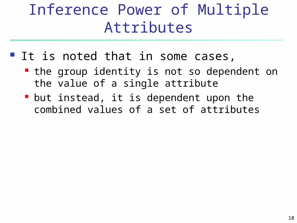
Inference Power of Multiple Attributes

It is noted that in some cases, the group identity is not so dependent on the

value of a single attribute but instead, it is dependent upon the combined

values of a set of attributes

11

Inference Power of Multiple Attributes

In the following table , “a male of low income and a female with high income” drive car neither gender nor income has good inference

powerLabe

lGende

rIncom

eVehicl

e

1 M low car

2 M low car

3 F high car

4 F high car

5 M high bike

6 M high bike

7 F low bike

8 F low bike

12

Algorithm for Inference Power Mining

Feature extraction phase: To learn useful features, which have good

inference powers to group identities, from a subset of the training database.

Feature combination phase: To evaluate extracted features based on the

entire training database and form multi-attribute predicates with good inference powers.

13

Remarks

Note that for the example profile “state” is the attribute with the largest inference

power “beverage” is the attribute with the highest

information gain Information gain considers the cost of the whole

process; hit ratio corresponds to a one-step optimization

14

Extracting Classification Rules from Trees

Represent the knowledge in the form of IF-THEN rules

One rule is created for each path from the root to a leaf

Each attribute-value pair along a path forms a conjunction

The leaf node holds the class prediction Rules are easier for humans to understand

15

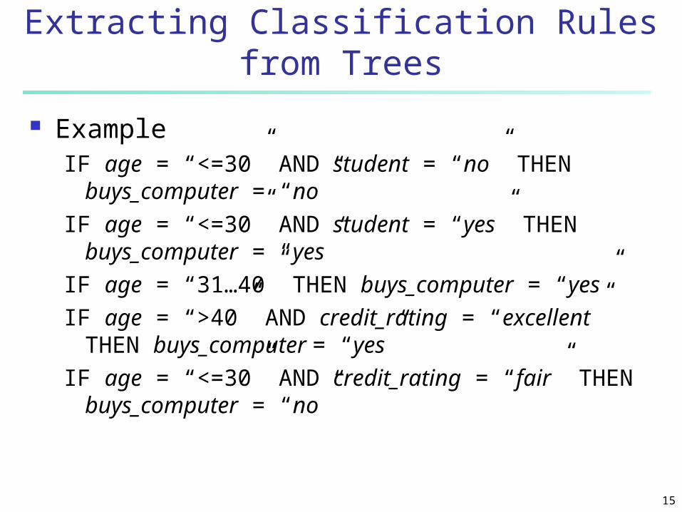
Extracting Classification Rules from Trees

ExampleIF age = “<=30” AND student = “no” THEN

buys_computer = “no”IF age = “<=30” AND student = “yes” THEN

buys_computer = “yes”IF age = “31…40” THEN buys_computer = “yes”IF age = “>40” AND credit_rating = “excellent”

THEN buys_computer = “yes”IF age = “<=30” AND credit_rating = “fair” THEN

buys_computer = “no”

16

Classification in Large Databases

Scalability: Classifying data sets with millions of examples and hundreds of attributes with reasonable speed

Why decision tree induction in data mining? relatively faster learning speed (than other

classification methods) convertible to simple and easy to understand

classification rules comparable classification accuracy with other

methods

17

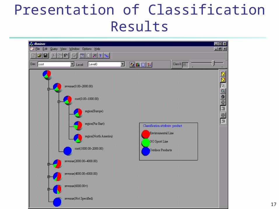
Presentation of Classification Results

18

Visualization of a Decision Tree

19

Neural Networks

Analogy to Biological Systems

Massive Parallelism allowing for

computational efficiency

The first learning algorithm came in 1959

(Rosenblatt) who suggested that if a target

output value is provided for a single neuron

with fixed inputs, one can incrementally

change weights to learn to produce these

outputs

20

A Neuron

The n-dimensional input vector x is mapped into variable y by means of the scalar product and a nonlinear function mapping

k-

f

weighted sum

Inputvector x

output y

Activationfunction

weightvector w

w0w1

wn

x0x1

xn

)sign(y

ExampleFor n

0ikiixw

21

Multi-Layer Feed-Forward Neural Network

Output nodes

Input nodes

Hidden nodes

Output vector

Input vector: xi

22

Given a unit j in a hidden or output layer, the net input, Ij, to unit j is

Given the net input Ij to unit j, then Oj, the output of unit j, is computed as

For a unit j in the output layer, the error Errj is computed by

The error of a hidden layer unit j is

i

jiijj OwI

jIje

O

1

1

))(1( jjjjj OTOOErr

jkk

kjjj wErrOOErr )1(

Multi-Layer Feed-Forward Neural Network

23

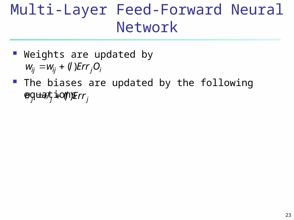
Weights are updated by

The biases are updated by the following equations

jjj Errl)(

Multi-Layer Feed-Forward Neural Network

ijijij OErrlww )(

24

Network Training

The ultimate objective of training obtain a set of weights that makes almost all the

tuples in the training data classified correctly Steps

Initialize weights with random values Feed the input tuples into the network one by one For each unit

Compute the net input to the unit as a linear combination of all the inputs to the unit

Compute the output value using the activation function Compute the error Update the weights and the bias

25

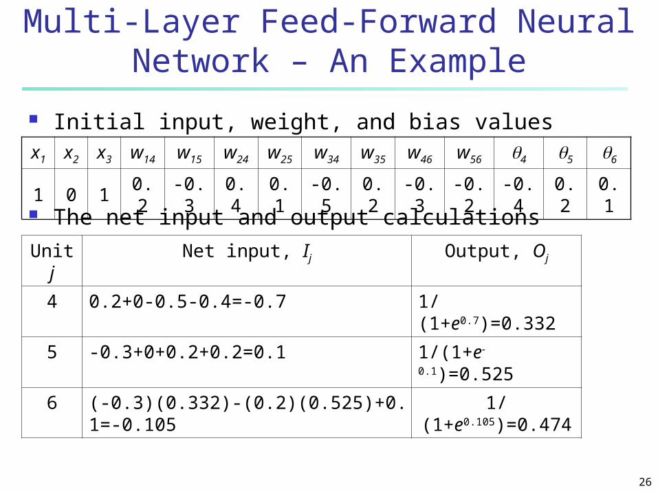
Multi-Layer Feed-Forward Neural Network – An Example

26

Initial input, weight, and bias values

The net input and output calculations

Multi-Layer Feed-Forward Neural Network – An Example

x1 x2 x3 w14 w15 w24 w25 w34 w35 w46 w56 4 5 61 0 1 0.2 -0.3 0.4 0.1 -0.5 0.2 -0.3 -0.2 -0.4 0.2 0.1

Unit j

Net input, Ij Output, Oj

4 0.2+0-0.5-0.4=-0.7 1/(1+e0.7)=0.332

5 -0.3+0+0.2+0.2=0.1 1/(1+e-0.1)=0.525

6 (-0.3)(0.332)-(0.2)(0.525)+0.1=-0.105 1/(1+e0.105)=0.474

27

Calculation of the error at each node

Multi-Layer Feed-Forward Neural Network – An Example

Unit j

Errj

6 (0.474)(1-0.474)(1-0.474)=0.13115 (0.525)(1-0.525)(0.1311)(-0.2)=-0.00654 (0.332)(1-0.332)(0.1311)(-0.3)=-0.0087

28

Calculations for weight and bias updating

Multi-Layer Feed-Forward Neural Network – An Example

Weight or bias

New value

W46 -0.3+(0.9)(0.1311)(0.332)=-0.261W56 -0.2+(0.9)(0.1311)(0.525)=-0.138W14 0.2+(0.9)(-0.0087)(1)=0.192W15 -0.3+(0.9)(-0.0065)(1)=-0.306W24 0.4+(0.9)(-0.0087)(0)=0.4W25 0.1+(0.9)(-0.0065)(0)=0.1W34 -0.5+(0.9)(-0.0087)(1)=-0.508W35 0.2+(0.9)(-0.0065)(1)=0.1946 0.1+(0.9)(0.1311)=0.2185 0.2+(0.9)(-0.0065)=0.1944 -0.4+(0.9)(-0.0087)=-0.408

29

What Is Prediction?

Prediction is similar to classification First, construct a model Second, use model to predict unknown value

Major method for prediction is regression Linear and multiple regression Non-linear regression

Prediction is different from classification Classification refers to predict categorical class

label Prediction models continuous-valued functions

30

Predictive modeling: Predict data values or construct generalized linear models based on the database data.

Method outline: Attribute relevance analysis Generalized linear model construction Prediction

Determine the major factors which influence the prediction Data relevance analysis: uncertainty

measurement, entropy analysis, expert judgment, etc.

Predictive Modeling in Databases

31

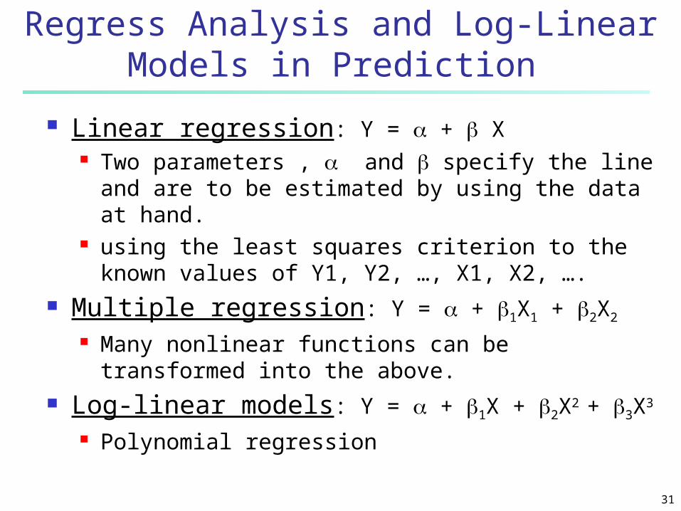
Linear regression: Y = + X Two parameters , and specify the line and

are to be estimated by using the data at hand. using the least squares criterion to the known

values of Y1, Y2, …, X1, X2, …. Multiple regression: Y = + 1X1 + 2X2

Many nonlinear functions can be transformed into the above.

Log-linear models: Y = + 1X + 2X2 + 3X3

Polynomial regression

Regress Analysis and Log-Linear Models in Prediction

32

Summary

Classification is an extensively studied problem

(mainly in statistics, machine learning & neural

networks)

Classification is probably one of the most widely

used data mining techniques with a lot of extensions

Scalability is still an important issue for database

applications: thus combining classification with

database techniques should be a promising topic

Research directions: classification of non-relational

data, e.g., text, spatial, multimedia, etc..