Embed Size (px)
Citation preview

1
Foundations of Software DesignFall 2002Marti Hearst
Lecture 19: B-Trees: Data Structures for Disk

2
Data Structures & Memory
• So far we’ve seen data structures stored in main memory
• What happens when you have a very large set of data?– Too slow to load it into memory– Might not fit into memory
• If you use virtual memory, the paging behavior changes the running time expectations
• A very large array of length N that is stored in virtual memory will take much longer to access if most of data is on pages that are paged out.

3
Data Structures on Disk
• For very large sets of information, we often need to keep most of it on disk
• Examples:– Information retrieval systems– Database systems
• To handle this efficiently:– Keep an index in memory– Keep the data on disk– The index contains pointers to the data on the disk
• Two most common techniques:– Hash tables and B-trees

4
Disk vs. RAM
• Disk has much larger capacity than RAM• Disk is much slower to access than RAM

5Images copyright 2003 Pearson Education
RAM: Memory cells arranged by address

6Images copyright 2003 Pearson Education
Disk: Memory cells arranged by address

7
Disk Structure and Operation
• Made up of platters– Like a phonograph record
• Divided into – tracks (rings) and– sectors (wedges)
• Sectors divided into fixed-sized blocks• As the disk spins beneath it, the read/write arm reads
the data from the block(s) of interest– Data is read into a memory buffer in the OS– This gets eventually transferred to RAM – The process has to wait to get this resource

8
Disk AccessTime
• Seek Time– The time required to move the read/write heads over the disk
surface to the required track.
– Roughly proportional to the distance the heads must move.
• Rotational Latency– The time taken, after the completion of the seek, for the disk platter
to spin until the first sector addressed passes under the read/write heads.
– On average, this is half of a full rotation.
• Transfer Time– The time taken for the disk platter to spin until all the addressed
sectors have passed under the heads.
– Directly proportional to the number of sectors addressed.
Image and text from http://www.ixora.com.au/notes/io_service_times.htm

9
Hash Tables vs. B-Trees
• Hash tables great for selecting individual items– Fast search and insert– O(1) if the table size and hash function are well-chosen
• BUT– Hash tables inefficient for finding sets of information with
similar keys or for doing range searches• (e.g., All documents published in a date range)
– We often need this in text and DBMS applications
• Search trees are better for this– Can place subtrees near each other on disk
• B-Trees are a popular kind of disk-based search tree

10
B-Trees
• Goal: efficient access to sorted information• Balanced Structure• Sorted Keys• Each node has many children• Each node contains many data items
– These are stored in an array in sorted order
• B-Tree is defined in terms of rules:– Makes use of a notion of a constant MINIMUM – These rules can vary
• We’ll use the ones in the Main book

11
B-Tree Rules (from Main)
• Rule 1:– The root may have as few as 1 data item– Every other node has at least MINIMUM items
• Rule 2:– The maximum number of elements in a node is twice
the value of MINIMUM
• Rule 3:– The elements of each B-tree node are stored in a
partially filled array– Sorted from smallest (item 0) to largest

12
B-Tree Rules (from Main)
• Rule 4:– The number of subtrees (children) of a non-leaf node
is always one more than the number of items stored in the node.
• Rule 5:– For any non-leaf node:
(a) A key at index i is greater than all the keys in subtree number i for a given node.
(b) A key at index i is less than all the keys in subtree number i+1 for a given node.
• Rule 6:– Every leaf in a B-tree has the same depth

13
Illustration of Rules 4 and 5
93 and 10793 and 107
Subtree 0Subtree 0 Subtree 1Subtree 1 Subtree 2Subtree 2
all keys < 93 93 <= keys <= 107 107 < all keys
Note: we could use some other ordering here besides integers

14
Example B-tree
66
MINIMUM = 1Does this meet all the rule conditions?
2 and 42 and 4
11 33 55
99
10107 and 87 and 8

15
Implementing B-Trees
• Requires recursive thinking– Every child of the root node is also the root of a
smaller B-tree

16
Example B-tree
66
Each subtree recursively acts like a B-tree.
2 and 32 and 3
44
55
1212
2020 2525
19 and 2219 and 22
6 and 176 and 17
1010 1616 1818
17
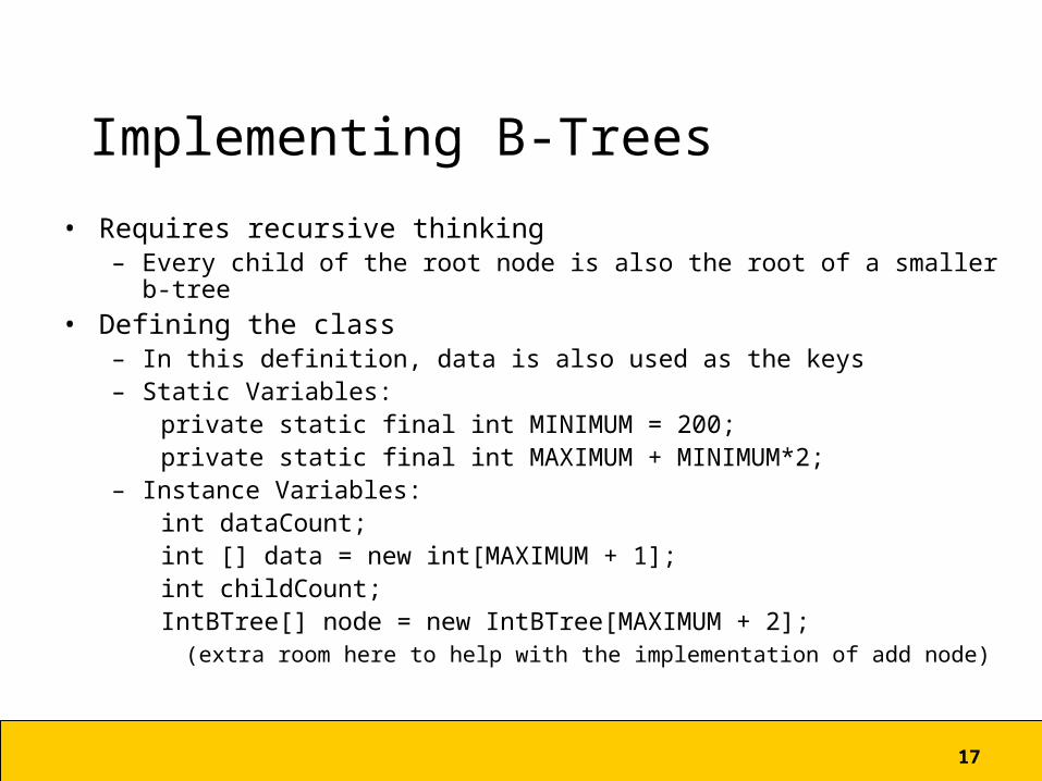
Implementing B-Trees
• Requires recursive thinking– Every child of the root node is also the root of a smaller b-tree
• Defining the class– In this definition, data is also used as the keys– Static Variables:
private static final int MINIMUM = 200;private static final int MAXIMUM + MINIMUM*2;
– Instance Variables:int dataCount;int [] data = new int[MAXIMUM + 1];int childCount;IntBTree[] node = new IntBTree[MAXIMUM + 2];
(extra room here to help with the implementation of add node)

18
Searching for an Item
boolean contains (int target, IntBTree node)set i equal to the first index in node such that
data[i] >= target
if (target found at data[i]) return true
else if (node has no children)return false
else return node[i].contains(target)

19
Find 18?
66
2 and 32 and 3
44
55
1212
2020 2525
19 and 2219 and 22
6 and 176 and 17
1010 1616 1818
boolean contains (int target, IntBTree node)
set i equal to the first index in node such that
data[i] >= target
if (target found at data[i])
return true
else if (node has no children)
return false
else
return node[i].contains(target)

20
Adding a Node
• Tricky because of the need to maintain the B-Tree rules
• The strategy:– First place the new item wherever it belongs,
according to the value of the key– Then if a node has too many items, recursively
split the too-large node until the B-Tree condition is recovered.
21
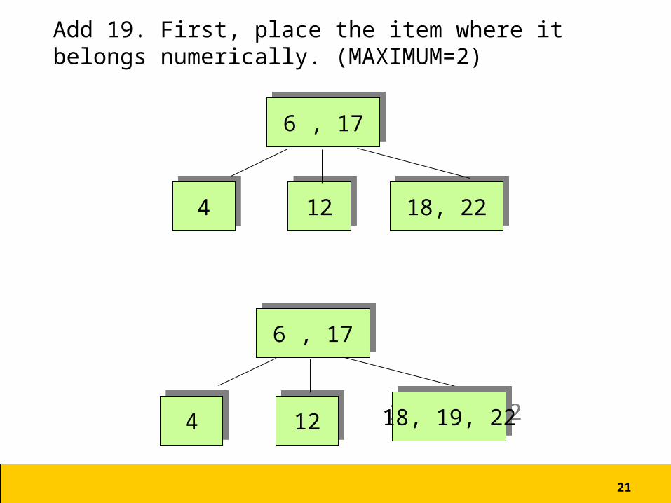
Add 19. First, place the item where it belongs numerically. (MAXIMUM=2)
44 1212 18, 2218, 22
6 , 176 , 17
44 1212
6 , 176 , 17
18, 19, 2218, 19, 22

22
Now Propagate extra item up a level to restore the B-Tree condition.
66
44 1212 18, 19, 2218, 19, 22
6 , 176 , 17
44 1212
6 , 17, 196 , 17, 19
1818 2222
Requires a node split
23
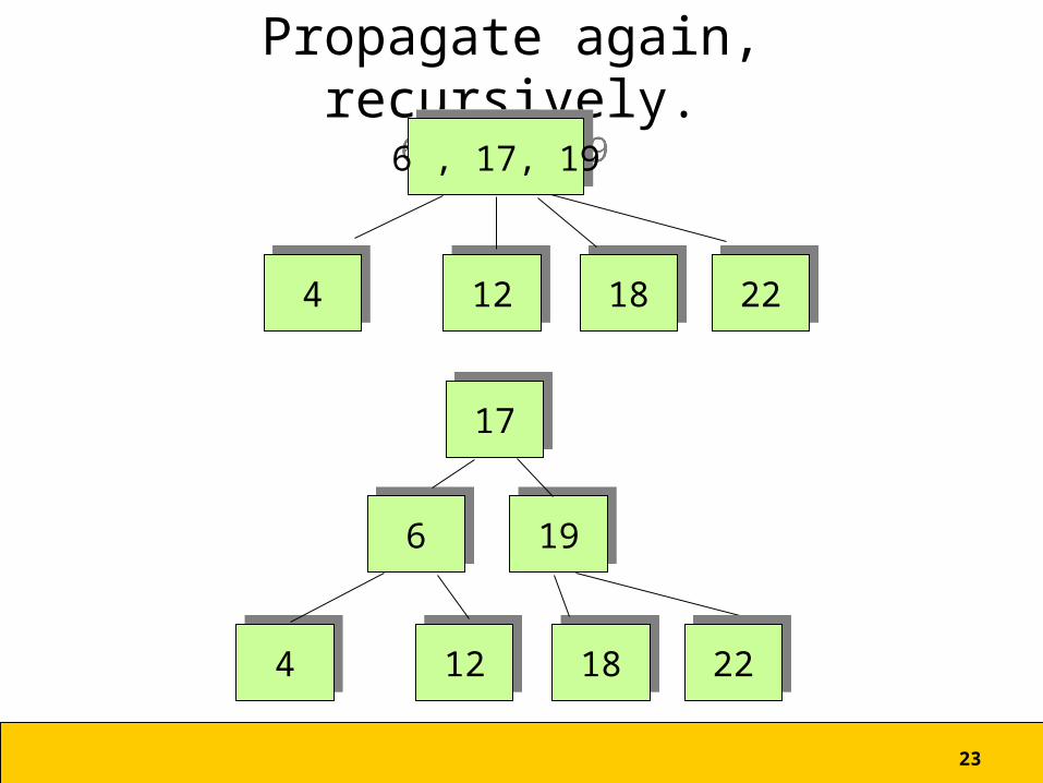
Propagate again, recursively.
66
44 1212
6 , 17, 196 , 17, 19
1818 2222
66
44 1212 1818 2222
1919
1717

24
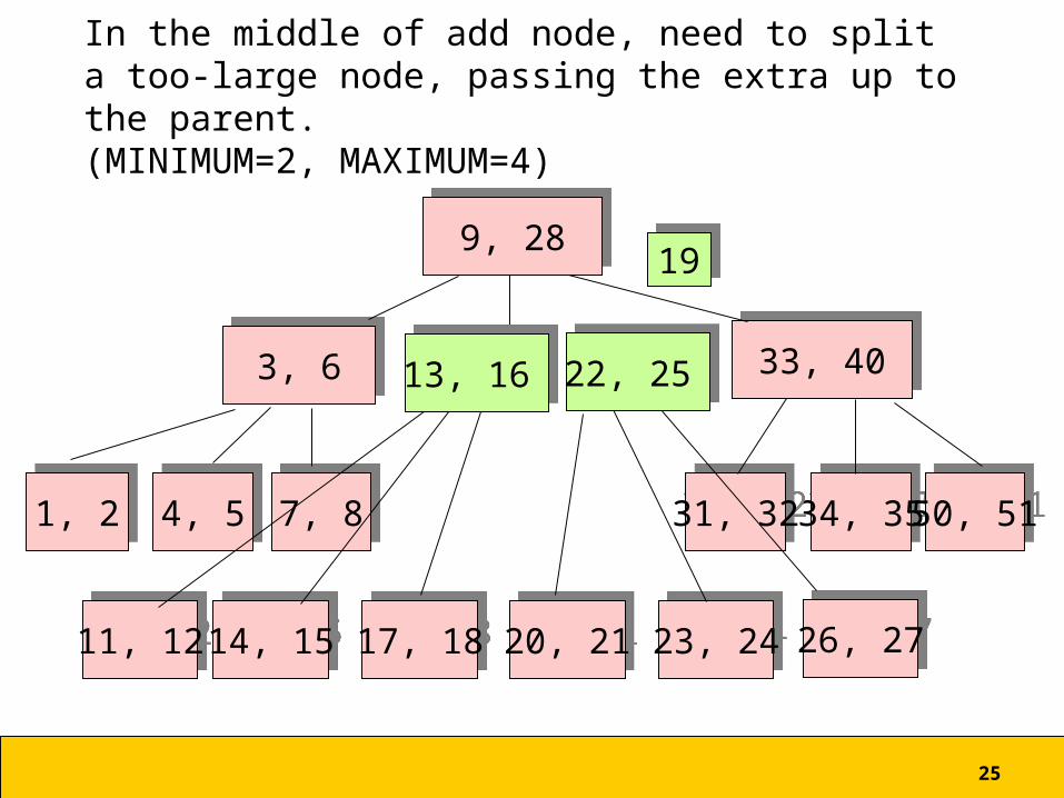
In the middle of add node, need to split a too-large node, passing the extra up to the parent.(MINIMUM=2, MAXIMUM=4)
66
1, 21, 2
3, 63, 6
7, 87, 8
13, 16, 19, 22, 2513, 16, 19, 22, 25
34, 3534, 35 50, 5150, 51
33, 4033, 40
9, 289, 28
14, 1514, 15
31, 3231, 324, 54, 5
17, 1817, 18 20, 2120, 21 23, 2423, 24 26, 2726, 2711, 1211, 12
25
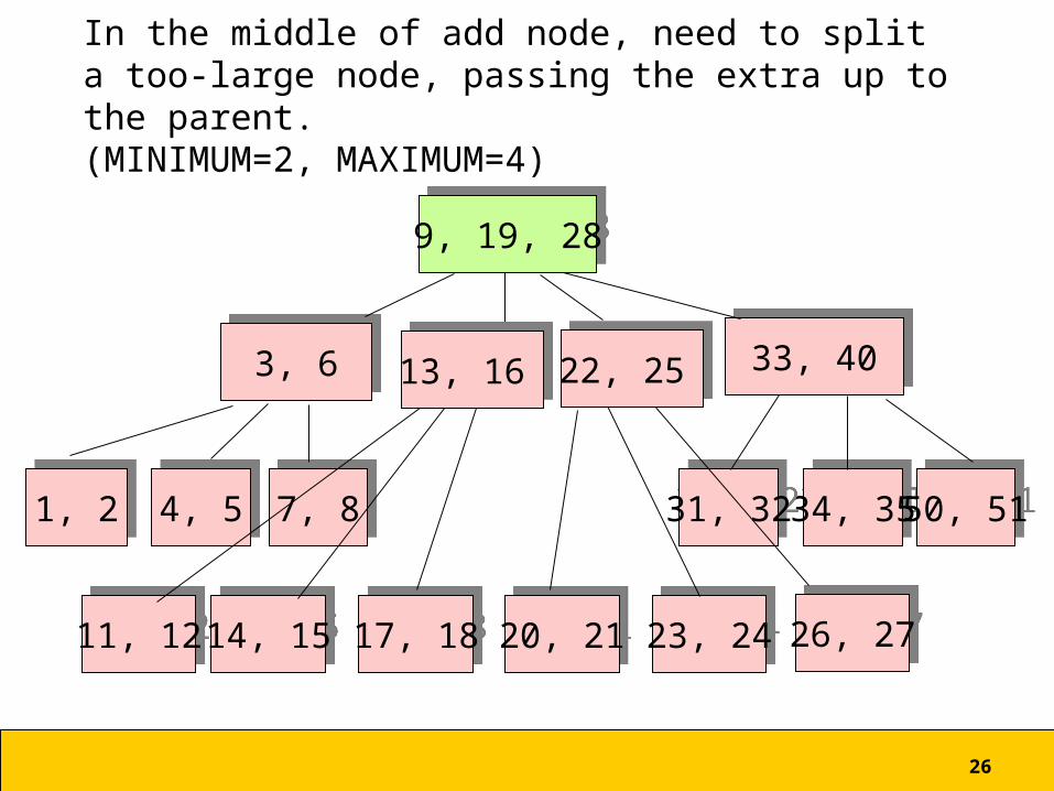
In the middle of add node, need to split a too-large node, passing the extra up to the parent.(MINIMUM=2, MAXIMUM=4)
66
1, 21, 2
3, 63, 6
7, 87, 8 34, 3534, 35 50, 5150, 51
33, 4033, 40
9, 289, 28
14, 1514, 15
31, 3231, 324, 54, 5
17, 1817, 18 20, 2120, 21 23, 2423, 24 26, 2726, 2711, 1211, 12
13, 16 13, 16 22, 25 22, 25
1919
26
In the middle of add node, need to split a too-large node, passing the extra up to the parent.(MINIMUM=2, MAXIMUM=4)
66
1, 21, 2
3, 63, 6
7, 87, 8 34, 3534, 35 50, 5150, 51
33, 4033, 40
9, 19, 289, 19, 28
14, 1514, 15
31, 3231, 324, 54, 5
17, 1817, 18 20, 2120, 21 23, 2423, 24 26, 2726, 2711, 1211, 12
13, 16 13, 16 22, 25 22, 25
27
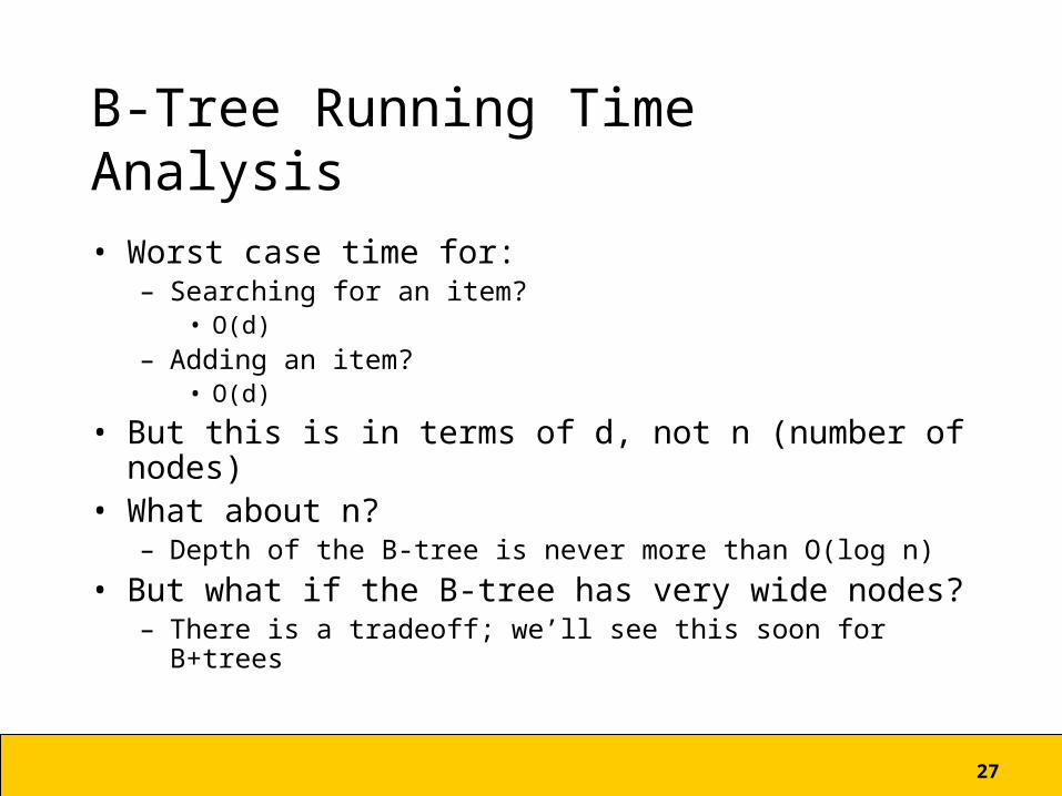
B-Tree Running Time Analysis
• Worst case time for:– Searching for an item?
• O(d)– Adding an item?
• O(d)
• But this is in terms of d, not n (number of nodes)
• What about n?– Depth of the B-tree is never more than O(log n)
• But what if the B-tree has very wide nodes?– There is a tradeoff; we’ll see this soon for B+trees

28Slide adapted from cis.stvincent.edu
B+Trees
• Differences from B-Tree – Assume the actual data is in a separate file on disk– Internal nodes store keys only
• Each node may contain many keys• Designed to be “branchy” or “bushy”• Designed to have shallow height• Has a limit on the number of keys per node
– This way only a small number of disk blocks need to be read to find the data of interest
– Only leaves store data records• The leaf nodes refer to memory locations on disk• Each leaf is linked to an adjacent leaf

29
B+Tree and Disk Reads
• Goal:– Optimize the B+tree structure so that a minimum
number of disk blocks need to be read
• If the number of keys is not too large, keep all of the B+tree in memory
• Otherwise, – Keep the root and first levels of nodes in memory– Organize the tree so that each node fits within a disk
block in order to reduce the number of disk reads

30Slide adapted from lecture by Hector Garcia-Molina
B+tree rules tree of order s
(1) All leaves at same lowest level(balanced tree)
(2) Pointers in leaves point to recordsexcept for “sequence pointer”

31Slide adapted from lecture by Hector Garcia-Molina
B+Tree Sizes
• Size of nodes:s keyss+1 pointers
• Don’t want nodes to be too emptyUse at least:
Non-leaf: (s+1)/2 pointersLeaf: (s+1)/2 pointers to data

32Slide adapted from lecture by Hector Garcia-Molina
Root
B+Tree Example s=3
100
120
150
180
30
3 5 11
30
35
100
101
110
120
130
150
156
179
180
200
33Slide adapted from lecture by Hector Garcia-Molina
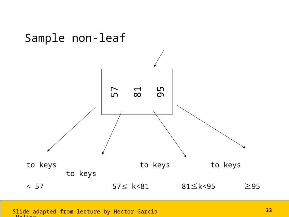
Sample non-leaf
to keys to keys to keys to keys
< 57 57 k<81 81k<95 95
57
81
95
34Slide adapted from lecture by Hector Garcia-Molina
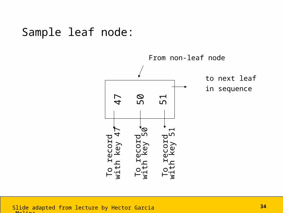
Sample leaf node:
From non-leaf node
to next leafin sequence
47
50
51
To r
eco
rd
wit
h k
ey 4
7
To r
eco
rd
wit
h k
ey 5
0
To r
eco
rd
wit
h k
ey 5
1

35Slide adapted from lecture by Hector Garcia-Molina
Full node min. node
Non-leaf
Leaf
s=3
12
01
50
18
0
30
3 5 11
30
35
36
Example Use of B+Trees• Recall that an inverted index is composed of
– A Dictionary file and – A Postings file
• Use a B+Tree for the dictionary– The keys are the words– The values stored on disk are the postings

37
Using B+Trees for Inverted Index
• Use it to store the dictionary• More efficient for searches on words with the
same prefix– count* matches count, counter, counts, countess
– Can store the postings for these terms near one another
– Then only one disk seek is needed to get to these

38
Inverted Index
Dictionary PostingsDoc # Freq
2 11 11 12 11 11 12 12 11 11 12 11 12 12 11 12 12 11 11 12 12 11 22 21 11 12 11 22 2
Term N docs Tot Freqa 1 1aid 1 1all 1 1and 1 1come 1 1country 2 2dark 1 1for 1 1good 1 1in 1 1is 1 1it 1 1manor 1 1men 1 1midnight 1 1night 1 1now 1 1of 1 1past 1 1stormy 1 1the 2 4their 1 1time 2 2to 1 2was 1 2
39Slide adapted from lecture by Hector Garcia-Molina
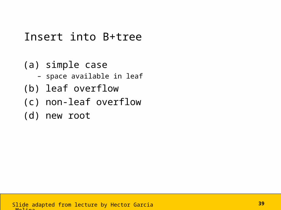
Insert into B+tree
(a) simple case– space available in leaf
(b) leaf overflow(c) non-leaf overflow(d) new root

40Slide adapted from lecture by Hector Garcia-Molina
(a) Insert key = 32 s=33 5 11
30
31
30
100
32

41Slide adapted from lecture by Hector Garcia-Molina
(a) Insert key = 7 s=3
3 5 11
30
31
30
100
3 5
7
7

42Slide adapted from lecture by Hector Garcia-Molina
(c) Insert key = 160 s=3
10
0
120
150
180
150
156
179
180
200
160
18
0
160
179

43Slide adapted from lecture by Hector Garcia-Molina
(d) New root, insert 45 s=3
10
20
30
1 2 3 10
12
20
25
30
32
40
40
45
40
30new root

44Slide adapted from lecture by Hector Garcia-Molina
Interesting problem:
For B+tree, how large should s be?
…
n is number of keys / node

45
What is the expected running time for finding an item in the B+tree?
• Assume B+tree with nodes of size s• Assume all of the index is in memory
– Use binary search to locate the appropriate key within a node• This takes a + b log2 s for constants a and b• Remember that s is a constant
• Assume the B+tree is full– # nodes to examine is logs n where n = # records
• If n dominates– (Meaning that the tree is deeper than the nodes are wide)– O(logs n)
• If s dominates– (Meaning the nodes are wider than the tree is deep)– O(log2s)

46Slide adapted from lecture by Hector Garcia-Molina
Sample assumptions: (order s B+tree)
(1) Time to read node from disk is(70+0.05s) msec.
(2) Once block in memory, use binarysearch to locate key:
(a + b log2 s) msec.
For some constants a,b; Assume a << 70
(3) Assume B+tree is full, i.e., # nodes to examine is logs nwhere n = # records

47Slide adapted from lecture by Hector Garcia-Molina
Can get: f(s) = time to find a record
f(s)
sopt s
Thus if s is too big or too small, problems result

48Slide adapted from lecture by Hector Garcia-Molina
FIND sopt by f’(s) = 0
Answer is sopt = “few hundred”
What happens to sopt as
• Disk gets faster?• CPU gets faster?
49Slide adapted from lecture by Hector Garcia-Molina
Tradeoffs:
B-trees have faster lookup than B+trees
But B+Tree is faster lookup if using fixed-sized blocks
In B-tree, deletion more complicated
B+trees often preferred

50
Choosing Data Structures
• Name example applications best suited for– Hash Tables– B+Trees
51
Next Time
• Sorting Algorithms