1

Citation: Cheng, N. S. (2008). “Formulas for friction factor in transitional regions.” Journal of Hydraulic Engineering, ASCE, 134(9), 1357-1362.

Formulas for friction factor in transitional regimes

Nian-Sheng Cheng

School of Civil and Environmental Engineering, Nanyang Technological University

Nanyang Avenue, Singapore 639798. Email: cnscheng@ntu.edu.sg

Abstract: This note concerns variations of the friction factor in the two transitional

regimes, one between laminar and turbulent flows and the other between fully-smooth

and fully-rough turbulent flows. An interpolation approach is developed to derive a single

explicit formula for computing the friction factor in all flow regimes. The results obtained

for pipe flows give a better representation of Nikuradse’s experimental data, in

comparison with other implicit formulas available in the literature. Certain modifications

are also made for applying the obtained friction formula to open channel flows.

Keywords: friction factor, transition, pipe flow, open channel flow, interpolation,

laminar flow, turbulent flow, Reynolds number, resistance

2

Introduction

Nikuradse (1933) conducted his notable series of flow measurements with smooth and

rough pipes over a wide range of Reynolds numbers. As a benchmark in hydraulic

engineering, these measurements have served as a crucial database for verifying

formulations developed for velocity profiles and flow resistance. In particular,

Nikuradse’s work also offers valuable information for investigating sediment transport

phenomena because similar sand-roughened boundaries are often employed for the

laboratory study of various open channel flows over sediment beds.

The friction factor derived from Nikuradse’s experimental data appears to be

different from the widely-used Moody diagram in that Nikuradse’s data show a ‘dip’ in

the friction factor for turbulent pipe flows in the intermediate Reynolds number between

fully-rough and fully-rough regimes. The dip phenomenon has been attributed to the pipe

wall roughened by well-sorted sand particles, and it may become insignificant in

commercial pipes with non-uniform distribution of roughness elements (Colebrook 1939).

Similar transitional effects were also observed for other regular roughness configurations

(Jimenez 2004). However, many fluid mechanics textbooks choose to start with

Nikuradse’s experimental results for discussing different flow conditions and then

recommend the Moody diagram for practical uses, but with almost no efforts devoted to

explain and quantify the dip phenomenon (Bradshaw 2000).

Several formulas have been proposed in the literature for computing the friction

factor separately for laminar flows, and fully-smooth and fully-rough turbulent flows, but

they are not applicable directly for the transitional regimes (Hinze 1975). Some others,

3

although applicable for the transitional regimes, need a trial procedure for estimating the

friction factor (e.g. Brownlie 1981; Cheng and Chiew 1998; Ligrani and Moffat 1986;

Yalin and Da Silva 2001). However, for practical purposes such as computer applications,

a single friction equation that applies for all flow regimes is often required. Yen (2002)

considered that this could be established with certain probability-based considerations. In

this note, an interpolation method, which could be considered probability-related, is

developed to derive a single explicit formula for computing the friction factor for various

flow conditions including the transitional regimes.

Interpolation method

First, we consider the transition between laminar and turbulent flows, in which the

variation of the friction factor is composed of laminar and turbulent components. It is

assumed that the friction factor, f, is given by

α−α= 1TL fff (1)

where fL is the friction factor for laminar flows, fT is that for turbulent flows, and α is the

weighting factor. The friction factor here is given by 8(u*/V)0.5, where u* is the friction

velocity and V is the cross-sectional mean velocity. In the sense of Yen’s (2002)

probability conjecture, α can be considered the probability of the effect of the laminar

component on the friction, and (1-α) the probability of the contribution of the turbulent

component. Extremely, the flow remains in the laminar regime at α = 1 and switches to

the turbulent regime at α = 0. As a result, α is somehow related to the mechanism of

4

intermittency and thus depends on the Reynolds number, Re (= VD/ν) where D is the pipe

diameter and ν is the kinematic viscosity of fluid.

For turbulent flows, the friction factor varies with the Reynolds number and also

can be altered by boundary roughness. At intermediate Reynolds numbers, a transitional

regime exists between fully-smooth and fully-rough turbulent flows. To follow the

approach in dealing with the laminar to turbulent flow transition, it is further assumed

that

β−β= 1TRTST fff (2)

where fTS is the friction factor for fully-smooth turbulent flows, fTR is that for fully-rough

turbulent flows and β is the weighting factor. In terms of probability, β is used here to

quantify the possible effect of the fully-smooth component on the turbulent friction while

(1-β) is used to describe the possible effect of the fully-rough component. Therefore, β

depends generally on the Reynolds number and boundary roughness height.

Substituting Eq. (2) into Eq. (1), we arrive at

)1)(1()1( β−α−βα−α= TRTSL ffff (3)

To individually compute the three friction factors, fL, fTS and fTR, we may use the

following established results (Hinze 1975),

Re

fL64

= for laminar pipe flows, (4)

2

5122

−

⎟⎟⎠

⎞⎜⎜⎝

⎛=

.Ref

logf TSTS for fully-smooth turbulent pipe flows, and (5)

5

2

7.3log2−

⎟⎟⎠

⎞⎜⎜⎝

⎛=

sTR k

Df for fully-rough turbulent pipe flows. (6)

where ks is the roughness size that is taken as the sand grain diameter for Nikuradse’s

experiments. Eq. (5) is the Prandtl’s friction law for smooth pipes and Eq. (6) is the von

Karman’s formula for the fully rough regime. Since it involves a trial procedure in

computing the friction factor, Eq. (5) is replaced here with

2

8.6log8.1

−

⎟⎠⎞

⎜⎝⎛=

RefTS (7)

Eq. (7), except for the constant 6.8 included, is the same as that previously given by

Colebrook (1939). Other approximations similar to Eq. (7) were also reported by Barr

(1977), Swamee and Jain (1976) and Haaland (1983). However, a best-fit analysis

conducted in this study shows that Eq. (7) differs from Eq. (5) within ±1.2% for Re =

4000-108, performing the best when compared with the other studies.

Substituting Eqs. (4), (6) and (7) into Eq. (3), the friction factor for pipes

roughened by well-sorted sand grains is given by

)1)(1(2)1(2 7.3log2

8.6log8.1

641

β−α−βα−α

⎟⎟⎠

⎞⎜⎜⎝

⎛⎟⎠⎞

⎜⎝⎛

⎟⎠⎞

⎜⎝⎛=

skDReRe

f (8)

Evaluation of α and β

First, we define an intermediate Reynolds number, ReLT, at which the flow transition

occurs between laminar and turbulent regimes. If Re is much smaller than ReLT, the flow

is largely characterised as laminar and thus α → 1 based on Eq. (1). Otherwise, the flow

6

is dominantly turbulent and α → 0 if Re is much greater than ReLT. With this

consideration, the value of α would reduce with an increase in the ratio of Re/ReLT.

Mathematically, the relationship could be described by

mLTReRe )/(1

1+

=α (9)

where m is an exponent. Eq. (9) predicts α in the range of 0 to 1. At Re = ReLT, α = 0.5

and thus TL fff = following Eq. (1), which implies that the contributions by the

laminar and turbulent components are equivalent. This further suggests that ReLT could be

slightly greater than the critical Reynolds number at which the laminar flow just loses its

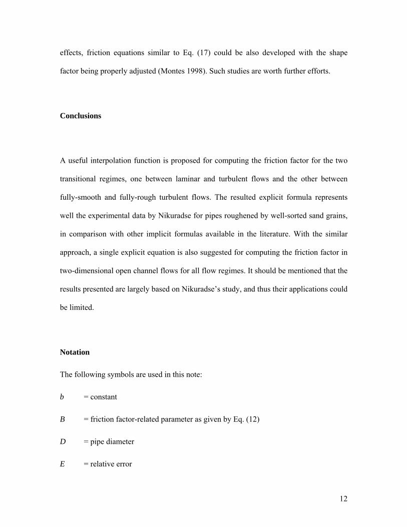
stability. In this study, both ReLT and m are evaluated by fitting Eq. (8) to Nikuradse’s

data, with α given by Eq. (9) and β = 1. This yields that ReLT ≈ 2720 and m ≈ 9. The

comparison is shown in Fig. 1. Also superimposed on the figure are Eq. (4) for laminar

flows and Eq. (5) together with its approximation, Eq.(7), for fully-smooth turbulent

flows.

Similarly, to estimate β, we engage another intermediate Reynolds number,

denoted by ReSR, which is associated with the transition between fully-smooth and fully-

rough turbulent flows. Different from ReLT that appears as a constant, ReSR varies with the

relative roughness, r/ks. From Eq. (2), it follows that β decreases from 1 to 0 if the

turbulent flow changes from the fully-smooth to fully-rough regime. Therefore, it is

reasonable to believe that β would reduce with an increase in the ratio of Re/ReSR,

approximately, in the form

7

nSRReRe )/(1

1+

=β (10)

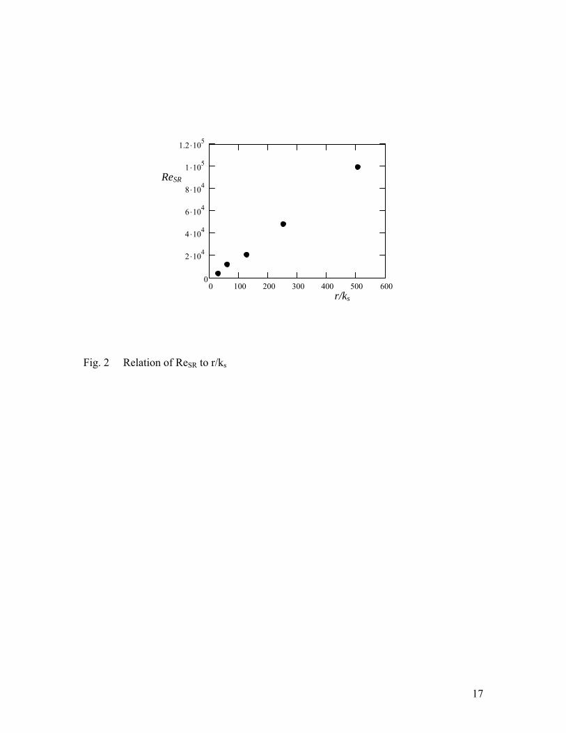
where n is an exponent. Next, it is necessary to know how ReSR varies with r/ks. By

taking ReSR to be a Reynolds number halfway in the transition for a given r/ks and using

Tables 2-7 of Nikuradse (1933), one can get that ReSR increases with increasing r/ks. The

result so estimated is plotted in Fig. 2, which shows that the relation of ReSR to r/ks is

almost linear. Consequently, by assuming that ReSR = ηr/ks with η being a constant, Eq.

(10) can be rewritten as

nskrRe )]//([1

1η+

=β (11)

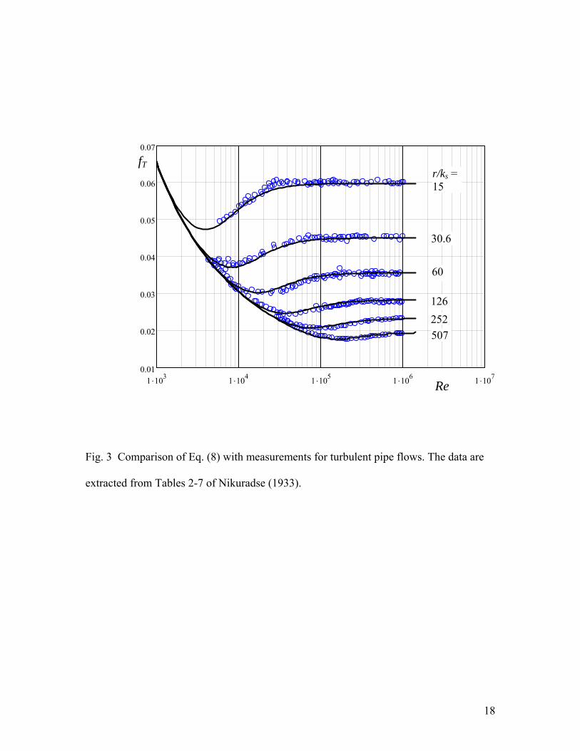
With β given by Eq. (11) and also taking α = 0 for turbulent pipe flows, comparing Eq.

(8) with Nikuradse’s data yields that η ≈ 320 and n ≈ 2, as presented in Fig. 3.

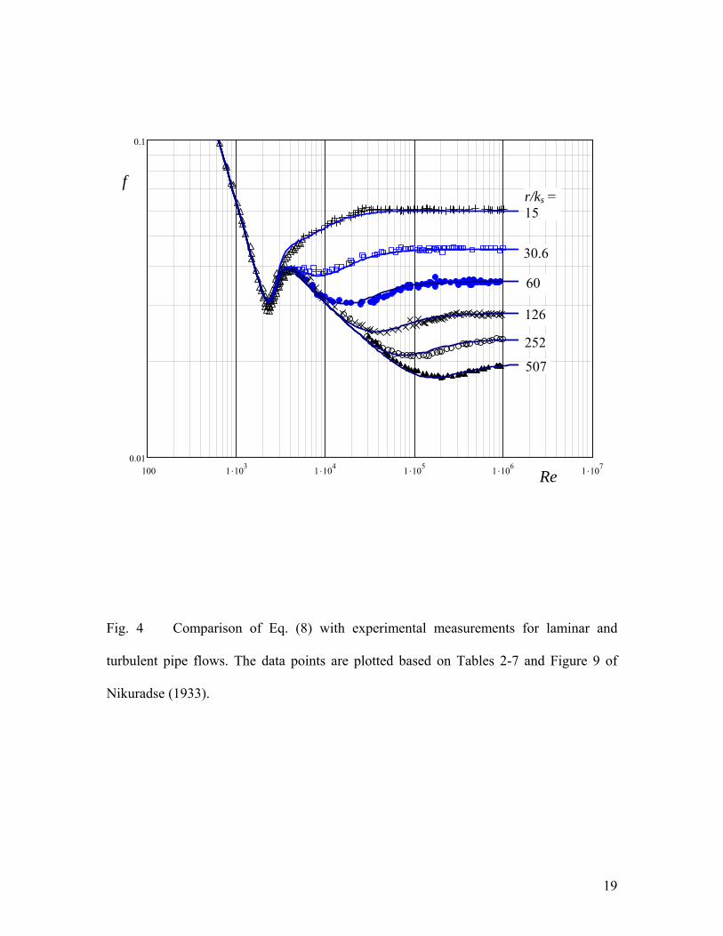
Finally, with α and β given by Eqs. (9) and (11) respectively, Eq. (8) is compared

with the entire database by Nikuradse (1933) for smooth pipes and rough pipes with r/ks

ranging from 15 to 507. As shown in Fig. 4, Eq. (8) represents well the experimental

data.

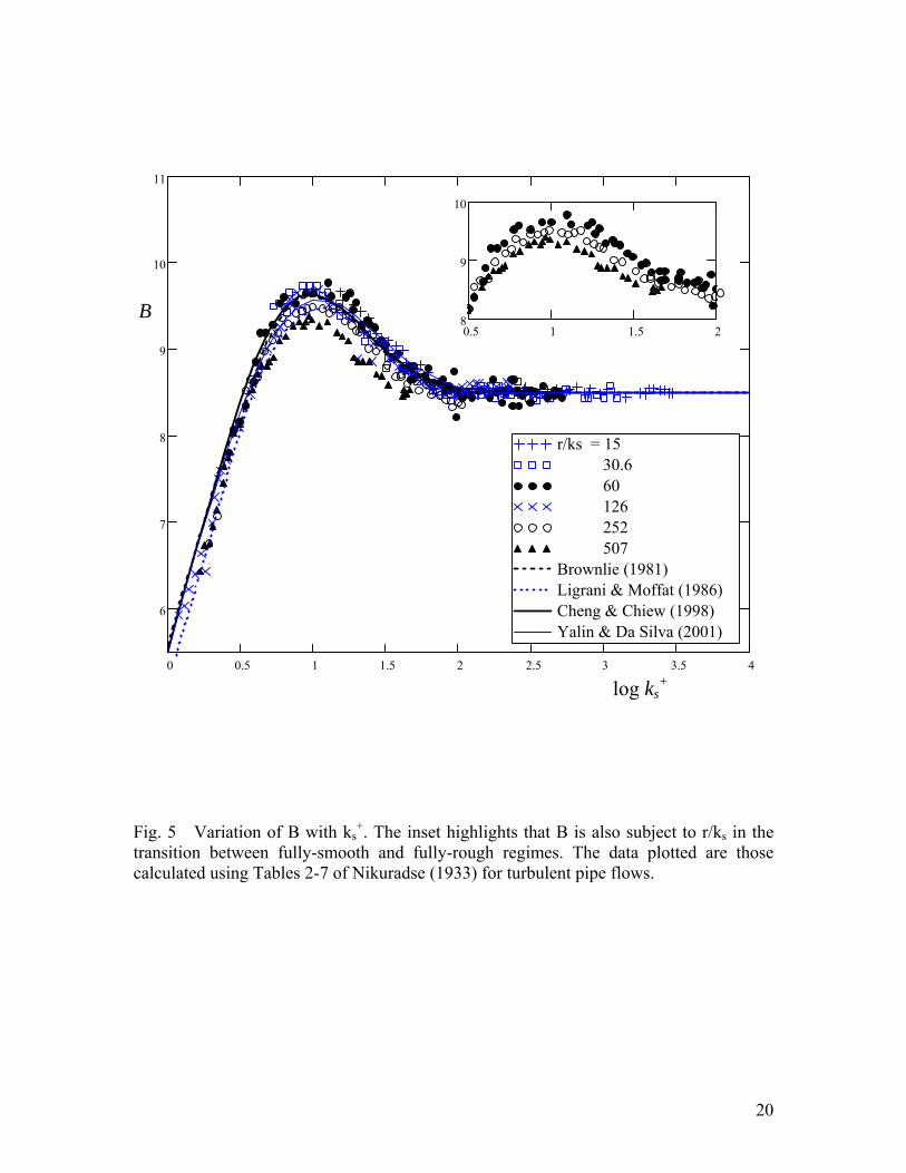
Comparison with previous studies

In the literature, there are no single formulas that are available to explicitly calculate the

friction factor in various flow regimes to the writer’s knowledge. However, several

empirical equations have been proposed for computing the function, B, which is related

8

to f in the following form (e.g. Brownlie 1981; Cheng and Chiew 1998; Ligrani and

Moffat 1986; Yalin and Da Silva 2001),

75.3log21875.3ln5.28+

⎥⎥⎦

⎤

⎢⎢⎣

⎡⎟⎟⎠

⎞⎜⎜⎝

⎛−=+⎟⎟

⎠

⎞⎜⎜⎝

⎛−=

ss kr

fkr

fB (12)

Eq. (12) is derived by integrating the log law, u/u* = 2.5ln(y/ks) + B, over the cross

section of pipe. It should be mentioned that a trial procedure is required when using Eq.

(12) for the evaluation of the friction factor because B is usually presented as a function

of the roughness Reynolds number, ks+, which is defined as ν/* sku and equal to

ReDkf s )/(8/ .

The following four formulas are used to compare with the present study:

(1) Brownlie’s (1981) formula

( )⎪⎪

⎩

⎪⎪

⎨

⎧

>

≤≤

<+

=−

+

+

=

+

++

∑10074.1

10010log

10log2705.0

8

6

0

s

si

isi

ss

kfor

kforka

kforkbB (13)

where the coefficients, ai (i = 0-6), are 1.3376, -4.3218, 19.454, -26.48, 16.590, -4.9407

and 0.57864, respectively, and b is taken as 3.58 by ensuring that B ≈ 8.5 for ks+ > 100.

(2) Ligrani and Moffat’s (1986) formula s

⎪⎪

⎩

⎪⎪

⎨

⎧

>

≤≤⎟⎟⎠

⎞⎜⎜⎝

⎛ π−++

<+

=

+

++

++

++

905.8

9025.2)25.2/90ln(2)25.2/ln(sin)ln5.24.3(ln5.21.5

25.2ln5.21.5

s

ss

ss

ss

kfor

kforkkk

kfork

B (14)

(3) Cheng and Chiew’s(1998) formula

9

( )[ ]5.2ln11.0exp)3ln5.2(5.8 ++ −−+= ss kkB (15)

(4) Yalin and Da Silva’s (2001) formula

( )[ ] ( )[ ]⎭⎬⎫

⎩⎨⎧ −−+−+= +++ 55.255.2 ln0594.0exp15.8ln0705.0exp)5.5ln5.2( sss kkkB (16)

Eqs. (13) to (16) are plotted in Fig. 5 together with Nikuradse’s data. All formulas predict

smooth variations of B with ks+, while the experimental data fluctuate particularly in the

transitional regime, say, for 5 < ks+ < 70. The scattering of the data points, perhaps

partially due to experimental uncertainties, is clearly associated with the variation in r/ks,

as highlighted in the inset of Fig. 5. However, this r/ks-dependence cannot be described

by the previous formulas, which all relate B to ks+ only. In addition, it should be

mentioned here that the data series with r/ks = 507, which clearly deviates from the main

data trend, was not presented in the graph provided originally by Nikuradse (1933) and

cited subsequently by others (e.g. Hinze 1975; Schlichting 1979) .

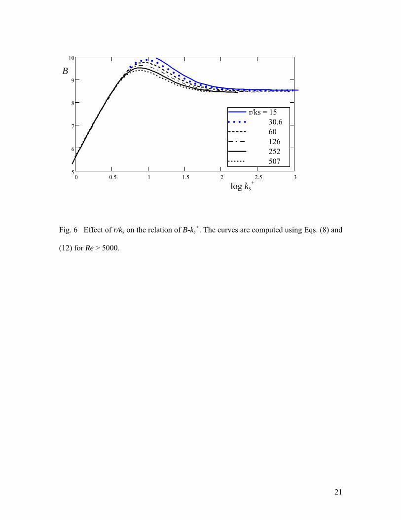
In the following, the friction factor is first computed using Eq. (8) for Re > 5000,

and then substituted into Eq. (12) for evaluating B. The result obtained is plotted in Fig.

6. It shows that the effect of r/ks is not significant for very small and very large ks+, but

becomes considerable in the transitional regime. This observation is consistent with

Nikuradse’s measurements, as shown in Fig. 5.

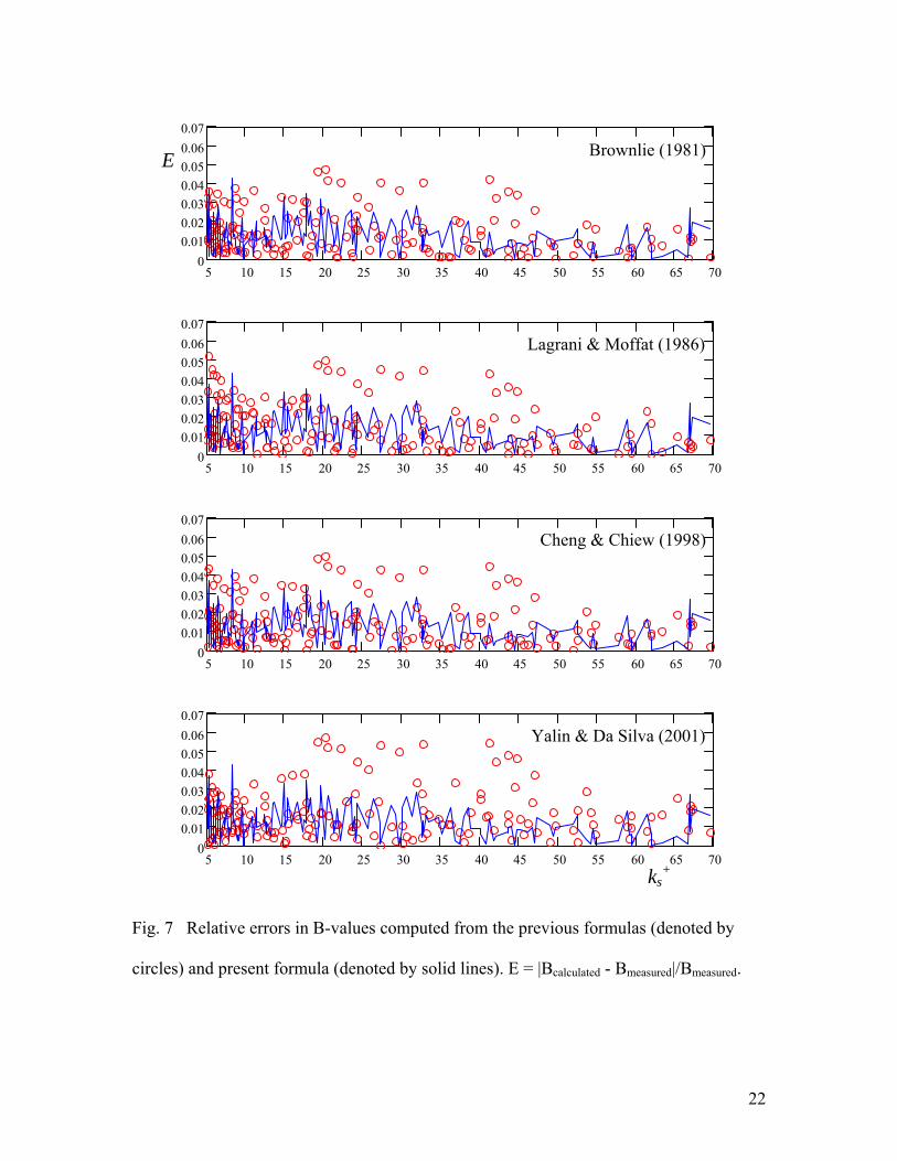
Fig. 7 further details the difference between the B-values calculated with the

current approach and those by the previous formulas for 5 < ks+ < 70. In this figure, the

vertical coordinate is defined as the relative error, E = ⏐Bcalculated – Bmeasured⏐/Bmeasured,

where Bmeasured is obtained through Eq. (12) from the friction factor measurements by

Nikuradse (1933). The results indicate that the prediction errors are generally not more

10

than 6%, but the present approach provides the best accuracy because of taking into

account the effect of r/ks. The average errors associated with Eqs. (13) to (16) are 1.4%,

1.5%, 1.7% and 1.5%, respectively, while that by the present study is 1.2%. The

maximum errors associated with Eqs. (13) to (16) are 4.7%, 5.2%, 5.8% and 5.0%,

respectively, while that by the present study is 4.3%.

Extension to open channel flows

To extend experimental or theoretical results that are obtained for pipe flows to open

channel flows, one may use the concept of equivalent hydraulic radius, which is equal to

D/4 for circular pipe flows and h, the flow depth, for wide open channel flows. However,

practical applications of this concept indicate that further modifications are needed for

computing the friction factor. For example, a shape factor, φ, could be used to effectively

account for the influence of the cross section when applying the pipe resistance equations

to open channels of any shape (Montes 1998). This shape factor is used as a multiplier for

the hydraulic radius. For two-dimensional (2D) open channel flows, φ is equal to

approximately 0.8, and thus the hydraulic radius, i.e. D/4, included in the pipe friction

equations should be replaced with 0.8h. Another similar idea for estimating turbulent

friction in noncircular ducts is to use the pipe-friction law based on an effective diameter

(White 1991).

In this study, the concept of the shape factor is adopted. Therefore, D included in

Eqs. (6) and (7) should be replaced with 4 × (0.8h) = 3.2h for 2D open channel flows.

11

However, this change is only limited to turbulent flows and does not apply for the

laminar friction. For 2D open channel flows, the laminar friction factor is given by fL =

24/Reh, which can be derived from the parabolic velocity distribution. Here, the depth-

averaged velocity U is used for defining the Reynolds number Reh (=Uh/ν), h is the flow

depth, and the friction factor f is redefined as 8(u*/U)2. With these considerations, Eq. (8)

is rewritten as

)1)(1(2)1(2 8.11log2

1.2log8.1

241

β−α−βα−α

⎟⎟⎠

⎞⎜⎜⎝

⎛⎟⎠⎞

⎜⎝⎛

⎟⎠⎞

⎜⎝⎛=

s

hh

khReRe

f (17)

In Eq. (17), the two constants, 2.1 and 11.8, are obtained here based on the concept of the

shape factor, but they are almost the same as those suggested by Yen (2002). This implies

that the approach based on the shape factor, although empirical, provides a reasonable

connection between the friction factor in pipe flows and that in 2D open channel flows.

Therefore, it is reasonable to apply the same approach for the evaluation of the α and β

values, which are proposed for the transitional regimes. This yields that Eqs. (9) and (11),

are rewritten as

9)850/(11

hRe+=α (18)

2)]/160/([11

sh khRe+=β (19)

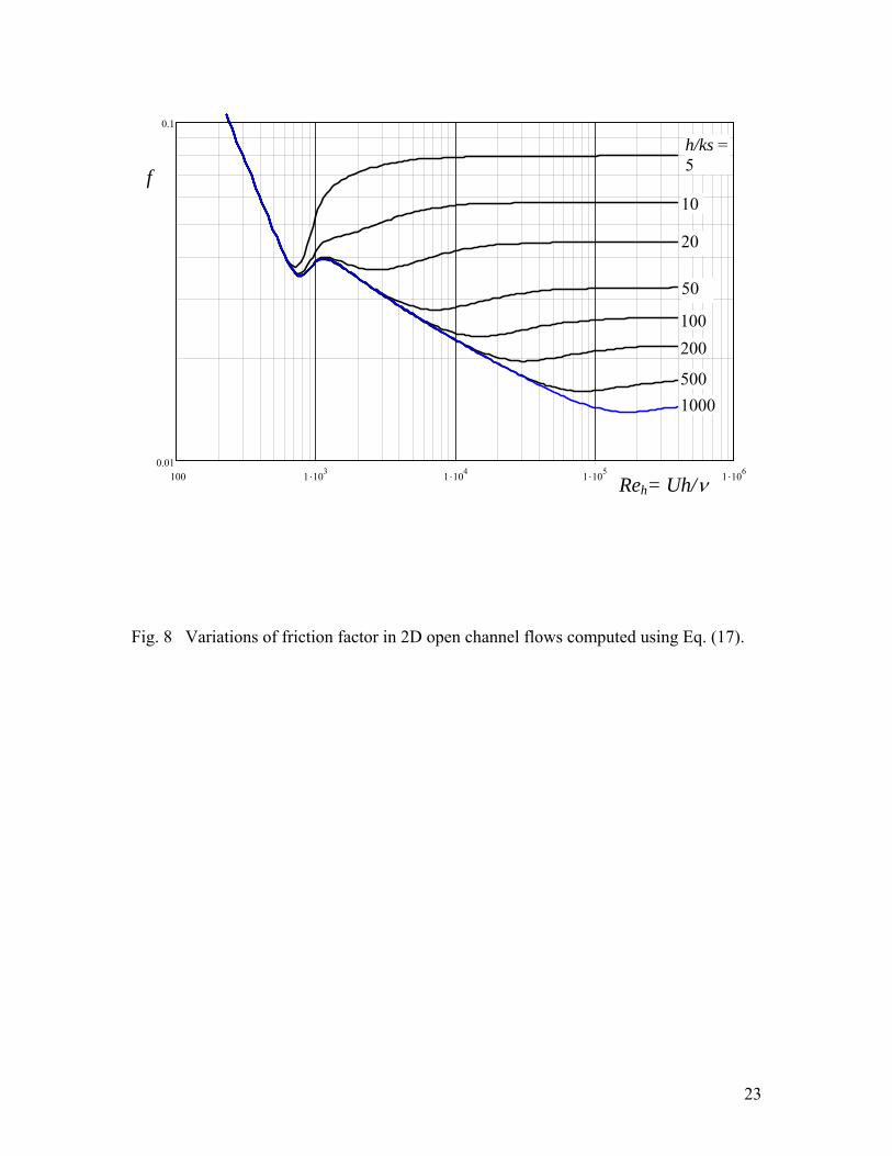
Eq. (17) is applicable for 2D open channel flows over immobile boundaries comprised of

unisized sediment. The variations of f computed using Eq. (17) is plotted in Fig. 8. To

compare Eq. (17) with measurements, a database with wide ranges of Reh and h/ks for

open channel flows, which is similar to that by Nikuradse, is needed but not available at

the current stage. In addition, for open channel flows subject to significant sidewall

12

effects, friction equations similar to Eq. (17) could be also developed with the shape

factor being properly adjusted (Montes 1998). Such studies are worth further efforts.

Conclusions

A useful interpolation function is proposed for computing the friction factor for the two

transitional regimes, one between laminar and turbulent flows and the other between

fully-smooth and fully-rough turbulent flows. The resulted explicit formula represents

well the experimental data by Nikuradse for pipes roughened by well-sorted sand grains,

in comparison with other implicit formulas available in the literature. With the similar

approach, a single explicit equation is also suggested for computing the friction factor in

two-dimensional open channel flows for all flow regimes. It should be mentioned that the

results presented are largely based on Nikuradse’s study, and thus their applications could

be limited.

Notation

The following symbols are used in this note:

b = constant

B = friction factor-related parameter as given by Eq. (12)

D = pipe diameter

E = relative error

13

f = friction factor [f = 8(u*/V)2 for pipe flows; f = 8(u*/U)2 for open channel flows]

fL = friction factor for laminar flows

fT = friction factor for turbulent flows

fTR = friction factor for fully-rough turbulent flows

fTS = friction factor for fully-smooth turbulent flows

h = flow depth

ks = roughness size that is taken as the sand grain diameter for Nikuradse’s

experiments

ks+ = u*ks/ν

m = exponent

n = exponent

Re = Reynolds number for pipe flows (=VD/ν)

ReLT = intermediate Reynolds number in the laminar-turbulent flow transition

ReSR = intermediate Reynolds number in the fully smooth to fully rough turbulent flow

transition

Reh = Reynolds number for open channel flows (=Uh/ν)

r = pipe radius

U = depth-averaged velocity in open channel flows

u = longitudinal flow velocity

u* = friction velocity

14

V = cross-sectional average velocity

y = wall-normal distance

α = weighting factor

β = weighting factor

ν = fluid viscosity

η = constant

References

Barr, D. I. H. (1977). "Discussion of 'Accurate explicit equation for friction factor'."

Journal of Hydraulics Division-ASCE, 103(HY3), 334-337.

Bradshaw, P. (2000). "A note on 'critical roughness height' and 'transitional roughness'."

Physics of Fluids, 12(6), 1611-1614.

Brownlie, W. R. (1981). "Reexamination of Nikuradse roughness data." Journal of the

Hydraulics Division-ASCE, 107(1), 115-119.

Cheng, N. S., and Chiew, Y. M. (1998). "Modified logarithmic law for velocity

distribution subjected to upward seepage." Journal of Hydraulic Engineering-

ASCE, 124(12), 1235-1241.

Colebrook, C. F. (1939). "Turbulent flow in pipes with particular reference to the

transition region between the smooth and rough pipe laws." Proceedings of the

Institution of Civil Engineers, 12, 393-422.

Haaland, S. E. (1983). "Simple and explicit formulas for the friction factor in turbulent

pipe-flow." Journal of Fluids Engineering-Transactions of the ASME, 105(1), 89-

90.

Hinze, J. O. (1975). Turbulence, McGraw-Hill, New York.

Jimenez, J. (2004). "Turbulent flows over rough walls." Annual Review of Fluid

Mechanics, 36, 173-196.

15

Ligrani, P. M., and Moffat, R. J. (1986). "Structure of Transitionally Rough and Fully

Rough Turbulent Boundary-Layers." Journal of Fluid Mechanics, 162, 69-98.

Montes, S. (1998). Hydraulics of open channel flow, ASCE Press, Reston, VA.

Nikuradse, J. (1933). "Stromungsgesetze in rauhen Rohren." Forschung auf dem Gebiete

des Ingenieurwesens, Forschungsheft 361. VDI Verlag, Berlin, Germany (in

German). (English translation: Laws of flow in rough pipes, NACA TM 1292,

1950).

Schlichting, H. (1979). Boundary-layer theory, McGraw-Hill, New York.

Swamee, P. K., and Jain, A. K. (1976). "Explicit equations for pipe-flow problems."

Journal of Hydraulics Division-ASCE, 102(HY5), 657-664.

White, F. M. (1991). Viscous fluid flow, McGraw-Hill, New York.

Yalin, M. S., and Da Silva, A. M. A. F. (2001). Fluvial processes, IAHR, Delft,

Netherlands.

Yen, B. C. (2002). "Open channel flow resistance." Journal of Hydraulic Engineering-

ASCE, 128(1), 20-39.

16

0 1000 2000 3000 4000 5000 6000 7000 8000 9000 1 .1040.01

0.03

0.05

0.07

0.09

0.11

0.13Nikuradse's dataEq. (8)Eq. (5)Eq. (7)Eq. (4)

Fig. 1 Transition between laminar and fully-smooth turbulent flows. The data are

extracted from Tables 2-7 (for ks+ < 5) and Fig. 9 of Nikuradse (1933).

f

Re

17

0 100 200 300 400 500 6000

2 .104

4 .104

6 .104

8 .104

1 .105

1.2 .105

Fig. 2 Relation of ReSR to r/ks

r/ks

ReSR

18

1 .103 1 .104 1 .105 1 .106 1 .1070.01

0.02

0.03

0.04

0.05

0.06

0.07

Fig. 3 Comparison of Eq. (8) with measurements for turbulent pipe flows. The data are

extracted from Tables 2-7 of Nikuradse (1933).

r/ks = 15

30.6

60

126 252 507

fT

Re

19

100 1 .103 1 .104 1 .105 1 .106 1 .1070.01

0.1

Fig. 4 Comparison of Eq. (8) with experimental measurements for laminar and

turbulent pipe flows. The data points are plotted based on Tables 2-7 and Figure 9 of

Nikuradse (1933).

r/ks = 15

30.6

60

126

252

507

f

Re

20

0 0.5 1 1.5 2 2.5 3 3.5 4

6

7

8

9

10

11

r/ks = 15 30.6 60 126 252 507Brownlie (1981)Ligrani & Moffat (1986) Cheng & Chiew (1998) Yalin & Da Silva (2001)

0.5 1 1.5 28

9

10

Fig. 5 Variation of B with ks+. The inset highlights that B is also subject to r/ks in the

transition between fully-smooth and fully-rough regimes. The data plotted are those calculated using Tables 2-7 of Nikuradse (1933) for turbulent pipe flows.

log ks+

B

21

0 0.5 1 1.5 2 2.5 35

6

7

8

9

10

r/ks = 15 30.6 60 126 252 507

Fig. 6 Effect of r/ks on the relation of B-ks+. The curves are computed using Eqs. (8) and

(12) for Re > 5000.

log ks+

B

22

5 10 15 20 25 30 35 40 45 50 55 60 65 700

0.010.020.030.040.050.060.07

5 10 15 20 25 30 35 40 45 50 55 60 65 700

0.010.020.030.040.050.060.07

5 10 15 20 25 30 35 40 45 50 55 60 65 700

0.010.020.030.040.050.060.07

5 10 15 20 25 30 35 40 45 50 55 60 65 700

0.010.020.030.040.050.060.07

Fig. 7 Relative errors in B-values computed from the previous formulas (denoted by

circles) and present formula (denoted by solid lines). E = |Bcalculated - Bmeasured|/Bmeasured.

E

ks+

Lagrani & Moffat (1986)

Cheng & Chiew (1998)

Yalin & Da Silva (2001)

Brownlie (1981)

23

100 1 .103 1 .104 1 .105 1 .1060.01

0.1

Fig. 8 Variations of friction factor in 2D open channel flows computed using Eq. (17).

h/ks =5

10

20

50

100 200

f

Reh= Uh/ν

500 1000