1 Finite Word Length Effects on Transmission Rate in Zero

arX

iv:0

810.

1773

v1 [

cs.IT

] 9

Oct

200

81

Finite Word Length Effects on Transmission

Rate in Zero Forcing Linear Precoding for

Multichannel DSL

Eitan Sayag1,2, Amir Leshem1,3 Senior member, IEEE

and

Nicholas D. Sidiropoulos4 Senior member, IEEE

Abstract

Crosstalk interference is the limiting factor in transmission over copper lines. Crosstalk cancelation

techniques show great potential for enabling the next leap in DSL transmission rates. An important issue

when implementing crosstalk cancelation techniques in hardware is the effect of finite world length on

performance. In this paper we provide an analysis of the performance of linear zero-forcing precoders,

used for crosstalk compensation, in the presence of finite word length errors. We quantify analytically the

trade off between precoder word length and transmission rate degradation. More specifically, we prove

a simple formula for the transmission rate loss as a functionof the number of bits used for precoding,

the signal to noise ratio, and the standard line parameters.We demonstrate, through simulations on

real lines, the accuracy of our estimates. Moreover, our results are stable in the presence of channel

estimation errors. Finally, we show how to use these estimates as a design tool for DSL linear crosstalk

precoders. For example, we show that for standard VDSL2 precoded systems, 14 bits representation of

the precoder entries results in capacity loss below1% for lines over 300m.

Keywords: Multichannel DSL, vectoring, linear precoding, capacity estimates, quantization.

1 School of Engineering, Bar-Ilan University, 52900, Ramat Gan, Israel.2 Dept. of Math. Ben Gurion University, Beer-Sheva,

Israel. 3 Circuit and Systmes, Faculty of EEMCS, Delft University of Technology, Delft, The Netherlands.4 Dept. of ECE,

Technical University of Crete, Greece. This research was partially supported by the EU-FP6 IST, under contract no. 506790,

and by the Israeli ministry of trade and commerce as part of Nehusha\iSMART project. Conference version of part of this work

appeared inProc. IEEE ICASSP 2008, Mar. 30 - Apr. 4, 2008, Las Vegas, Nevada.

October 9, 2008 DRAFT

http://arXiv.org/abs/0810.1773v1

2

I. INTRODUCTION

DSL systems are capable of delivering high data rates over copper lines. A major problem

of DSL technologies is the electromagnetic coupling between the twisted pairs within a binder

group. Reference [1] and the recent experimental studies in[2], [3] have demonstrated that

vectoringandcrosstalk cancelationallow a significant increase of the data rates of DSL systems.

In particular, linear precoding has recently drawn considerable attention [4], [5] as a natural

method for crosstalk precompensation as well as crosstalk cancelation in the receiver. In [2], [3]

it is shown that optimal cancelation achieves capacity boost ranging from2× to 4×, and also

substantially reduces per-loop capacity spread and outage, which are very important metrics from

an operator’s perspective. References [5], [6] advocate the use of a diagonalizing precompensator,

and demonstrate that, without modification of the Customer Premise Equipment (CPE), one can

obtain near optimal performance. Recent work in [7], [8] hasshown that a low-order truncated

series approximation of the inverse channel matrix affordssignificant complexity reduction in the

computation of the precoding matrix. Implementation complexity (i.e., the actual multiplication

of the transmitted symbol vector by the precoding matrix) remains high, however, especially

for multicarrier transmission which requires one matrix-vector multiplication for each tone.

Current advanced DSL systems use thousands of tones. In these conditions, using minimal word

length in representing the precoder matrix is important. However, using coarse quantization

will result in substantial rate loss. The number of quantization bits per matrix coefficient is

an important parameter that affects the system’s performance - complexity trade-off, which we

focus on in this paper. We provide closed form sharp analyticbounds on the absolute and

relative transmission rate loss. We show that both absoluteand relative transmission loss decay

exponentially as a function of the number of quantizer bits and provide explicit bounds for the

loss in each tone. Under analytic channel models as in [9], [10] we provide refined and explicit

bounds for the transmission loss across the band and comparethese to simulation results. This

explicit relationship between the number of quantizer bitsand the transmission rate loss due to

quantization is a very useful tool in the design of practicalsystems.

The structure of the paper is as follows. In section II, we present the signal model for a

precoded discrete multichannel system and provide a model for the precoder errors we study.

In section III, a general formula for the transmission loss of a single user is derived. In section


3

IV we focus on the case of full channel state information where the rate loss of a single user

results from quantization errors only. Here we prove the main result of the paper, Theorem 4.1.

We provide explicit bounds on the rate loss under an analyticmodel for the transfer function as

in [9]. We also study a number of natural design criteria. In section V we provide simulation

results on measured lines, which support our analysis. Moreover, we show through simulation

that our results are valid in the presence of measurement errors. The appendices provide full

details of the mathematical claims used in the main text.

II. PROBLEM FORMULATION

A. Signal model

In this section we describe the signal model for a precoded discrete multitone (DMT) system.

We assume that the transmission scheme is Frequency Division Duplexing (FDD), where the

upstream and the downstream transmissions are performed atseparate frequency bands. More-

over, we assume that all modems are synchronized. Hence, theecho signal is eliminated, as in

[1], and the received signal model at frequencyf is given by

x(f) = H(f)s(f) + n(f), (1)

wheres(f) is the vectored signal sent by the optical network unit (ONU), H(f) is ap×p matrix

representing the channels,n(f) is additive Gaussian noise, andx(f) (conceptually) collects the

signals received by the individual users. The users estimate rows of the channel matrixH(f),

and the ONU uses this information to sendP(f)s(f) instead ofs(f). This process is called

crosstalk pre-compensation. In general such a mechanism yields

x(f) = H(f)P(f)s(f) + n(f). (2)

Denote the diagonal ofH(f) by D(f) = diag(H(f)) and letP(f) = H(f)−1D(f) as suggested

in [5]. With this we have

x(f) = D(f)s(f) + n(f), (3)

showing that the crosstalk is eliminated. Note that withF(f) = H(f) − D(f) we have the

following formula for the matrixP(f)

P(f) =(

I + D−1(f)F(f))−1

. (4)


4

Following [5] we assume that the matricesH(f) are row-wise diagonally dominant, namely that

‖hii‖ >> ‖hij‖, ∀i 6= j. (5)

In fact, motivated in part by Gersgorin’s theorem [11] we propose the parameterr(H)

r(H) = max1≤i≤N

(

∑

j 6=i |hij ||hii|

)

, (6)

as a measure for the dominance. In most downstream scenariosthe parameterr is indeed much

smaller than 1. We emphasize that typical downstream VDSL channels are row-wise diagonally

dominant even in mixed length scenarios as demonstrated in [8].

B. A model for precoder errors

In practical implementations, the entries of the precodingmatrix P will be quantized. The

number of quantizer bits used is dictated by complexity and memory considerations. Indeed,

relatively coarse quantization of the entries of the precoder P allows significant reduction of the

time complexity and the amount of memory needed for the precoding process. The key problem

is to determine the transmission rate loss of an individual user caused by such quantization.

Another closely related problem is the issue of robustness of linear precoding with respect to

errors in the estimation of the channel matrix. The mathematical setting for both is that of error

analysis. Let

P = (I + D−1F + E1)−1 + E2, (7)

where

• E1 models therelative error in quantizing or measuringthe channel matrixH, and

• E2 models theerrors caused by quantizingthe precoderP.

The problem is to determine the capacity of the system, and the capacity of each user, in terms of

the system parameters and the statistical parameters of theerrors. Note that equation (7) captures

three types of errors: errors in the estimation ofH, quantization errors in the representation of

H, and quantization errors in the representation of the precoder P.

Our focus will be in the study of the effect of quantization errors in the representation of the

precoder on the capacity of an individual user. Nevertheless, the estimation errors resulting from

measuring the channel cannot be ignored. We will show that the analysis of quantization errors

and estimation errors can be dealt separately (see remark 3.2 after lemma 3.1). This allows


5

us to carry analysis under the assumption of perfect channelinformation. Then, we show in

simulations that when the estimation errors in channel measurements are reasonably small, our

analytical bounds remain valid.

C. System Model

We now list our assumptions regarding the errorsE1, E2, the power spectral density of the

users, and the behavior of the channel matrices.

Perfect CSI: Perfect Channel Information. Namely,

E1(f) = 0, ∀f. (8)

Quant(2−d): The quantization error of each matrix element of the precoder is at most2−d.

Namely,

|E2(f)i,j| ≤ 2−d, ∀f, ∀i, j. (9)

DD: The channel matrices are row-wise diagonally dominant.

r(H(f)) ≤ 1, ∀f. (10)

SPSD: The Power Spectral Density (PSD) of all the users of the binder is the same. Namely,

we assume that for some fixed unspecified functionP (f) we have:

Pi(f) = P (f), ∀i. (11)

The main result of the paper, Theorem 4.1 is based on assumptions (8), (9), (10), (11).

AssumptionSPSD can be lifted, as shown in section XIV (appendix H). For the sake of clarity

we present only the simplified result in the body of the paper.

In order to obtain sharp analytic estimates on the transmission loss in actual DSL scenarios

we need to incorporate some of the properties of the channel matrices of DSL channels into our

model. In particular, we will assume

Werner Channel model: The matrix elements of the channel matricesH(f) behave as in the

model of [9]. Namely, following [9] we assume the following model for insertion loss

|HIL(f, ℓ)|2 = e−2αℓ√

f (12)


6

whereℓ is the DSL loop length (in meters),f is the frequency in Hz, andα is a parameter that

depends on the cable type. Furthermore, crosstalk is modeled as

|HFEXT (f, ℓ)|2 = K(ℓ)f 2|HIL(f, ℓ)|2 (13)

Here K(ℓ) is a random variable studied in [10]. The finding is thatK(ℓ) is a log-normal

distribution with expectation, denote therec1(ℓ), that increase linearly withℓ.

An additional assumption that we will make concerns the behavior of the row dominance of

the channel matricesH(f, ℓ).

Sub linear row dominance:

r(H(f, ℓ)) ≤ γ1(ℓ) + γ2(ℓ)f (14)

Whereγ2(ℓ) = O(√

ℓ).

Remark 2.1:Note that|HFEXT (ℓ, f)||HIL(f, ℓ)|

=√

K(ℓ)f.

The sub-linearity inf follows by studyingr(H(ℓ, f)) in terms ofp2 random variables behaving

asK(ℓ).

D. Justification of the assumptions

Perfect CSI is plausible due to the quasi-stationarity of DSL systems (long coherence time),

which allows us to estimate the channel matrices at high precision.

Quant(2−d) is a weak assumption on the type of the quantization process.Informally it is

equivalent to an assumption on the number of bits used to quantize an entry in the channel matrix.

In particular, our analysis of the capacity loss will be independent of the specific quantization

method and our results are valid for any technique that quantizes matrix elements with bounded

errors.

AssumptionDD reflects the diagonal dominance of DSL channels. While linear precoding

may result in power fluctuations, the diagonal dominance property of DSL channel matrices

makes these fluctuations negligible within 3.5dB fluctuation allowed by PSD template (G993.2).

For example if the row dominance is up to 0.1 the effect of precoding on the transmit powers

and spectra will be at most 1dB.


7

AssumptionSPSD (see (11)) is justified in a system with ideal full-binder precoding, where

each user will use the entire PSD mask allowed by regulation.Note that in [3] it is shown that

DSM3 provides significant capacity gains only when almost all pairs in a binder are coordinated.

Thus the equal transmit spectra assumption is reasonable inthese systems. However we also

provide in section XIV (appendix H) a generalization of the main result to a setting in which

this assumption is not satisfied.

AssumptionWerner Channel model does not need justification whereas our last assumption,

sub-linear row dominance was verified on measured lines [3] and can also be deduced analyt-

ically from Werner’s model. In practice, the type of fitting required to obtainγ1(ℓ), γ2(ℓ) from

measured data is simple and can be done efficiently. Moreover, the line parameters tabulated

in standard (e.g., R,L,C,G parameters of the two port model), together with the99% worst

case power sum model used in standards [12], provide anotherway of computing the constants

γ1(ℓ), γ2(ℓ).

III. A G ENERAL FORMULA FOR TRANSMISSION LOSS

The purpose of this section is to provide a general formula for the transmission rate loss

of a single user, resulting from errors in the estimated channel matrix as well as errors in the

precoder matrix. First, we develop a useful expression for the equivalent channel in the presence

of errors. This is given in formula (17). Next, a formula for the transmission loss is obtained

(30). The formula compares the achievable rate of a communication system using an ideal ZF

precoder as in (4) versus that of a communication system whose precoder is given by (7). This

formula is the key to the whole paper. Note that we use a gap analysis as in [13], [14]. A useful

corollary in the form of formula (34) is derived. This will beused in the next section to obtain

bounds on capacity loss due to quantization.

Let H(f) = D(f) + F(f) be a decomposition of the channel matrix at a given frequencyto

diagonal and non-diagonal terms. ThusD(f) is a diagonal matrix whose diagonal is identical to

the diagonal ofH(f). Also we letSNRi(f) be the signal to noise ratio of thei-th receiver at

frequencyf

SNRi(f) =Pi(f)|di,i(f)|2

E|ni(f)|2 . (15)

In this formulaPi(f) is the power spectral density (PSD) of thei-th user at frequencyf , and


8

ni(f) is the associated noise term. We denote

σ2ni

(f) = E|ni(f)|2. (16)

A. A formula for the equivalent channel in the presence of errors

We first derive a general formula for the equivalent signal model. The next lemma provides

a useful reformulation of the signal model in (2):

Lemma 3.1:The precoded channel (2) with precoder as in (7) is given by

x(f) = D(f)s(f) + D(f)∆(f)s(f) + n(f), (17)

with

∆(f) = (I + D−1(f)F(f))E2(f) − E1(f)(I + D−1(f)F(f) + E1(f))−1. (18)

The proof is deferred to appendix A (section VII).

Remark 3.2:For our analysis, we will assume thatE1(f) = 0, in which case the formula for

the matrix∆ simplifies to

∆(f) = (I + D−1(f)F(f))E2(f). (19)

The relevance of the formula (18) for the experimental part of the paper (whereE1(f) is not

assumed to be zero) is explained in the next remark.

Remark 3.3:In formula (30) below we show that the impact of the errorsE1(f) and E2(f)

on the transmission loss of a user can be computed from the matrix ∆. Thus, an important

consequence of the lemma is that the effect on transmission loss due to estimation errors (encoded

in the matrixE1(f)) and due to quantization errors (encoded in the matrixE2(f)) can be studied

separately as they contribute to different terms in the above expression for∆.

B. Transmission Loss of a Single User

Consider a communication system as defined in (3) and denote by B the frequency band of

the system. We letSNRi(f) be as in (15) and letΓ be the Shannon Gap comprising modulation

loss, coding gain and noise margin. LetRi be the achievable transmission rate of thei-th user

in the system defined in (3). Recall that in such a system the crosstalk is completely removed

and therefore

Ri =

∫

f∈B

log2(1 + Γ−1SNRi(f))df. (20)


9

Let

Ri(f) = log2(1 + Γ−1SNRi(f)) (21)

be the transmission rate at frequencyf (formally, it is just the density of that rate). LetRi(f)

be the transmission rate at frequencyf of the i-th user, when the precoder in (7) is used. We

note that whileRi(f) is a number, the quantityRi(f) depends on the random variablesE1,E2

and hence is itself a random variable. LetRi be the transmission rate of thei-th user for the

equivalent system in (17). Thus,

Ri =

∫

f∈B

Ri(f)df. (22)

By equation (17), thei-th user receives

xi(f) = di,i(f)si(f) + di,i

p∑

j=1

∆i,j(f)sj(f) + ni(f) = di,i(f)(1 + ∆i,i(f))si(f) + Ni(f) (23)

whereNi(f) = di,i(f)∑p

j 6=i ∆i,j(f)sj(f)+ni(f). Assuming Gaussian signaling i.e. that allsi(f)

are Gaussian we conclude thatNi(f) is Gaussian. A similar conclusion is valid in the case of a

large number of users, due to the Central Limit Theorem. In practice, the Gaussian assumption

is a good approximation even for a modest number of (e.g., 8) users. Recall also that Gaussian

signaling is the optimal strategy in the case of exact channel knowledge. Therefore, we can use

the capacity formula for the Gaussian channel, even under precoder quantization errors.

Definition 3.1: The transmission lossLi(f) of the i-th user at frequencyf is given by

Li(f) = Ri(f) − Ri(f). (24)

The total loss of the i-th user is

Li =

∫

f∈B

Li(f)df. (25)

We are ready to deduce a formula for the rate loss of thei-th user as a result of the non-ideal

precoder in (17). Our result will be given in terms of the matrix ∆. Recall that∆ generally

depends on both precoder quantization errorsE2 and estimation errorsE1.

Denote by∆i,j the (i, j)-th element of the matrix∆ and let

δi(f) = Γ∑

j 6=i

Pj(f)

Pi(f)|∆i,j(f)|2. (26)

Let


10

ai(f) = δi(f)Γ−1SNRi(f) =∑

j 6=i

Pj(f)

Pi(f)|∆i,j(f)|2SNRi(f), (27)

qi(∆, f) =|1 + ∆i,i(f)|2

ai(f) + 1, (28)

and

ki(f) =Γ−1SNRi(f)

Γ−1SNRi(f) + 1. (29)

Note thatai(f) and henceqi(∆, f) are independent of the Shannon gapΓ. The next lemma

provides a formula for the exact transmission rate loss due to the errors modeled by the matrices

E1 and E2. The result is stated in terms of quantitiesq(∆, f) and the effective signal to noise

ratio, Γ−1SNRi(f).

Lemma 3.4:Let H(f) be the channel matrix at frequencyf and letE1, E2 be the estimation

and quantization errors, respectively as in (7). LetLi(f) be the loss in transmission rate of the

i-th user defined in (24). Then

Li(∆, f) = − log2 (1 − ki(f)(1 − qi(∆, f))) , (30)

whereqi(∆, f) is given in (28) andki(f) is given in (29).

In particular, if∆i,i(f) = −1 the transmission loss islog2(1+Γ−1SNRi(f)), whereSNRi(f)

is defined in (15). Finally, if∆i,i(f) 6= −1 we have

Li(∆, f) ≤ Max

(

0, log2

(

1

qi(∆, f)

))

(31)

The proof of this lemma is deferred to appendix B (section VIII).

To formulate a useful corollary we introduce the quantities:

Mi(f) = maxj 6=iPj(f)

Pi(f)(32)

ti(f) = max1≤j≤n|∆i,j | (33)

Corollary 3.5: Let H(f) be thep× p channel matrix at frequencyf and letE1(f), E2(f) be

the estimation and quantization errors respectively as in (7). Let Li(f) be the transmission rate

loss of thei-th user defined in (24). Assume thatti(f) < 1. Then

Li(∆, f) ≤ log2

(

1 + (p − 1)Mi(f)t2i (f)SNRi(f)

(1 − ti(f))2

)

(34)


11

Proof: By (27) we have

ai(f) =∑

j 6=i

Pj(f)

Pi(f)|∆i,j(f)|2SNRi(f) ≤ Mi(f)ti(f)2(p − 1)SNRi(f) (35)

1 + ai(f) ≤ 1 + (p − 1)Mi(f)ti(f)2SNRi(f) (36)

Since|∆i,i(f)| ≤ ti(f) we get

|1 + ∆i,i(f)|2 ≥ (1 − ti(f))2 (37)

Thus by (28) we have

1

qi(∆, f)=

ai(f) + 1

|1 + ∆i,i(f)|2 ≤ 1 + (p − 1)Mi(f)t2i (f)SNRi(f)

(1 − ti(f))2(38)

Notice that the right hand side is larger than one and using (31) of the previous lemma the proof

is complete.

Remark 3.6:We note that under simplifying assumptions, such as assumption SPSD (see (11))

the above formula reduces to

Li(∆, f) ≤ log2(1 + (p − 1)t2i (f)SNRi(f)) − 2 log2(1 − ti(f)) (39)

Under the assumptionPerfect CSI, we have∆(f) = (I + D−1(f)F(f))E2(f) and since we

further assumed that the channel matricesH(f) are row-wise diagonally dominant we see that

∆(f) ≈ E2(f). Thus,ti(f) ≈ 2−d and we obtain a bound of the form

Li(∆, f) ≤ log2(1 + (p − 1)SNRi(f)2−2d) − 2 log2(1 − 2−d) (40)

For a statement of a bound of this form see formula (41) of Theorem 4.1 below.

IV. TRANSMISSION RATELOSSRESULTING FROM QUANTIZATION ERRORS IN THE

PRECODER

In the ZF precoder studied earlier we can assume without lossof generality that the entries

are of absolute value less than one. Each of these values is now represented using2d bits (d bits

for the real part andd bits for the imaginary part, not including the sign bit). We first consider

an ideal situation in which we have perfect channel estimation.


12

A. Transmission Loss with Perfect Channel Knowledge

Consider the case whereE1 = 0 and the quantization error is given by an arbitrary matrixE2

with the property that each entry is a complex number with real and imaginary parts bounded in

absolute value by2−d. We will not make any further assumptions about the particular quantization

method employed and we will provide upper bounds for the capacity loss. We do not assume

any specific random model for the values ofE2 because we are interested in obtaining absolute

upper bounds on capacity loss.

The following theorem describes the transmission rate lossresulting from quantization of the

precoder.

Main Theorem 4.1: Let H(f) be the channel matrix ofp twisted pairs at frequencyf , and

r(f) = r(H(f)) as in (6). AssumePerfect CSI (8), Quant(2−d) (9), SPSD (11), and that the

precoderP(f) is quantized usingd ≥ 12

+ log2(1 + r(f)) bits. The transmission rate loss of the

i-th user at frequencyf due to quantization is bounded by

Li(d, f) ≤ log2(1 + γ(d, f)SNRi(f)) − 2 log2(1 − v(f)2−d), (41)

where

γ(d, f) = 2(p − 1)(1 + r(f))22−2d (42)

and

v(f) =√

2(1 + r(f)). (43)

Furthermore, supposed ≥ 12

+ log2(1 + rmax) with

rmax = maxf∈B(r(H(f)). (44)

Then the transmission loss in the bandB is at most∫

f∈B

log2(1 + γ(d)SNRi(f))df − 2|B| log2(1 − (1 + rmax)2−d+0.5), (45)

where|B| is the total bandwidth,

γ(d) = 2(1 + rmax)2(p − 1)2−2d, (46)

The proof of the theorem is deferred to section IX (appendix C).

We now record some useful corollaries of the theorem illustrating its value.


13

Corollary 4.2: The transmission rate lossLi(∆, f), due to quantization of the precoding

matrix by d bits is bounded by:

Li(∆, f) ≤ log2(1 + γ(d, f)SNRi(f)) − 2 log2(1 − v(f)2−d) (47)

whereγ(d, f) = 2(p − 1)(1 + r(f))22−2d and v(f) =√

2(1 + r(f)). If r(f) ≤ 1, a simplified

looser bound is given by

Li(∆, f) ≤ 2−d+3.5 + log2(1 + 8(p − 1)SNRi(f)2−2d) (48)

For the derivation of the first inequality see (91) in sectionIX. The simplified bound is based

on the estimate− log2(1 − z) ≤ 2z valid for 0 ≤ z ≤ 0.5.

The next result is of theoretical value. It describes the asymptotic behavior ofLi(d) for very

larged.

Corollary 4.3: Under the assumptions of the theorem and assuming thatrmax ≤ 1:

Li(d) = O(2−d).

More precisely, we have

Li(d) = θ

(√32

ln(2)2−dB

)

.

Remark 4.4:By definition, f(n) = θ(g(n)) if and only if

limn→∞f(n)

g(n)= 1

We note that for many practical values of the parameters (e.g. SNR(f) = 80dB, d ≤ 20,

p ≤ 100) the first term in formula (45), involving2−2d, is dominant. Since we are interested in

results that have relevance to existing systems we will develop in the next section, and under some

further assumptions (e.g. assumptions (12), (13)), a boundfor Li(d) of the forma12−2d + a22

−d

where the coefficientsa1, a2 are expressible using the system parameters. This is proposition

4.8.

Ensuring bounded transmission loss in each frequency bin

We now turn to study the natural design requirement that the transmission loss caused due to

quantization of precoders should be bounded by a certain fixed quantity, say 0.1bit/sec/Herz/user,

on a per-tone basis. Such a design criterion is examined in the next corollary.

Corollary 4.5: Let t > 0 and letd be an integer with

d ≥ d(t) (49)


14

With

d(t) =

log2(1.25v(f)2t+1/tln(2)) if 2t − 1 ≤ B2

4A

0.5 log2(5(p − 1)(1 + r)2SNRi(f)/tln(2)) otherwise

Then the transmission loss at tonef due to quantization withd bits is at mostt bps/Hz.

Proof: By theorem 4.1, the loss at a tonef is bounded bylog2

(

1 + 2−2du(f)))

− log2((1 −v(f)2−d)2). Whereu(f) = 2(p − 1)(1 + r)2SNRi(f) andv(f) =

√2(1 + r(f)).

Using 1 − 2t ≤ (1 − t)2 we get

Li(d, f) ≤ log2

(

1 + 2−2du(f)))

− log2(1 − 2v(f)2−d).

We will show that the inequality

log2

(

1 + 2−2du(f)

1 − 2v(f)2−d

)

≤ t (50)

is satisfied for anyd ≥ d(t) as in (49) Letz = 2−d so that the inequality (50) is

1 + z2u(f)

1 − 2v(f)z≤ 2t (51)

This yields a quadratic inequality of the form

Az2 + Bz ≤ T (52)

with A = u(f), B = 2t+1v(f) and T = 2t − 1. Using lemma 10.1 (see section X - appendix

D), we see that ifd ≥ d0(t) where

d0(t) =

log2(1.25v(f)2t+1/(2t − 1) if 2t − 1 ≤ B2

4A

0.5 log2(5(p − 1)(1 + r)2SNRi(f)/(2t − 1)) otherwise

ThenLi(d, f) ≤ t. But d0(t) ≤ d(t) because2t − 1 ≥ ln(2)t and the result follows.

Remark 4.6:The qualitative behavior isd(t) ≈ a1− log2(t) for very small values oft whereas

d(t) ≈ a2 − 0.5 log2(t) for larger values oft.

B. Applications of the Main Theorem

We now apply theorem 4.1 to analyze the required quantization level for DSM level 3 precoders

under several design criteria. To that end letRi be the transmission rate of thei-th user (20)

and letLi be the transmission loss of thei-th user as in (24). Therelative transmission lossis

defined by


15

ηi =Li

Ri=

∫

f∈B

Li(f)df/

∫

f∈B

Ri(f)df (53)

The design criteria are

• Absolute/relative transmission loss across the band is bounded.

• Absolute/relative transmission loss for each tone is bounded.

Bound on Absolute Transmission Loss

From now on, we will assume that the transfer function obeys aparametric model as in [9].

Thus we assume (12) and (13).

To bound the absolute transmission loss we estimate the integral in formula (45) of theorem

4.1.

Using the model (12) one can easily see that

SNRi(f) =Pi(f)

σ2ni

(f)e−2αℓ

√f

Moreover, under the assumption (14) we have a linear bound onthe quantityr(H(f, ℓ)) that is,

r(H(f, ℓ)) ≤ γ1(ℓ) + γ2(ℓ)f

Whereγ2)(ℓ) = O(√

ℓ). Putting these together we can estimate the integral occurring in the

bound (45) and the final conclusion in described in theorem 4.8.

The parametersγ1(ℓ), γ2(ℓ) enter our bounds through the following quantity.

ρℓ = (1 + γ1(ℓ))2 + 12(1 + γ1(ℓ))

γ2(ℓ)

(αℓ)2+ 240

(

γ2(ℓ)

(αℓ)2)2

)

(54)

Remark 4.7:The quantityρℓ behaves as1 + Cℓ−3/2 and is close to one forℓ = 300m.

We are now ready to formulate one of the main results of this paper:

Theorem 4.8:Under assumptionsPerfect CSI, Quant(2−d), SPSD, Werner model andsub-

linear row dominance (see (8), (9), (11), (12), (13), (14)) we have

Li(d)

B≤ ξℓ2

−2d + 2−d+3.5 (55)

where

ξℓ =4

ln(2)(p − 1)

P

σ2n

1

α2B

1

ℓ2ρℓ (56)

We provide a proof of this result in section XI(appendix E).


16

Bound on Relative Transmission Loss

The most natural design criterion is to ensure that therelative capacity lossis below a pre-

determined threshold. We will keep our assumption that the insertion loss behaves as in the

model (12), (13).

Let SNRi = Pi

σ2ni

and SNR′i = Pi

σ2ni

e−α√

B be the Signal to Noise ratios of thei-th user at

the lowest and highest frequencies. We also denote bySNR = SNRi

Γand by SNR′

i =SNR′

i

Γ.

Finally, we denote

ci =1

3log2(SNRi) +

2

3log2(SNR′

i) (57)

The next proposition shows thatci provides a lower bound on the spectral efficiency of thei-th

user.

Proposition 4.1:Assume that the attenuation transfer characteristic of thechannel is given by

(12). Then the spectral efficiency is bounded below by

1

BRi ≥ ci (58)

The proof is deferred to section 4.1 (appendix F).

Corollary 4.9: Let ηi(d) be the relative transmission rate loss of thei-th user as in (53).

Assume that the transfer function satisfies (12) and (13). Then

ηi(d) ≤ ζℓ2−2d +

1

ci2−d+3.5 (59)

where

ζℓ =ξℓ

ci=

4

ln(2)(p − 1)

P

σ2n

1

α2B

1

ℓ2

1

ciρℓ. (60)

Proof: This is an immediate consequence of the upper bound on the average lossLi

Band the

lower bound on1BRi.

Ensuring bounded relative transmission loss in the whole band

The next corollary yields an upper bound for the number of quantized bits required to ensure

that the relative loss is below a given threshold.

Corollary 4.10: Let 0 ≤ τ ≤ 1 and letd ≥ d(τ) where

d(τ) =

log2(12

√2

ciτ) if τ ≤ 32

ζℓc2

0.5 log2(2.5ζℓτ

) otherwise

Then the relative transmission loss caused by quantizationwith d bits is at mostτ .

The proof is a simple application of the previous bound on therelative transmission loss and

lemma 10.1 (section X - appendix D).


17

V. SIMULATION RESULTS

To check the quality of the bounds in theorem 4.1 and its corollaries, we compared the

bounds with simulation results, based on measured channels. We have used the results of the

measurement campaign conducted by France Telecom R&D as described in [10]. All experiments

used the band0 − 30 MHz.

Full band

For each experiment, we generated 1000 random precoder quantization error matricesE2(f),

with i.i.d. elements, and independent real and imaginary parts, each uniformly distributed in the

interval [−2−d, 2d]. We add the error matrix to the precoder matrix to generate the quantized

precoder matrix. Repeating this in each frequency we produced a simulation of the quantized

precoded system and computed the resulting channel capacity of each of the 10 users. Then we

computed the relative and absolute capacity loss of each of the users. In each bin we picked the

worst case out of 1000 quantization trials and obtained a quantity we calledmaximal loss. The

quantity maximal loss is a random variable depending on the number of bits used to quantize

the precoder matrices. Each value of this random variable provides a lower bound for the actual

worst case that can occur when the channel matrices are quantized. We compare this lower bound

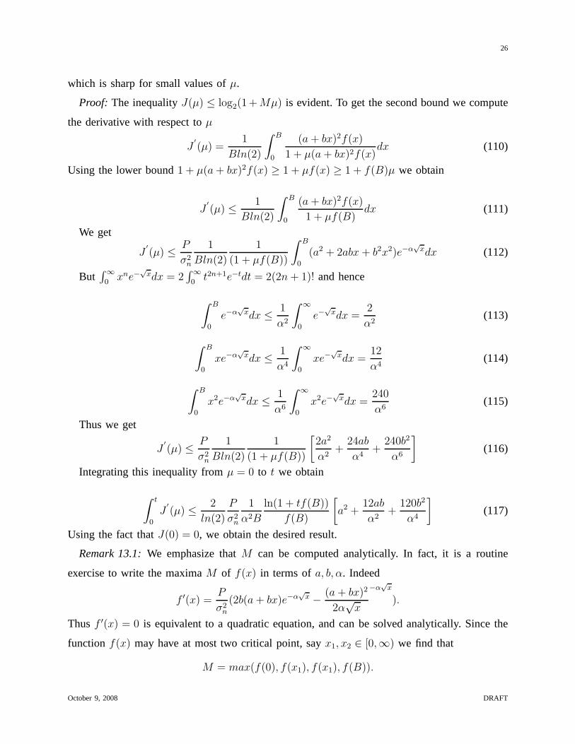
with our upper bounds of theorem 4.1. We have checked our bounds in the following scenario:

Each user has flat PSD of -60dBm/Hz, the noise has flat PSD of -140dBm/Hz. The Shannon

Gap is assumed to be10.7dB. As can be seen in figure 1, the bound given by (45) is sharp. We

also checked the more explicit bound (59) which is based on the model (12), (13). We validated

the linear behavior of the row dominancer(H(f)) as a function of the tonef as predicted by

formula (14). Next we used (12) to fit the parameterα of the cable via the measured insertion

losses. The process of fitting is described in detail in [10].Its value which was used in the bound

(59) wasα = 0.0019. The parametersγ1 = 0.1596 andγ2 = 3.1729 10−8 were estimated from

the measured channel matrices by simple line fit. The resultsare depicted in Figure 1.

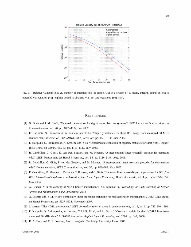
Single frequency

The bounds provided for the entire band are results of boundson each frequency bin. To

show that our bounds are sharp even without averaging over the frequency band, we studied the

capacity loss in specific frequency bins. We concentrated onthe same scenario as before (i.e.


18

with 10 users), the noise is−140dBm/Hz and the power of the users is−60dBm/Hz. We

picked measured matricesH(f1), H(f2), so thatSNR(f1) is 40dBm andSNR(f2) is 60dBm.

As before, we systematically generated an error matrixE2 by choosing its entries to be i.i.d.,

uniformly distributed with maximal absolute value2−d+0.5. Next, we computed the transmission

rate loss using formula (30). By repeating this processN = 10000 times and choosing the worst

event of transmission rate loss, we obtained a lower bound estimate of worst-case transmission

rate loss. This was compared to the bounds of corollary 4.2. The results are depicted in figure

2. Figure 2 uses formula (47). In particular we see that forSNR = 60dB and transmission

rate loss of one percent, simulation indicates quantization with 13 bits. The analytic formula

indicates 14 bits. Similarly, whenSNR = 40dB, and again allowing the same transmission

rate loss of one percent, simulation suggests using 10 bits for quantization. The simple analytic

estimate requires 11 bits.

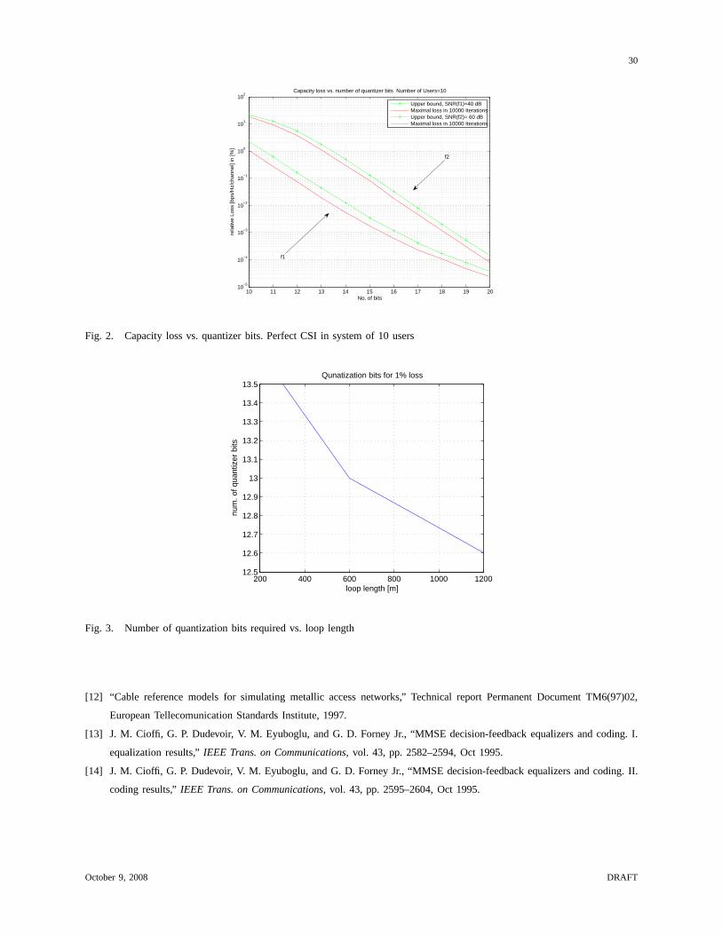
The number of quantizer bits needed to assure 99 percent of capacity

In the next experiment we have studied the number of bits required to obtain a given trans-

mission loss as a function of the loop length. Figure 3 depicts the number of bits required to

ensure transmission rate loss below one percent as a function of loop length. We see that 14

bits are sufficient for loop lengths up to 1200m. Fewer bits are required for longer loops.

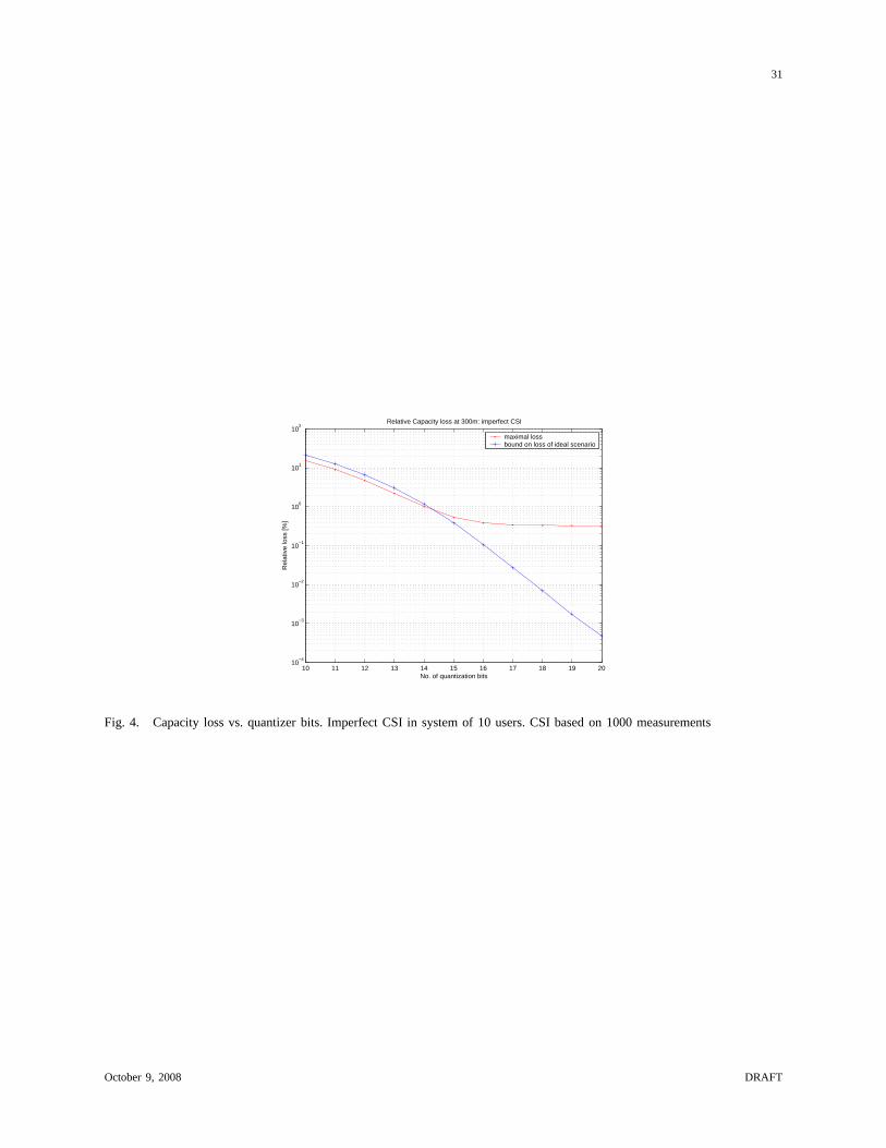
Stability of the results

In the next experiment we validated that the analytic results proven for perfect CSI are valid

even when CSI is imperfect as long as channel measurement errors are not the dominating

cause for capacity loss. To model the measurement errors of the channel matrixH(f), we used

matrices with Gaussian entries with variance which is proportional to SNR(f). More precisely

we assumed that the estimation error of the matrixH(f) is a Gaussian with zero mean and with

varianceσ2H(f)

= 1NSNRi(f)

, whereN is the number of samples used to estimate the channel

matrix H(f). For N = 1000, we estimated the loss in a frequency bin as the worst case outof

500 realizations of quantization noise combined with measurement noise. Figure 3 shows that

as long as the quantization noise is dominant we can safely use our bounds for the transmission

loss. We comment that the stationarity of DSL channels allows accurate channel estimation.


19

VI. CONCLUSIONS

In this paper we analyzed finite word length effects on the achievable rate of vector DSL

systems with zero forcing precoding. The results of this paper provide simple analytic expressions

for the loss due to finite word length. These expressions allow simple optimization of linearly

precoded DSM level 3 systems.

We validated our results using measured channels. Moreover, we showed that our bounds can

be adapted to study the effect of measurement errors on the transmission loss. In practice for

loop lengths between 300 and 1200 meters, one needs 14 bits torepresent the precoder elements

in order to lose no more than one percent of the capacity.

VII. A PPENDIX A: PROOF OFLEMMA 3.1

In this section we prove lemma 3.1.

Proof: For simplicity we will omit the explicit dependency of the matricesH(f), D(f), F(f), P(f)

on the frequencyf . We show that

HP = D + D∆, (61)

with ∆ as above. IndeedH = D(I + D−1F) and thus

HP = D(I + D−1F)((I + D−1F + E1)−1 + E2). (62)

Hence,

HP = D(I + D−1F + E1 − E1)(I + D−1F + E1)−1 + D(I + D−1F)E2. (63)

Thus,

HP = D − DE1(I + D−1F + E1)−1 + D(I + D−1F)E2, (64)

Which proves the lemma.

VIII. A PPENDIX B: PROOF OFLEMMA 3.4

In this appendix we prove lemma 3.4.

Proof: By equation (17), thei-th user receives

xi(f) = di,i(f)si(f) + di,i

p∑

j=1

∆i,j(f)sj(f) + ni(f) = di,i(f)(1 + ∆i,i(f))si(f) + Ni(f) (65)


20

with Ni(f) = di,i(f)∑p

j 6=i ∆i,j(f)sj(f) + ni(f). For a large number of users, we may assume

that Ni(f) is again a Gaussian noise and thetransmission rateat frequencyf of the system

described by equation (65) will be

Ri(∆, f) = log2

(

1 +Pi(f)|di,i(f)|2|(1 + ∆i,i(f))|2

Γ(∑

j 6=i Pj(f)|di,i(f)|2|∆i,j(f)|2 + |ni(f)|2)

)

(66)

Note that this quantity appeared in the main body of the paperjust after equation (22) where it

was denotedRi(f). Dividing both the numerator and denominator byPi(f)|di,i(f)|2 we get

Ri(∆, f) = log2

1 +|(1 + ∆i,i(f))|2

Γ∑

j 6=iPj(f)

Pi(f)|∆i,j(f)|2 + Γ|ni(f)|2

Pi(f)|di,i(f)|2

(67)

or

Ri(∆, f) = log2

(

1 +|(1 + ∆i,i(f))|2δi(f) + 1

eSNRi(f)

)

(68)

where we have defined

eSNRi(f) =SNRi(f)

Γ=

Pi(f)|di,i(f)|2Γ|ni(f)|2 (69)

and

δi(f) = Γ∑

j 6=i

Pj(f)

Pi(f)|∆i,j(f)|2 (70)

To get the transmission rate loss we denote

eSNRi(∆, f) =|(1 + ∆i,i(f))|2δi(f) + 1

eSNRi(f)

(71)

Notice that

eSNRi(f) = eSNRi(0, f)

By definition (24) we have

Li(∆, f) = Ri(f) − Ri(∆, f) = log2(1 + eSNRi(f)) − log2(1 + eSNRi(∆, f)) (72)

We then have

Li(∆, f) = − log2

(

1 + eSNRi(∆, f)

1 + eSNRi(f)

)

= − log2

(

1 − eSNRi(f) − eSNRi(∆, f)

1 + eSNRi(f)

)

(73)

But

eSNRi(f) − eSNRi(∆, f) = eSNRi(f) − |(1 + ∆i,i(f))|2δi + 1

eSNRi(f)

(74)


21

so

eSNRi(f) − eSNRi(∆, f) =eSNRi(f)δi(f) + 1 − |(1 + ∆i,i(f))|2

δi + 1eSNRi(f)

(75)

and finally,

eSNRi(f) − eSNRi(∆, f) = eSNRi(f)eSNRi(f)δi(f) + 1 − |(1 + ∆i,i(f))|2

δi(f)eSNRi(f) + 1(76)

Hence

Li(∆, f) = − log2

(

1 − eSNRi(f)

eSNRi(f) + 1

ai(f) + 1 − |1 + ∆i,i|2ai(f) + 1

)

(77)

where

ai(f) = δi(f)eSNRi(f) (78)

andδi(f) is given in (70). With the notations (28) and (29) we get the formula

Li(∆, f) = − log2 (1 − ki(f)(1 − qi(∆, f))) (79)

To prove the bound we consider two cases. Whenq(∆, f) > 1 we see from equation (79)

thatLi(∆, f) ≤ 0. This clearly indicates transmission gain and the stated inequality is valid. On

the other hand, ifqi(∆, f) ≤ 1 we get

eSNRi

eSNRi + 1(1 − qi(∆, f)) ≤ 1 − qi(∆, f) (80)

and using the monotonicity of− log2(1 − u) (increasing) in the interval(0, 1), we get

Li(∆, f) ≤ − log2 (1 − (1 − qi(∆, f)))) = log2

(

1

qi(∆, f)

)

(81)

and the Lemma is proved.

IX. A PPENDIX C: PROOF OF THEOREM4.1

For the proof of the theorem we need a simple lemma.

Lemma 9.1:Let A be a complexp × p matrix and defineD to be the diagonal matrix with

Di,i = Ai,i for i = 1, .., p. Let E be ap× p matrix whose entries are complex numbers with real

and imaginary parts bounded by2−d. Finally, let B = D−1AE. Then|Bi,j| ≤ 2−d+1/2(1 + r(A)).

Proof: Let Q = D−1A = I + D−1(A − D). Then we havep∑

k=1

|Qik| ≤ 1 + r(A) (82)


22

for all i = 1, .., p. Therefore

|Bi,j| =

∣

∣

∣

∣

∣

p∑

k=1

QikEkj

∣

∣

∣

∣

∣

≤ 2−d+1/2

p∑

k=1

|Qik| ≤ 2−d+1/2(1 + r) (83)

Proof of the main theorem

We first bound the lossLi(f) in a particular tonef . By Lemma 3.4 we have

Li(∆, f) ≤ Max

(

0, log2

(

1

qi(∆, f)

))

(84)

where

qi(∆, f) =|1 + ∆i,i(f)|2

ai(f) + 1(85)

Here∆(f) = (I + D(f)−1F(f))E2(f) whereH(f) = D(f) + F(f) is the channel matrix at

frequencyf andE2(f) is a matrix whose entries are complex numbers with real and imaginary

parts bounded by2−d. Applying Lemma (9.1) to the matrixH(f) we see that the entries∆i,j(f)

are all in a disk of radiusv(f)2−d around zero. Usingr(f) ≤ 5 we obtainv(f) =√

2(1+r(f)) ≤6√

2. Usingd ≥ 4 we get1 − 2−dv(f) ≥ 1 − 6√

216

> 0.

Thus

|1 + ∆i,i(f)|2 ≥ (1 − v2−d)2. (86)

Using the assumption on the PSD of the different users we obtain

ai(f) =∑

j 6=i

Pj(f)

Pi(f)|∆i,j(f)|2SNRi(f) =

∑

j 6=i

|∆i,j(f)|2SNRi(f). (87)

Using Lemma (9.1) we have

∑

j 6=i

|∆i,j(f)|2 ≤ (p − 1)2−2d+1(1 + r(f))2, (88)

thus,

1 + ai(f) ≤ 1 + (p − 1)2−2d+1(1 + r(f))2SNRi(f) = 1 + γ(d, f)SNRi(f). (89)

Combining (85), (86) and (89) we obtain

1

qi(∆, f)≤ 1 + γ(d, f)SNRi(f)

(1 − v(f)2−d)2(90)


23

Note that the right hand side of the above inequality is positive and greater than one. Combining

(31) and (90) we obtain

Li(∆, f) ≤ log2

(

1 + γ(d, f)SNRi(f)

(1 − v(f)2−d)2

)

= log2(1 + γ(d, f)SNRi(f)) − 2 log2(1 − v(f)2−d)

(91)

Sinceγ(d, f) ≤ 2(1+rmax)2(p−1)2−2d andv(f) =

√2(1+r(f)) ≤

√2(1+rmax), integrating

this inequality overf ∈ B we obtain (45) and the theorem is proved.

X. APPENDIX D: PROOFS OFCOROLLARY 4.8 AND 4.9

A. A Quadratic Inequality

In the proof of corollary 4.8 and corollary 4.9 we use the following lemma.

Lemma 10.1:Let A, B, T be positive real numbers and let

d(T ) =

log2(1.25B/T ) if T ≤ B2

4A

0.5 log2(2.5A/T ) otherwise

Then ford ≥ d(T ) we have

A2−2d + B2−d ≤ T (92)

Proof: We let x = 2−d and observe thatf(x) = Ax2 + Bx is monotone inx > 0 with one

root of f(x) = T exactly atx0 =√

B2+4AT−B2A

. Thus for anyd > d0(T ) = log2(2A√

B2+4AT−B) we

haveA2−2d + B2−d = f(2−d) ≤ f(2−d0) = f(x0) = T. To complete the proof we will show

that d0(T ) ≤ d(T ). Indeed,

d0(T ) = log2

(

2A√B2 + 4AT − B

)

= log2

(

2A(√

B2 + 4AT + B)

4AT

)

(93)

Thus,

d0(T ) = log2

(

B

2T(

√

1 +4AT

B+ 1)

)

(94)

If we let ρ = 4ATB2 then forρ < 1 we have

√1 + ρ + 1 ≤ 2.5 and this yields the bound

d0(T ) ≤ log2

(

1.25B

T

)

(95)

for T ≤ B2

4A. On the other hand ifρ > 1 it is easy to see that1 +

√1 + ρ ≤ 2.5

√ρ thus


24

d0(T ) ≤ log2

(

B

2T(2.5

√

4AT

B2)

)

= log2

(

2.5

√

A

T

)

(96)

Remark 10.2:Note that asT decreases to zero the value ofd(T ) increases and behaves as

log2(1T).

XI. A PPENDIX E: PROOF OF THEOREM4.8

Proof: Using Theorem 4.1, the capacity loss of thei-th user,Li(d), is bounded by

Li(d) ≤∫

f∈B

log2(1 + γ(d, f)P

σ2n

e−αℓ

√f)df − 2|B| log2(1 − 2−d+1.5) (97)

By assumption,γ(d, f) ≤ 2(p − 1)2−2d(1 + γ1 + γ2f)2. To bound the first term we state here a

simple lemma (for the proof see section XIII - appendix G)).

Lemma 11.1:Let f(x) = Pσ2

ne−α

√x and define

Ja,b(µ) =1

B

∫ B

0

log2(1 + µ(a + bx)2f(x))dx (98)

We have

J(µ) ≤ eα√

B

α2B

(

2a2 + 24ab

α2+ 240

( a

α2

)2)

log2 (1 + µf(B)) (99)

We can now finish the proof of the theorem.

Let a = 1 + γ1, b = γ2 andµ = 2(p − 1)2−2d, and letJ = Ja,b as in the lemma above. From

(97) we get

1

BLi(d) ≤ J(2(p − 1)2−2d) − 2 log2(1 − 2−d+1.5) (100)

Using the inequality− log2(1−z) ≤ 2z, for z ≤ 12, and the inequality provided by the lemma

for J(µ) we obtain

1

BLi(d) ≤ eαℓ

√B

α2B

(

2(1 + γ1(ℓ))2 + 24(1 + γ1(ℓ))

γ2(ℓ)

(αℓ)2+ 240

(

γ2(ℓ)

(αℓ)2

)2)

log2(1+2(p−1)2−2df(B))+2−d+3.5

(101)

Using log2(1+ t) ≤ ln(2)t, the fact thatf(B) = Pσ2

ne−α

√B and the definition ofρℓ in (54) we

obtain

1

BLi(d) ≤ 4

ln(2)(p − 1)

P

σ2n

1

(αℓ)2Bρℓ2

−2d + 2−d+3.5 (102)


25

XII. A PPENDIX F: PROOF OF PROPOSITION4.1

Proof: We begin with a bound on the transmission rate of the users. By(20) and the model

(12) we obtain

Ri =

∫

f∈B

log2(1 + Γ−1SNRe−αℓ

√f)df ≥ log2(e)

∫

f∈B

ln(Γ−1SNRe−αℓ

√f )df (103)

Thus,

Ri ≥ B log2(Γ−1SNR) − log2(e)

∫ B

0

αℓ

√

fdf ≥ B log2(Γ−1SNR) − 2

3log2(e)αℓB

√B (104)

We notice that this, withSNR′ = SNRe−αℓ

√B implies

1

BRi ≥ log2(Γ

−1SNR)−2

3log2(e)(ln(SNR)−ln(SNR′)) =

1

3log2(SNR)+

2

3log2(SNR′)−log2(Γ),

(105)

and the proof is complete.

Remark 12.1:In practice, the estimation ofαℓ is more reliable than the measurement of the

transfer function at the edge of the frequency band. Thus, the equivalent form

1

BRi ≥ log2(SNR) − 2

3αℓ

√B (106)

is more reliable.

XIII. A PPENDIX G: PROOF OF LEMMA 11.1

In this section we prove lemma 11.1. Recall

J(µ) =1

B

∫ B

0

log2(1 + µ(a + bx)2f(x))dx (107)

wheref(x) = Pσ2

ne−α

√x

Lemma:Let a ≥ 1 and b ≥ 0. Let M be the maximal value of(a + bx)2f(x) in the interval

[0, B]. We have

J(µ) ≤ min

(

eα√

B

α2B

(

2a2 + 24ab

α2+ 240(

b

α2)2

)

log2 (1 + µf(B)) , log2 (1 + Mµ)

)

(108)

In particular we have

J(µ) ≤ 2P

ln(2)α2Bσ2n

(

a2 + 12ab

α2+ 120

(

b

α2

)2)

µ (109)


26

which is sharp for small values ofµ.

Proof: The inequalityJ(µ) ≤ log2(1+ Mµ) is evident. To get the second bound we compute

the derivative with respect toµ

J′

(µ) =1

Bln(2)

∫ B

0

(a + bx)2f(x)

1 + µ(a + bx)2f(x)dx (110)

Using the lower bound1 + µ(a + bx)2f(x) ≥ 1 + µf(x) ≥ 1 + f(B)µ we obtain

J′

(µ) ≤ 1

Bln(2)

∫ B

0

(a + bx)2f(x)

1 + µf(B)dx (111)

We get

J′

(µ) ≤ P

σ2n

1

Bln(2)

1

(1 + µf(B))

∫ B

0

(a2 + 2abx + b2x2)e−α√

xdx (112)

But∫∞

0xne−

√xdx = 2

∫∞0

t2n+1e−tdt = 2(2n + 1)! and hence

∫ B

0

e−α√

xdx ≤ 1

α2

∫ ∞

0

e−√

xdx =2

α2(113)

∫ B

0

xe−α√

xdx ≤ 1

α4

∫ ∞

0

xe−√

xdx =12

α4(114)

∫ B

0

x2e−α√

xdx ≤ 1

α6

∫ ∞

0

x2e−√

xdx =240

α6(115)

Thus we get

J′

(µ) ≤ P

σ2n

1

Bln(2)

1

(1 + µf(B))

[

2a2

α2+

24ab

α4+

240b2

α6

]

(116)

Integrating this inequality fromµ = 0 to t we obtain

∫ t

0

J′

(µ) ≤ 2

ln(2)

P

σ2n

1

α2B

ln(1 + tf(B))

f(B)

[

a2 +12ab

α2+

120b2

α4

]

(117)

Using the fact thatJ(0) = 0, we obtain the desired result.

Remark 13.1:We emphasize thatM can be computed analytically. In fact, it is a routine

exercise to write the maximaM of f(x) in terms ofa, b, α. Indeed

f ′(x) =P

σ2n

(2b(a + bx)e−α√

x − (a + bx)2

2α√

x

−α√

x

).

Thusf ′(x) = 0 is equivalent to a quadratic equation, and can be solved analytically. Since the

function f(x) may have at most two critical point, sayx1, x2 ∈ [0,∞) we find that

M = max(f(0), f(x1), f(x1), f(B)).


27

XIV. A PPENDIX H: L IFTING THE ASSUMPTION OF EQUALPSDFROM THE MAIN THEOREM

In this appendix we prove a slight generalization of the mainresult, showing that the assump-

tion of equal PSD in the binder is not necessary. The resulting bound is similar to that of the

main theorem 4.1.

To formulate the bound on the transmission loss we introducethe quantities

Pmax(f) = maxi(Pi(f)) (118)

Pmin(f) = mini:Pi(f)6=0(Pi(f)) (119)

We let ρ(f) = Pmax(f)/Pi(f). We will say that the PSD satisfies the assumptionSPSD(ρ)

(or has dynamic range of widthρ) if we have

Pmax(f) ≤ ρPmin(f)

We emphasize that this means that for eachf such thatPi(f) 6= 0 we have

Pmax(f) ≤ ρPi(f)

Remark 14.1:In realistic scenarios the numberρ is limited by the maximal power back-off

parameter of the modems in the system.

Theorem 14.2:Assume assumptionsPerfect CSI, Quant(2−d), and SPSD(ρ). Assume that

the precoderP(f) is quantized usingd ≥ 12

+ log2(1 + rmax)) bits. Let H(f) be the channel

matrix of p twisted pairs at frequencyf . Let r(f) = r(H(f)) as in (6). The transmission rate

loss of thei-th user at frequencyf due to quantization is bounded by

Li(d, f) ≤ log2(1 + γ(d, f)SNRi(f)) − 2 log2(1 − v(f)2−d), (120)

where

γ(d, f) = 2ρ(f)(p − 1)(1 + r(f))22−2d (121)

and

v(f) =√

2(1 + r(f)). (122)

Furthermore, the transmission loss in the bandB is at most∫

f∈B

log2(1 + γ(d)SNRi(f))df − 2|B| log2(1 − (1 + rmax)2−d+0.5), (123)


28

where|B| is the total bandwidth, and

γ(d) = 2ρ(1 + rmax)2(p − 1)2−2d. (124)

Proof: Only few changes in the proof of theorem 4.1 are needed in order to derive the

above theorem. In the proof of the main theorem instead of (87) we have

ai(f) =∑

j 6=i

Pj(f)

Pi(f)|∆i,j(f)|2SNRi(f) ≤

∑

j 6=i

ρ(f)|∆i,j(f)|2SNRi(f). (125)

The bound on∆i,j(f) obtained in (88) is valid because our assumptions on the quantization

are the same as in theorem 4.1. Following the same line of reasoning as in equations (89)-(90)

yields the bound (120). This, together with the assumptionSPSD(ρ) easily yields (123).


29

10 11 12 13 14 15 16 17 1810

−3

10−2

10−1

100

101

102

No. of quantization bits

Rel

ativ

e lo

ss [%

]

Relative Capacity loss at 300m with Perfect CSI

maximal lossintegral bound on lossexplicit bound

Fig. 1. Relative Capacity loss vs. number of quantizer bits in perfect CSI in a system of 10 users. Integral bound on loss is

obtained via equation (45), explicit bound is obtained via (59) and equations (60), (57).

REFERENCES

[1] G. Ginis and J. M. Cioffi, “Vectored transmission for digital subscriber line systems,”IEEE Journal on Selected Areas in

Communications, vol. 20, pp. 1085–1104, Jun 2002.

[2] E. Karipidis, N. Sidiropoulos, A. Leshem, and Y. Li, “Capacity statistics for short DSL loops from measured 30 MHz

channel data,” inProc. of IEEE SPAWC 2005, NYC, NY, pp. 156 – 160, June 2005.

[3] E. Karipidis, N. Sidiropoulos, A. Leshem, and Y. Li, “Experimental evaluation of capacity statistics for short VDSLloops,”

IEEE Trans. on Comm., vol. 53, pp. 1119–1122, July 2005.

[4] R. Cendrillon, G. Ginis., E. van Den Bogaert, and M. Moonen, “A near-optimal linear crosstalk canceler for upstream

vdsl,” IEEE Transactions on Signal Processing, vol. 54, pp. 3136–3146, Aug. 2006.

[5] R. Cendrillon, G. Ginis, E. van den Bogaert, and M. Moonen, “A near-optimal linear crosstalk precoder for downstream

vdsl,” Communications, IEEE Transactions on, vol. 55, pp. 860–863, May 2007.

[6] R. Cendrillon, M. Moonen, J. Verlinden, T. Bostoen, and G. Ginis, “Improved linear crosstalk precompensation for DSL,” in

IEEE International Conference on Acoustics, Speech and Signal Processing, Montreal, Canada, vol. 4, pp. IV – 1053–1056,

May 2004.

[7] A. Leshem, “On the capacity of NEXT limited multichannelDSL systems,” inProceedings of IEEE workshop on Sensor

Arrays and Multichannel signal processing, 2004.

[8] A. Leshem and Y. Li, “A low complexity linear precoding technique for next generation multichannel VDSL,”IEEE trans.

on Signal Processing, pp. 5527–5534, November 2007.

[9] J. Werner, “The HDSL environment,”IEEE Journal on selected areas in communications, vol. 9, no. 6, pp. 785–800, 1991.

[10] E. Karipidis, N. Sidiropoulos, A. Leshem, Y. Li, R. Tarafi, and M. Ouzzif, “Crosstalk models for short VDSL2 lines from

measured 30 MHz data,”EURASIP Journal on Applied Signal Processing, vol. 2006, pp. 1–9, 2006.

[11] R. A. Horn and C. R. Johnson,Matrix analysis. Cambridge University Press, 1985.


30

10 11 12 13 14 15 16 17 18 19 2010

−5

10−4

10−3

10−2

10−1

100

101

102

Capacity loss vs. number of quantizer bits Number of Users=10

No. of bits

rela

tive

Loss

[bps

/Hz/

chan

nel]

in [%

]

Upper bound, SNR(f1)=40 dBMaximal loss in 10000 IterationsUpper bound, SNR(f2)= 60 dBMaximal loss in 10000 Iterations

f1

f2

Fig. 2. Capacity loss vs. quantizer bits. Perfect CSI in system of 10 users

200 400 600 800 1000 120012.5

12.6

12.7

12.8

12.9

13

13.1

13.2

13.3

13.4

13.5

loop length [m]

num

. of q

uant

izer

bits

Qunatization bits for 1% loss

Fig. 3. Number of quantization bits required vs. loop length

[12] “Cable reference models for simulating metallic access networks,” Technical report Permanent Document TM6(97)02,

European Tellecomunication Standards Institute, 1997.

[13] J. M. Cioffi, G. P. Dudevoir, V. M. Eyuboglu, and G. D. Forney Jr., “MMSE decision-feedback equalizers and coding. I.

equalization results,”IEEE Trans. on Communications, vol. 43, pp. 2582–2594, Oct 1995.

[14] J. M. Cioffi, G. P. Dudevoir, V. M. Eyuboglu, and G. D. Forney Jr., “MMSE decision-feedback equalizers and coding. II.

coding results,”IEEE Trans. on Communications, vol. 43, pp. 2595–2604, Oct 1995.


31

10 11 12 13 14 15 16 17 18 19 2010

−4

10−3

10−2

10−1

100

101

102

No. of quantization bits

Rel

ativ

e lo

ss [%

]

Relative Capacity loss at 300m: imperfect CSI

maximal lossbound on loss of ideal scenario

Fig. 4. Capacity loss vs. quantizer bits. Imperfect CSI in system of 10 users. CSI based on 1000 measurements


Documents

1 Finite Word Length Effects on Transmission Rate in Zero