Embed Size (px)
Citation preview

1
Fin650:Project Appraisal
Lecture 5
Project Appraisal Under Uncertainty and Appraising Projects with Real Options

Activity Schedule: FIN650Class Date Exams Paper
1 1 June
2 8 June
3 15 June
4 22 June Mid 1
5 20 July
6 27 July Lab Class
7 3 August Lab Class
8 17 August
9 24 August
10 31 August Mid 2
11 2 September (Mon)
12 TBA Paper 2
Originally scheduled classes Makeup classes (Announced by University) Makeup classes proposed (To be finalized in consultation with students)

3
Project Analysis Under Risk
Incorporating risk into project analysis through adjustments to the discount rate, and by the certainty equivalent factor.

4
Introduction: What is Risk? Risk is the variation of future
expectations around an expected value.
Risk is measured as the range of variation around an expected value.
Risk and uncertainty are interchangeable words.

5
Where Does Risk Occur? In project analysis, risk is the
variation in predicted future cash flows.
End of End of End of End of Year 0 Year 1 Year 2 Year 3
-$760 ? -$876 ? -$546 ?-$235 ? -$231 ? -$231 ?
-$1,257 $127 ? $186 ? $190 ?$489 ? $875 ? $327 ?$945 ? $984 ? $454 ?
Varying Cash FlowsForecast Estimates of

6
Handling Risk
Risk may be accounted for by evaluating the project using sensitivity and breakeven analysis.
Risk may be accounted for by (1) applying a discount rate commensurate with the riskiness of the cash flows, and (2), by using a certainty equivalent factor
There are several approaches to handling risk:
Risk may be accounted for by evaluating the project under simulated cash flow and discount rate scenarios.

7
Using a Risk Adjusted Discount Rate The structure of the cash flow
discounting mechanism for risk is:-
The $ amount used for a ‘risky cash flow’ is the expected dollar value for that time period.
A ‘risk adjusted rate’ is a discount rate calculated to include a risk premium. This rate is known as the RADR, the Risk Adjusted Discount Rate.

8
Defining a Risk Adjusted Discount Rate
Conceptually, a risk adjusted discount rate, k, has three components:-
1. A risk-free rate (r), to account for the time value of money
2. An average risk premium (u), to account for the firm’s business risk
3. An additional risk factor (a) , with a positive, zero, or negative value, to account for the risk differential between the project’s risk and the firms’ business risk.

9
Calculating a Risk Adjusted Discount RateA risky discount rate is conceptually definedas:
k = r + u + a
Unfortunately, k, is not easy to estimate. Two approaches to this problem are:
1. Use the firm’s overall Weighted Average Cost of Capital, after tax, as k . The WACC is the overall rate of return required to satisfy all suppliers of capital.
2. A rate estimating (r + u) is obtained from the Capital Asset Pricing Model, and then a is added.

10
Calculating the WACC
Assume a firm has a capital structure of:50% common stock, 10% preferred stock, 40% long term debt.
Rates of return required by the holders of each are :common, 10%; preferred, 8%; pre-tax debt, 7%. The firm’s income tax rate is 30%.
WACC = (0.5 x 0.10) + (0.10 x 0.08) + (0.40 x (0.07x (1-0.30))) = 7.76% pa, after tax.

11
The Capital Asset Pricing Model This model establishes the covariance
between market returns and returns on a single security.
The covariance measure can be used to establish the risky rate of return, r, for a particular security, given expected market returns and the expected risk free rate.

12
Calculating r from the CAPM
The equation to calculate r, for a security with a calculated Beta is:
Where : is the required rate of return being calculated, is the risk free rate: is the Beta of the security, and is the expected return on the market.
rE ~fR
mR

13
Beta is the Slope of an Ordinary Least Squares Regression Line
Share Returns Regressed On Market Returns
-0.04
-0.02
0.00
0.02
0.04
0.06
0.08
0.10
0.12
-0.10 -0.05 0.00 0.05 0.10 0.15 0.20
Returns on Market, % pa
Ret
urn
s o
f S
har
e, %
p
a

14
The Regression Process
The value of Beta can be estimated as the regression coefficient of a simple regression model. The regression coefficient ‘a’ represents the intercept on the y-axis, and ‘b’ represents Beta, the slope of the regression line.
itmtiit urbar
Where, = rate of return on individual firm i’s shares at time t = rate of return on market portfolio at time t = random error term (as defined in regression
analysis)
mtruit

15
The Certainty Equivalent Method: Adjusting the cash flows to their ‘certain’ equivalents
The Certainty Equivalent method adjusts the cash flows for risk, and then discounts these ‘certain’ cash flows at the risk free rate.
COetc
r
bCF
r
bCFNPV
22
11
11
Where: b is the ‘certainty coefficient’ (established by management, and is between 0 and 1); and r is the risk free rate.

16
Analysis Under Risk :Summary
Risk is the variation in future cash flows around a central expected value.
Risk can be accounted for by adjusting the NPV calculation discount rate: there are two methods – either the WACC, or the CAPM
Risk can also be accommodated via the Certainty Equivalent Method.
All methods require management judgment and experience.

17
Appraising Projects with Real Options•Critics of the DCF criteria argue that cash flow analysis fails to account for flexibility in business decisions.•Real option models are more focused on describing uncertainty and in particular the managerial flexibility inherent in many investments•Real options give the firm the opportunity but not the obligation to take certain action

18
What is Options? In finance, an option is a derivative financial instrument that
specifies a contract between two parties for a future transaction on an asset at a reference price. The buyer of the option gains the right, but not the obligation, to engage in that transaction, while the seller incurs the corresponding obligation to fulfill the transaction. The price of an option derives from the difference between the reference price and the value of the underlying asset (commonly a stock, a bond, a currency or a futures contract) plus a premium based on the time remaining until the expiration of the option. Other types of options exist, and options can in principle be created for any type of valuable asset.
An option which conveys the right to buy something is called a call; an option which conveys the right to sell is called a put. The reference price at which the underlying may be traded is called the strike price or exercise price. The process of activating an option and thereby trading the underlying at the agreed-upon price is referred to as exercising it it. Most options have an expiration date. If the option is not exercised by the expiration date, it becomes void and worthless.

19
What is Real Options? Application of financial options theory to
investment in a non-financial (real) asset Hence the name real options

20
Real Options: Link between Investments and Black-Scholes Inputs

21
Real Options in Capital Projects Ten real options to:
Invest in a future capital project Delay investing in a project Choose the project’s initial capacity Expand capacity of the project subsequent to the
original investment Change the project’s technology Change the use of project during its life Shutdown the project with the intention of restarting it
later Abandon or sell the project Extend the life of the project Invest in further projects contingent on investment in
the initial project

What is a real option? Real options exist when managers can
influence the size and risk of a project’s cash flows by taking different actions during the project’s life in response to changing market conditions.
Alert managers always look for real options in projects.
Smarter managers try to create real options.

It does not obligate its owner to take any action. It merely gives the owner the right to buy or sell an asset.
What is the single most importantcharacteristic of an option?

How are real options different from financial options?
Financial options have an underlying asset that is traded--usually a security like a stock.
A real option has an underlying asset that is not a security--for example a project or a growth opportunity, and it isn’t traded.
(More...)

How are real options different from financial options?
The payoffs for financial options are specified in the contract.
Real options are “found” or created inside of projects. Their payoffs can be varied.

What are some types of real options?
Investment timing options Growth options
Expansion of existing product line New products New geographic markets

Types of real options (Continued)
Abandonment options Contraction Temporary suspension
Flexibility options

Five Procedures for ValuingReal Options
1. DCF analysis of expected cash flows, ignoring the option.
2. Qualitative assessment of the real option’s value.
3. Decision tree analysis.
4. Standard model for a corresponding financial option.
5. Financial engineering techniques.

Analysis of a Real Option: Basic Project
Initial cost = $70 million, Cost of Capital = 10%, risk-free rate = 6%, cash flows occur for 3 years.
AnnualDemand Probability Cash Flow
High 30% $45Average 40% $30Low 30% $15

Approach 1: DCF Analysis E(CF) =.3($45)+.4($30)+.3($15)
= $30. PV of expected CFs = ($30/1.1) +
($30/1.12) + ($30/1.13) = $74.61 million. Expected NPV = $74.61 - $70
= $4.61 million
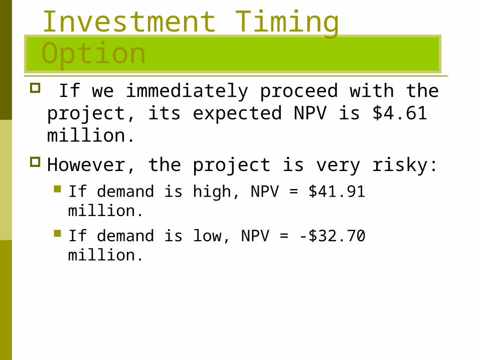
Investment Timing Option If we immediately proceed with the
project, its expected NPV is $4.61 million. However, the project is very risky:
If demand is high, NPV = $41.91 million. If demand is low, NPV = -$32.70 million.

Investment Timing (Continued)
If we wait one year, we will gain additional information regarding demand.
If demand is low, we won’t implement project.
If we wait, the up-front cost and cash flows will stay the same, except they will be shifted ahead by a year.

Procedure 2: Qualitative Assessment
The value of any real option increases if: the underlying project is very risky there is a long time before you must exercise
the option This project is risky and has one year
before we must decide, so the option to wait is probably valuable.

Decision Tree Analysis(Implement only if demand is not low.)
NPV thisCost
0 Prob. 1 2 3 4 Scenarioa
-$70 $45 $45 $4530%
$0 40% -$70 $30 $30 $3030%
$0 $0 $0 $0
Future Cash Flows
Discount the cost of the project at the risk-free rate, since the cost is known. Discount the operating cash flows at the cost of capital. Example: $35.70 = -$70/1.06 + $45/1.12 + $45/1.13 + $45/1.13.
$35.70
$1.79
$0.00

E(NPV) = [0.3($35.70)]+[0.4($1.79)]
+ [0.3 ($0)]
E(NPV) = $11.42.
Use these scenarios, with their given probabilities, to find the project’s expected NPV if we wait.

Decision Tree with Option to Wait vs. Original DCF Analysis
Decision tree NPV is higher ($11.42 million vs. $4.61).
In other words, the option to wait is worth $11.42 million. If we implement project today, we gain $4.61 million but lose the option worth $11.42 million.
Therefore, we should wait and decide next year whether to implement project, based on demand.

The Option to Wait Changes Risk
The cash flows are less risky under the option to wait, since we can avoid the low cash flows. Also, the cost to implement may not be risk-free.
Given the change in risk, perhaps we should use different rates to discount the cash flows.
But finance theory doesn’t tell us how to estimate the right discount rates, so we normally do sensitivity analysis using a range of different rates.

Procedure 4:
Use the existing model of a financial option. The option to wait resembles a financial
call option-- we get to “buy” the project for $70 million in one year if value of project in one year is greater than $70 million.
This is like a call option with an exercise price of $70 million and an expiration date of one year.

Inputs to Black-Scholes Model for Option to Wait
X = exercise price = cost to implement project = $70 million.
rRF = risk-free rate = 6%. t = time to maturity = 1 year. P = current stock price = Estimated on
following slides. 2 = variance of stock return = Estimated
on following slides.

Estimate of P For a financial option:
P = current price of stock = PV of all of stock’s expected future cash flows.
Current price is unaffected by the exercise cost of the option.
For a real option: P = PV of all of project’s future expected cash
flows. P does not include the project’s cost.

Step 1: Find the PV of future CFs at option’s exercise year.
PV at 0 Prob. 1 2 3 4 Year 1
$45 $45 $45 $111.9130%40% $30 $30 $30 $74.6130%
$15 $15 $15 $37.30
Future Cash Flows
Example: $111.91 = $45/1.1 + $45/1.12 + $45/1.13.

Step 2: Find the expected PV at the current date, Year 0.
PV2004=PV of Exp. PV2005 = [(0.3* $111.91) +(0.4*$74.61) +(0.3*$37.3)]/1.1 = $67.82.
PVYear 0 PVYear 1
$111.91High
$67.82 Average $74.61Low
$37.30

The Input for P in the Black-Scholes Model
The input for price is the present value of the project’s expected future cash flows.
Based on the previous slides,P = $67.82.

Estimating 2 for the Black-Scholes Model For a financial option, 2 is the variance of
the stock’s rate of return. For a real option, 2 is the variance of the
project’s rate of return.

Three Ways to Estimate 2
Judgment. The direct approach, using the results
from the scenarios. The indirect approach, using the expected
distribution of the project’s value.

Estimating 2 with Judgment
The typical stock has 2 of about 12%. A project should be riskier than the firm
as a whole, since the firm is a portfolio of projects.
The company in this example has 2 = 10%, so we might expect the project to have 2 between 12% and 19%.

Estimating 2 with the Direct Approach
Use the previous scenario analysis to estimate the return from the present until the option must be exercised. Do this for each scenario
Find the variance of these returns, given the probability of each scenario.

Find Returns from the Present until the Option Expires
Example: 65.0% = ($111.91- $67.82) / $67.82.
PVYear 0 PVYear 1 Return
$111.91 65.0%High
$67.82 Average $74.61 10.0%Low
$37.30 -45.0%

E(Ret.)=0.3(0.65)+0.4(0.10)+0.3(-0.45)
E(Ret.)= 0.10 = 10%.
2 = 0.3(0.65-0.10)2 + 0.4(0.10-0.10)2
+ 0.3(-0.45-0.10)2
2 = 0.182 = 18.2%.
Use these scenarios, with their given probabilities, to find the expected return and variance of return.

Estimating 2 with the Indirect Approach
From the scenario analysis, we know the project’s expected value and the variance of the project’s expected value at the time the option expires.
The questions is: “Given the current value of the project, how risky must its expected return be to generate the observed variance of the project’s value at the time the option expires?”

The Indirect Approach (Cont.)
From option pricing for financial options, we know the probability distribution for returns (it is lognormal).
This allows us to specify a variance of the rate of return that gives the variance of the project’s value at the time the option expires.

Indirect Estimate of 2 Here is a formula for the variance of a
stock’s return, if you know the coefficient of variation of the expected stock price at some time, t, in the future:
t
]1CVln[ 22
We can apply this formula to the real option.

From earlier slides, we know the value of the project for each scenario at the expiration date.
PVYear 1
$111.91High
Average $74.61Low
$37.30

E(PV)=.3($111.91)+.4($74.61)+.3($37.3)
E(PV)= $74.61.
Use these scenarios, with their given probabilities, to find the project’s expected PV and PV.
PV = [.3($111.91-$74.61)2
+ .4($74.61-$74.61)2 + .3($37.30-$74.61)2]1/2
PV = $28.90.

Find the project’s expected coefficient of variation, CVPV, at the time the option expires.
CVPV = $28.90 /$74.61 = 0.39.

Now use the formula to estimate 2.
From our previous scenario analysis, we know the project’s CV, 0.39, at the time it the option expires (t=1 year).
%2.141
]139.0ln[ 22

The Estimate of 2
Subjective estimate: 12% to 19%.
Direct estimate: 18.2%.
Indirect estimate: 14.2%
For this example, we chose 14.2%, but we recommend doing sensitivity analysis over a range of 2.

Value of the Real Option
58

Use the Black-Scholes Model: P = $67.83; X = $70; rRF = 6%;
t = 1 year: 2 = 0.142
V = $67.83[N(d1)] - $70e-(0.06)(1)[N(d2)].
ln($67.83/$70)+[(0.06+0.142/2)](1)
(0.142)0.5 (1).05
= 0.2641.
d2 = d1 - (0.142)0.5 (1).05= d1 - 0.3768
= 0.2641 - 0.3768 =- 0.1127.
d1 =

N(d1) = N(0.2641) = 0.6041N(d2) = N(- 0.1127) = 0.4551
V = $67.83(0.6041) - $70e-0.06(0.4551) = $40.98 - $70(0.9418)(0.4551) = $10.98.
Note: Values of N(di) obtained from Excel using
NORMSDIST function.

Step 5:
Use financial engineering techniques. Although there are many existing models
for financial options, sometimes none correspond to the project’s real option.
In that case, you must use financial engineering techniques, which are covered in later finance courses.
Alternatively, you could simply use decision tree analysis.

Other Factors to Consider When Deciding When to Invest
Delaying the project means that cash flows come later rather than sooner.
It might make sense to proceed today if there are important advantages to being the first competitor to enter a market.
Waiting may allow you to take advantage of changing conditions.

A New Situation: Cost is $75 Million, No Option to Wait
Cost NPV thisYear 0Prob. Year 1 Year 2 Year 3 Scenario
$45 $45 $45 $36.9130%
-$75 40% $30 $30 $30 -$0.3930%
$15 $15 $15 -$37.70
Future Cash Flows
Example: $36.91 = -$75 + $45/1.1 + $45/1.1 + $45/1.1.
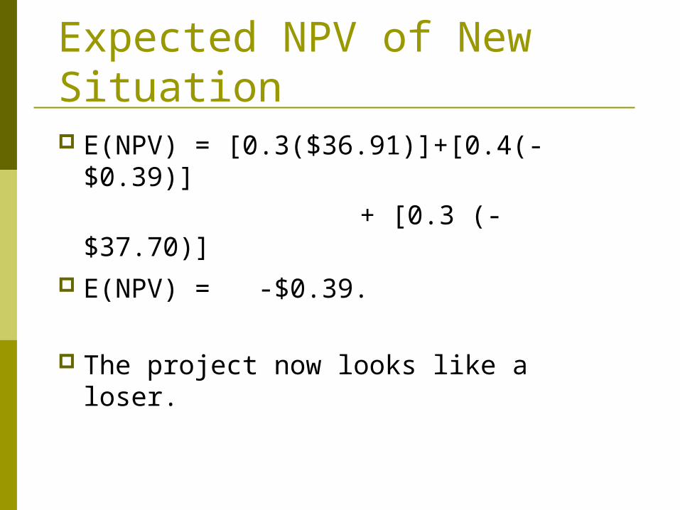
Expected NPV of New Situation E(NPV) = [0.3($36.91)]+[0.4(-$0.39)] + [0.3 (-$37.70)] E(NPV) = -$0.39.
The project now looks like a loser.

Growth Option: You can replicate the original project after it ends in 3 years.
NPV = NPV Original + NPV Replication= -$0.39 + -$0.39/(1+0.10)3 = -$0.39 + -$0.30 = -$0.69.
Still a loser, but you would implement Replication only if demand is high.
Note: the NPV would be even lower if we separately discounted the $75 million cost of Replication at the risk-free rate.

Decision Tree Analysis
Notes: The Year 3 CF includes the cost of the project if it is optimal to replicate. The cost is discounted at the risk-free rate, other cash flows are discounted at the cost of capital.
Cost NPV thisYear 0Prob. 1 2 3 4 5 6 Scenario
$45 $45 -$30 $45 $45 $45 $58.0230%
-$75 40% $30 $30 $30 $0 $0 $0 -$0.3930%
$15 $15 $15 $0 $0 $0 -$37.70
Future Cash Flows

Expected NPV of Decision Tree E(NPV) = [0.3($58.02)]+[0.4(-$0.39)] + [0.3 (-$37.70)] E(NPV) = $5.94.
The growth option has turned a losing project into a winner!

Financial Option Analysis: Inputs X = exercise price = cost of implement
project = $75 million. rRF = risk-free rate = 6%. t = time to maturity = 3 years.

Estimating P: First, find the value of future CFs at exercise year.
Example: $111.91 = $45/1.1 + $45/1.12 + $45/1.13.
Cost PV at Prob.Year 0Prob. 1 2 3 4 5 6 Year 3 x NPV
$45 $45 $45 $33.5730%40% $30 $30 $30 $74.61 $29.8430%
$15 $15 $15 $37.30 $11.19
Future Cash Flows
$111.91

Now find the expected PV at the current date, Year 0.
PVYear 0=PV of Exp. PVYear 3 = [(0.3* $111.91) +(0.4*$74.61)
+(0.3*$37.3)]/1.13 = $56.05.
PVYear 0 Year 1 Year 2 PVYear 3
$111.91High
$56.05 Average $74.61Low
$37.30

The Input for P in the Black-Scholes Model
The input for price is the present value of the project’s expected future cash flows.
Based on the previous slides,P = $56.05.

Estimating 2: Find Returns from the Present until the Option Expires
Example: 25.9% = ($111.91/$56.05)(1/3) - 1.
AnnualPVYear 0 Year 1Year 2 PVYear 3 Return
$111.91 25.9%High
$56.05Average $74.61 10.0%Low
$37.30 -12.7%
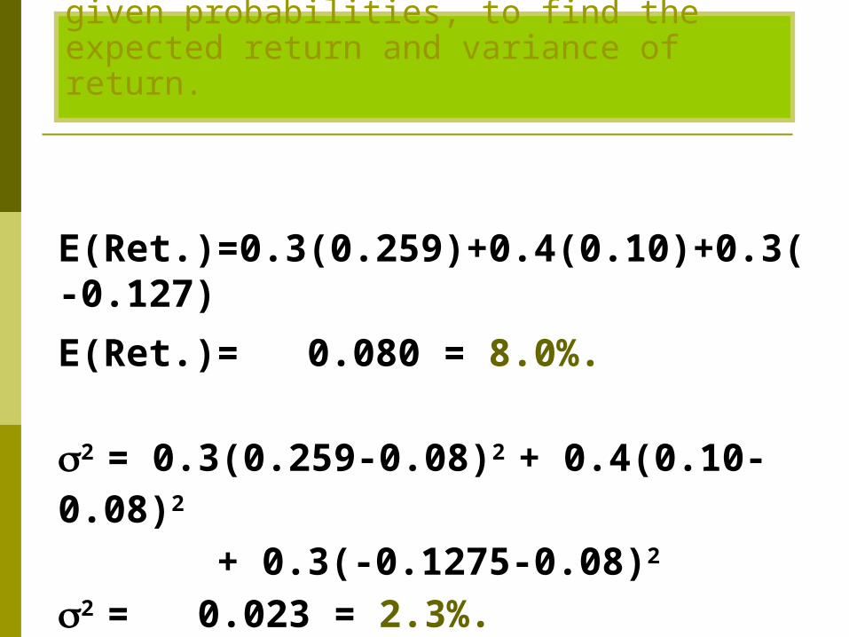
E(Ret.)=0.3(0.259)+0.4(0.10)+0.3(-0.127)
E(Ret.)= 0.080 = 8.0%.
2 = 0.3(0.259-0.08)2 + 0.4(0.10-0.08)2
+ 0.3(-0.1275-0.08)2
2 = 0.023 = 2.3%.
Use these scenarios, with their given probabilities, to find the expected return and variance of return.

Why is 2 so much lower than in the investment timing example?
2 has fallen, because the dispersion of cash flows for replication is the same as for the original project, even though it begins three years later. This means the rate of return for the replication is less volatile.
We will do sensitivity analysis later.

Estimating 2 with the Indirect Method
PVYear 3
$111.91High
Average $74.61Low
$37.30
From earlier slides, we know the value of the project for each scenario at the expiration date.

E(PV)=.3($111.91)+.4($74.61)+.3($37.3)
E(PV)= $74.61.
Use these scenarios, with their given probabilities, to find the project’s expected PV and PV.
PV = [.3($111.91-$74.61)2
+ .4($74.61-$74.61)2 + .3($37.30-$74.61)2]1/2
PV = $28.90.

Now use the indirect formula to estimate 2.
CVPV = $28.90 /$74.61 = 0.39. The option expires in 3 years, t=3.
%7.43
]139.0ln[ 22

Use the Black-Scholes Model: P = $56.06; X = $75; rRF = 6%;
t = 3 years: 2 = 0.047
V = $56.06[N(d1)] - $75e-(0.06)(3)[N(d2)].
ln($56.06/$75)+[(0.06 +0.047/2)](3)
(0.047)0.5 (3).05
= -0.1085.
d2 = d1 - (0.047)0.5 (3).05= d1 - 0.3755
= -0.1085 - 0.3755 =- 0.4840.
d1 =

N(d1) = N(0.2641) = 0.4568N(d2) = N(- 0.1127) = 0.3142
V = $56.06(0.4568) - $75e(-0.06)(3)(0.3142) = $5.92.
Note: Values of N(di) obtained from Excel using
NORMSDIST function.

Total Value of Project with Growth OpportunityTotal value = NPV of Original Project + Value
of growth option
=-$0.39 + $5.92
= $5.5 million.

Sensitivity Analysis on the Impact of Risk (using the Black-Scholes model) If risk, defined by 2, goes up, then value
of growth option goes up: 2 = 4.7%, Option Value = $5.92 2 = 14.2%, Option Value = $12.10 2 = 50%, Option Value = $24.08
Does this help explain the high value many dot.com companies had before 2002?

82
Project Analysis Under Certainty: Recap
Discounted cash flow techniquesThe ideal investment decision makingtechnique is Net Present Value.N P V measures the equivalent presentwealth contributed by the investment. NPV-- relates directly to the firm’s goal of wealth maximization -- employs the time value of money -- can be used in all types of investments
-- can be adjusted to incorporate risk.

83
Other Project Evaluation Techniques
Internal Rate of Return – calculatesThe discount rate that gives theproject an NPV of 0. If the IRR isgreater than the required rate, theproject is accepted. IRRis given as % pa.
IOIRR
CF
IRR
CFNPV
......
)1()1()(0$
22
11

Other Project Evaluation Techniques
Modified Internal Rate of Return – calculates the discount rate that gives the project an NPV of $0, when future cash flows can be re-invested at the Re-Investment Rate, a rate different from the IRR. If the MIRR is greater that the required rate, the project is accepted. MIRR is given as % pa.
IOIRR
RIRCF
IRR
RIRCFNPV
nn
......)1(
)1(
)1(
)1()(0$
2
)1(2
11

85
Other Project Evaluation Techniques
Non-Discounted Cash Flow Techniques
Accounting Rate of Return- measures the ratioof annual average accounting income to anasset base value. ARR is given as % pa. Payback Period – measures the length of timerequired to retrieve the initial cash outlay. Payback is given as number of years.

86
Selection of Techniques
NPV is the technique of choice; it satisfies therequirements of: the firm’s goal, the time value ofmoney, and the absolute measure of investment.
IRR is useful in a single asset case, where theCash flow pattern is an outflow followed by allpositive inflows. In other situations the IRR maynot rank mutually exclusive assets properly, ormay have zero or many solutions.

87
Selection of TechniquesMIRR is useful in the same situations as the IRR, but requires the extra prediction of a re-investment rate.
ARR allows many valuations of the asset base, does not account for the time value of money, and does not relate to the firm’s goal. It is not a recommended method.
PB does not allow for the time value of money, and does not relate to the firm’s goal. It is not a recommended method except for situations of uncertainty.

88
The Notion of Certainty Certainty assumption
Financial decision makers are rational, risk-averse, wealth maximizers
Financial markets are efficient and competitive Future is certain, outcome is known
Certainty allows demonstration and evaluation of the capital budgeting techniques, whilst avoiding the complexities involved with risk.
Certainty requires forecasting, but forecasts which are certain.
Certainty is useful for calculation practice. Risk is added as an adaption of an evaluation
model developed under certainty.

89
NPV Applications•Asset retirement
•Asset replacement
•Correct ranking of mutually exclusive projects.
•Where projects have different lives.
•Where projects have different outlays.
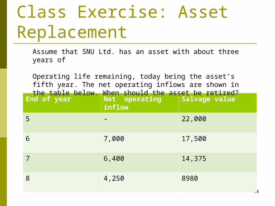
Class Exercise: Asset Replacement
90
End of year Net operating inflow
Salvage value
5 - 22,000
6 7,000 17,500
7 6,400 14,375
8 4,250 8980
Assume that SNU Ltd. has an asset with about three years of
Operating life remaining, today being the asset’s fifth year. The net operating inflows are shown in the table below. When should the asset be retired?

Net Present Value
THE model to use in all investmentevaluations.Other criteria, such as IRR, MIRR, ARR,and Payback may be used as complementary measures.

92
Class Exercise
Consider the following three cash flow profiles:
Year ending
0 1 2 3 4 5
Project 1 -100 20 20 20 20 120
Project 2 -100 33.44 33.44 33.44 33.44 33.44
Project 3 -100 85.22 85.22 85.22 85.22 -300
Calculate IRR, NPV, and Payback periods for the projects

93
Class ExerciseProject IRR(%) NPV Payback
1 20 37.9 5
2 20 26.8 3
3 19.9, 44.4 -16.4 1.2

94
Pitfalls in Project Appraisal Specifying project’s incremental cash flow
requires care Relevant expected after-tax cash flow associated with
two mutually exclusive scenarios, without and with the project
Allocation of overheads Expected versus most likely cash flows
Mean versus mode Limited capacity
The IRR is biased The IRR’s of projects with different cash flow profiles are
not comparable Projects with equal IRR can have different NPVs when
they have different payback periods IRR calculation uses IRR itself as the discount rate

95
Pitfalls in Project Appraisal The payback period is often ambiguous
Does not reflect the time value of money Ignores cash flows after the payback period Unsuitable for projects requiring investment over a period of
years Discount rates are frequently wrong
Fallacy of single discount rate, projects have widely differing risks
Rising inflation rates are dangerous Use of a nominal rate to discount nominal cash flows and use
of a real rate to discount real cash flows All cash flows do not change equally with the rate of inflation Inflation increases the required investment in nominal working
capital Inflation increases corporate tax rate

96
Pitfalls in Project Appraisal The precise timing of cash flows is important
Cash flows occur at the end of the year assumption Two methods for precise discounting
Use monthly discount rates For example 1.5 –year discount factor
Forecasting is often untruthful Increase the hurdle rate by the average forecasting bias Subsidiary forecast
Risk adds value to real options Real options affect the NPV rule

97
Critique of DCF Ignores risks inherent in capital projects
Uses the same discount rate to cash flows with different risks
Uses the same discounts rates throughout the life of the project
Considers investment one-time irreversible decision

98
Real Options in Capital Projects Simply adjusting the discount rate for the risk
does not account for the full impact of uncertainty Uncertainty affects investment in two ways
Uncertainty about investment (I) required Uncertainty about the present value (PV) that the future
investment might generate Since the future values (FVs) of I and PV may
both be uncertain, we need to simplify by combing them into a single variable:Profitability index = Present value/Investment
PI = PV/I

99
Real Options in Capital Projects Real option and profitability index
Exercise real option only if PI turns out to be greater than of equal to 1.00
Otherwise, keep the funds I invested in the financial market where PI virtually always equals 1.00

100
Uncertainty and Real Options Value In the year 2000 GROWTHCO had a prospective project
under development The decision to invest will not be made until 2003 Investment in the project is contingent upon PI being
greater than 1 Therefore, in 2000 the potential to invest in 2003 was a real
option for GROWTHCO Management expected to invest $25 million in the project if
PI>1 R&D budget to make the project ready is $ 1 million per
year. The actual size of the investment is uncertain, it depended
on market information fully available until 2003 Real options payoff histogram

101
Real Options in Capital Projects
0 0.4 0.8
Probability
1.0 1.4 1.8 2.0
Real Option Payoff Histogram
PI

102
Calculation of expected PI of payoffInterval
(1)Interval value
(2)Probability
(3)PI of payoff
(4)Expected PI of payoff
(3x4)
0<x<=0.4 0.2 0.16 1.00 0.160
0.4<x<=0.8 0.6 0.21 1.00 0.210
0.8<x<=1.2 1 0.26 1.05 0.273
1.2<x<=1.6 1.4 0.21 1.40 0.294
1.6<x<=2 1.8 0.16 1.80 0.288
1.00 1.225

103
Calculation of the Expected PI of Payoff
The first column shows selected intervals of the PI used in the histogram
The second column is the average value of the PI for each interval
The third column gives the probability management assigned to each interval
The fourth column gives the value of the PI of the payoff depending on whether or not management would exercise the investment option
The final column gives the product of the PI and its probability for each interval
The sum at the bottom of the column gives the expected PI of the payoff

104
Calculation of the Expected PI of Payoff
For example, in the fourth row PI falls between 1.2 and 1.6 The second column shows the average value of the interval, 1.4 The third column shows the probability management assigned to
this interval, 0.21 Because the average interval value of 1.4 is greater than 1,
management would intend to invest in this interval, gaining an average PI value of 1.4 with probability of 0.21
The final column gives the product of the PI value (1.4) and its probability(0.21)i.e. 0.294
The first two rows PI value is less than 1, management under these circumstances would invest in financial market and get a value of 1.00, as shown in the fourth column
The third row has an interval value of 1. Therefore we use weighted average 0.5x1.1+0.5x1=1.05
The expected value of the investments PI with option payoff is 1.225 as shown at the bottom row

105
Risk Neutral Valuation of Real Options
Management’s option to reject the unfavorable payoffs alters distributions of PI
Risk adjustment factorF = Risk adjustment factor for PV/ Risk adjustment factor for I Risk adjustment factor for PV= (1+RF)T/ (1+RPV)T
Risk adjustment factor for I= (1+RF)T/ (1+RI)T
Therefore, F = (1+RI)T/ (1+RPV)T , where
RI represents the discount rate for future investment expenditure and RPV is the Project’s discount rate
Assuming RI= 0.5 and RPV=0.10, we get F=0.870 Multiply all the class intervals by the risk-adjustment
factor

106
Real Options in Capital Projects
0 0.37 0.75
Probability
1.0
1.12 1.49 1.87
Risk adjusted Histogram
PI

107
Risk-neutral Valuation of the expected PI with payoff
Interval Risk-neutral interval
Interval value
Probability PI of payoff Expected PI of payoff
0<x<=0.4 0<x<=0.37 0.18 0.16 1.00 0.160
0.4<x<=0.8 0.37<x<=0.74 0.55 0.21 1.00 0.210
0.8<x<=1.2 0.74<x<=1.10 0.92 0.26 1.01 0.264
1.2<x<=1.6 1.10<x<=1.47 1.29 0.21 1.29 0.271
1.6<x<=2 1.47<x<=1.84 1.66 0.16 1.66 0.265
1.00 1.169

108
Risk Neutral Valuation of Real Options
Re-calculate other values using the risk-neutral intervals. The result is a smaller expected PI payoff 1.169
Present value of the option= Present value of the expected investment expenditure * (Present value of the PI-1)
= $25/(1+0.07)3*(1.169-1)= $3.449 million R&D budget to make the project ready is $ 1 million per
year. The present value of this three year annuity discounted at 5% is $2.723 million
Therefore, addition to shareholder value, due to exercising this option, is $3.449 - $2.723 million = 0.726 million
R&D should go ahead