Embed Size (px)
Citation preview
Under consideration for publication in Math. Proc. Camb. Phil. Soc. 1
Extreme values of some continuous
nowhere differentiable functions
By PIETER C. ALLAART and KIKO KAWAMURA
University of North Texas †
(Received )
Abstract
We consider the functions Tn(x) defined as the n-th partial derivative of Lebesgue’s
singular function La(x) with respect to a at a = 12 . This sequence includes a multiple
of the Takagi function as the case n = 1. We show that Tn is continuous but nowhere
differentiable for each n, and determine the Holder order of Tn. From this, we derive
that the Hausdorff dimension of the graph of Tn is one. Using a formula of Lomnicki and
Ulam, we obtain an arithmetic expression for Tn(x) using the binary expansion of x, and
use this to find the sets of points where T2 and T3 take on their absolute maximum and
minimum values. We show that these sets are topological Cantor sets. In addition, we
characterize the sets of local maximum and minimum points of T2 and T3.
AMS 2000 subject classification: Primary 26A30,28A80; Secondary 26A27.
† authors’ address: Mathematics Department, P.O. Box 311430, Denton, TX 76203-1430,
USA; e-mail: [email protected], [email protected]
2 Pieter C. Allaart and Kiko Kawamura
Key words and phrases: Takagi function, Lebesgue’s singular function, Hausdorff di-
mension, Extreme values, Nowhere differentiable continuous function, Holder order
1. Introduction
Let La(x) be Lebesgue’s singular function with a real parameter a (0 < a < 1, a �= 12 ).
As is well known, La(x) is strictly increasing and has a derivative equal to zero almost
everywhere. In 1991, Sekiguchi and Shiota [14] proved that La(x) is an analytic function
with respect to a for each fixed x in [0, 1], and studied the functions
Tr,n(x) :=1n!
∂nLa(x)∂an
∣∣∣∣a=r
, n = 1, 2, 3, . . . , 0 < r < 1.
In this paper, we consider the case r = 12 and define
Tn(x) :=1n!
∂nLa(x)∂an
∣∣∣∣a= 1
2
, n = 1, 2, 3, . . . . (1·1)
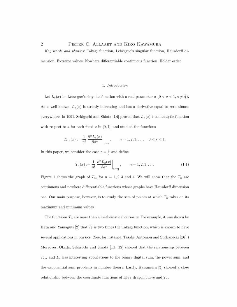
Figure 1 shows the graph of Tn, for n = 1, 2, 3 and 4. We will show that the Tn are
continuous and nowhere differentiable functions whose graphs have Hausdorff dimension
one. Our main purpose, however, is to study the sets of points at which Tn takes on its
maximum and minimum values.
The functions Tn are more than a mathematical curiosity. For example, it was shown by
Hata and Yamaguti [2] that T1 is two times the Takagi function, which is known to have
several applications in physics. (See, for instance, Tasaki, Antoniou and Suchanecki [16].)
Moreover, Okada, Sekiguchi and Shiota [11, 12] showed that the relationship between
Tr,n and La has interesting applications to the binary digital sum, the power sum, and
the exponential sum problems in number theory. Lastly, Kawamura [5] showed a close
relationship between the coordinate functions of Levy dragon curve and Tn.
Extreme values of cnd functions 3
1.2
0.8
0.0
1.0
0.6
0.2
0.4
0.80 10.2 0.4 0.6
1.5
0.5
-1.5
1.0
0.0
-1.0
-0.5
0.8 10.2 0.4 0.6
3
1
2
0
-1
0.6 0.8 10.2 0.4
4
0
2
-2
-4
0.6 0.8 10.2 0.4
Fig. 1. Graphs of T1 (top left), T2 (top right), T3 (bottom left) and T4 (bottom right).
The Takagi function, introduced first by Takagi in 1903 [15], is one of the simplest
examples of a continuous, nowhere differentiable function. It is given by
T (x) =∞∑
k=0
12kψ(2kx), 0 ≤ x ≤ 1, (1·2)
where ψ(x) = |x − �x + 12�|. The Takagi function was rediscovered independently by
other mathematicians, e.g. Knopp in 1918, Hobson in 1926, Van der Waerden in 1930,
Hildebrandt in 1933, and De Rham in 1957. It is known alternatively as the Van der
Waerden function, or the Takagi-Van der Waerden function.
Several authors have studied properties of the Takagi function. For example, in 1959,
Kahane [4] showed that the set of points at which the Takagi function attains its
maximum value is a Cantor set, and the maximum value is 23 . In 1986, Mauldin and
Williams [10] introduced a new geometric property of a function: convex Lipschitz of
order θ, and used this to show, among other things, that the graph of the Takagi func-
4 Pieter C. Allaart and Kiko Kawamura
tion has Hausdorff dimension one. Kairies [3] gave several functional equations which
the Takagi function satisfies, and discussed their relationship. A more general class of
functions, called the Takagi class, was introduced by Hata and Yamaguti [2]. A function
f belongs to the Takagi class if it satisfies a system of infinitely many difference equations
of the form
f
(2j + 12k+1
)− 1
2
{f
(j
2k
)+ f
(j + 12k
)}= Ck, (1·3)
for 0 ≤ j ≤ 2k − 1, k = 0, 1, 2, · · · , with the boundary conditions f(0) = f(1) =
0. Here, {Ck} is any given numerical sequence. When Ck = 2−(k+1), f is the Takagi
function. Hata and Yamaguti proved that (1·3) has a unique continuous solution if and
only if∑∞
k=0 |Ck| < ∞. Kono [8] investigated the regularity and the differentiability of
functions of the Takagi class, concluding that f has no finite derivative at any point if
lim supk→∞ 2k|Ck| > 0.
The organization of this article is as follows. Section 2 gives the functional equations
and a system of infinitely many difference equations having Tn as a solution. These
equations show that the Tn are not self-affine in the sense of Kono [7], and do not belong
to the Takagi class when n ≥ 2. Section 3 gives an arithmetic expression for Tn(x) using
the binary expansion of x. This representation is the key to many of the later results of
the paper. In section 4, we show that
Tn(x+ y) − Tn(x) = O(|y|(log(1/|y|))n) as y → 0,
from which it follows that the Hausdorff dimension of the graph of Tn is one. In section 5,
we prove that the Tn are nowhere differentiable.
Section 6 treats the problem of finding maximum and minimum points of Tn. It begins
by reviewing Kahane’s result on the maximum points of the Takagi function, which is
Extreme values of cnd functions 5
one half times T1. Not surprisingly, the problem becomes more difficult as n increases.
However, using the arithmetic expression from section 3, we can - at least in principle -
find the extremal points of Tn by studying the roots and local extrema of a particular
sequence of functions, made up of an exponential factor and a polynomial factor of degree
n. Unfortunately, this analysis is feasible only for n = 2 or 3, as no simple expressions
are available for the roots of the polynomial when n ≥ 4. We find that both the sets of
maximum points and the sets of minimum points of T2 and T3 are topological Cantor
sets, and are therefore uncountably large. (By contrast, we conjecture that the sets of
maximum and minimum points of Tn are finite when n ≥ 4.) Specifically, the maximum
points of T2 are exactly those points of the form
x = .00
01
or
10
010
01
or
10
01010
01
or
10
0101010
01
or
10
010101010
01
or
10
· · · ,
while the minimum points are obtained by interchanging zeros and ones in the above
pattern. Similarly, the maximum points of T3 lying in the interval [0, 12 ] are exactly those
6 Pieter C. Allaart and Kiko Kawamura
points of the form
x = .0000
01
or
10
0
01
or
10
010︸︷︷︸ 010︸︷︷︸
01
or
10
010︸︷︷︸
01
or
10
01010︸ ︷︷ ︸ 01010︸ ︷︷ ︸
01
or
10
01010︸ ︷︷ ︸
01
or
10
0101010︸ ︷︷ ︸ 0101010︸ ︷︷ ︸
01
or
10
0101010︸ ︷︷ ︸
01
or
10
010101010︸ ︷︷ ︸ 010101010︸ ︷︷ ︸
01
or
10
· · · .
Interestingly, the set of minimum points of T3 is found to coincide with the set of maxi-
mum points of T1. The graphs in Figure 1 illustrate this coincidence.
In subsection 6·4, we introduce a general procedure for constructing a point x with
a “large” value of Tn(x). This algorithm, which places every next “1” in the binary
expansion of x so as to achieve the greatest immediate increase in the value of Tn(x), will
be called the max-greedy algorithm. A dual version, the min-greedy algorithm, produces
a “small” value of Tn(x). We show that these greedy algorithms actually attain the
maximum and minimum values of T2 and T3. Numerical evidence suggests that the
greedy algorithms continue to be optimal for larger values of n, but we have not been
able to prove this.
In subsection 6·5, we consider the local extrema of Tn(x). We show how a dense set of
local extreme points can be obtained from any global extreme point, and give complete
characterizations of the local maximum and minimum points of T2 and T3. The paper
ends with a discussion of some unsolved problems and conjectures.
Extreme values of cnd functions 7
2. Functional equations
First, we derive functional equations for the Tn. In 1983, Yamaguti and Hata [18]
proved the following general theorem.
Theorem 2·1 (Yamaguti-Hata, 1983). Let (t, x) ∈ (−1, 1) × [0, 1], ψ : [0, 1] → [0, 1]
and g : [0, 1] → R. The functional equation F (t, x) = tF (t, ψ(x)) + g(x) has a unique
bounded solution F (t, x), which is given by F (t, x) =∑∞
n=0 tng(ψn(x)).
As an example of this theorem, Yamaguti and Hata showed that T1(x) is the unique
bounded solution of the following functional equation:
T1(x) =
12T1(2x) + 2x, 0 ≤ x ≤ 1
2 ,
12T1(2x− 1) + 2(1 − x), 1
2 ≤ x ≤ 1.
(2·1)
It was shown by De Rham [13] that La(x) is the unique continuous solution of the
functional equation
La(x) =
aLa(2x), 0 ≤ x ≤ 1
2 ,
(1 − a)La(2x− 1) + a, 12 ≤ x ≤ 1.
(2·2)
Differentiating this n times with respect to a gives
∂nLa(x)∂an
=
a∂nLa(2x)∂an + n∂n−1La(2x)
∂an−1 , 0 ≤ x < 12 ,
(1 − a)∂nLa(2x−1)∂an − n∂n−1La(2x−1)
∂an−1 , 12 ≤ x ≤ 1,
for n = 2, 3, · · · . Thus, by Definition 1·1 we have the following result.
Proposition 2·2. For each n ≥ 2, Tn(x) is the unique bounded solution, given the
8 Pieter C. Allaart and Kiko Kawamura
function Tn−1, of the following functional equation.
Tn(x) =
12Tn(2x) + Tn−1(2x), 0 ≤ x ≤ 1
2 ,
12Tn(2x− 1) − Tn−1(2x− 1), 1
2 ≤ x ≤ 1.
(2·3)
From the above equation, we can see that the graphs of the Tn have the following
symmetry properties.
Corollary 2·3. For each n ∈ N and x ∈ [0, 1], Tn(x) = (−1)n−1Tn(1 − x).
Corollary 2·4. For each n ≥ 2, Tn(x) satisfies the following functional equations.
Tn
(x2
)+ Tn
(x+ 1
2
)= Tn(x), 0 ≤ x ≤ 1, (2·4)
Tn
(x2
)− Tn
(x+ 1
2
)= 2Tn−1(x), 0 ≤ x ≤ 1. (2·5)
Conversely, (2·4) and (2·5) uniquely determine Tn, given Tn−1.
The functional equation (2·1) yields the following system of infinitely many difference
equations having T1(x) as a unique bounded solution:
T1
(2j + 12k+1
)− 1
2
{T1
(j
2k
)+ T1
(j + 12k
)}= 2−k, (2·6)
for 0 ≤ j ≤ 2k − 1, k = 0, 1, 2, · · · , with the boundary conditions T1(0) = T1(1) = 0. By
the remark following (1·3), this implies that T1 is twice the Takagi function.
Similarly, from the functional equation (2·3), we have
Corollary 2·5. If n ≥ 2, then Tn(x) satisfies the following system of infinitely many
difference equations.
Tn
(2j + 12k+1
)− 1
2
{Tn
(j
2k
)+ Tn
(j + 12k
)}= Tn−1
(j + 12k
)− Tn−1
(j
2k
), (2·7)
for 0 ≤ j ≤ 2k − 1, k = 0, 1, 2, · · · , with the boundary conditions Tn(0) = Tn(1) = 0.
Extreme values of cnd functions 9
Proof. From (2·1) and (2·3), we derive that Tn(0) = Tn(1) = 0 for all n ∈ N. From
(2·3), it follows that
Tn(12 ) − 1
2{Tn(0) + Tn(1)} = 12Tn(1) + Tn−1(1) = 0 = Tn−1(1) − Tn−1(0).
It is now straightforward to show (2·7) by induction on k. (The induction step involves
using (2·3) in the forward direction for each term in the left side of (2·7), applying the
induction hypothesis to those terms having a numerator 2j + 1, rearranging terms, and
finally using (2·3) in the reverse direction with n− 1 in place of n.)
A different proof of equation (2·7) was given by Sekiguchi and Shiota [14]. Note that
the right hand side of (2·7) depends on j as well as on k. Therefore, Tn does not belong
to the Takagi class when n ≥ 2.
Finally, we note that the functions Tn, n ∈ N are not self-affine in the sense of Kono.
Recall that a function f : [0, 1] → R is called self-affine in the sense of Kono if there exist
a ∈ N and b > 0 such that f((x + i)/a) − f(i/a) = f(x)/b or −f(x)/b for all 0 ≤ x < 1
and i = 0, 1, · · · , a−1. Kono [7] studied the differentiability and the Holder order of self-
affine functions. In 1990, Urbanski [17] showed how to calculate the Hausdorff dimension
of the graph of any continuous self-affine function.
3. An arithmetic expression for Tn(x)
Below we derive an expression for Tn(x) that lies on the basis of many of the later
results of this paper.
Let the binary expansion of x ∈ [0, 1] be denoted by
x =∞∑
k=1
ωk2−k, ωk = ωk(x) ∈ {0, 1}.
For those x ∈ [0, 1] having two binary expansions, we choose the expansion which is
10 Pieter C. Allaart and Kiko Kawamura
eventually all zeroes. As an exception, fix ωk = 1 for every k if x = 1. Let qk = qk(x) =
∑kj=1 ωj ; in other words, qk is the number of 1’s occurring in the first k binary digits of
x. By convention, q0 = 0.
The arithmetic expression follows by diffentiating the following formula of Lomnicki
and Ulam [9]:
La(x) =a
1 − a
∞∑k=1
ωkak−qk(1 − a)qk , 0 ≤ x ≤ 1, (3·1)
where 0 < a < 1.
Theorem 3·1. For each n ∈ N, Tn(x) has the following representation:
Tn(x) =∞∑
k=1
ωk
(12
)k−n n∑i=0
(−1)i
(qk − 1i
)(k − qk + 1n− i
), 0 ≤ x ≤ 1.
Proof. If f(a) = (1 − a)m and g(a) = al, Leibniz’s rule implies
dn
dan{f(a)g(a)} =
n∑i=0
(n
i
)f (i)(a)g(n−i)(a)
=n∑
i=0
(n
i
)(m
i
)(l
n− i
)i!(n− i)!(1 − a)m−ial−n+i(−1)i
= n!n∑
i=0
(m
i
)(l
n− i
)(1 − a)m−ial−n+i(−1)i.
Using this with m = qk − 1 and l = k − qk + 1 gives, from (1·1) and (3·1):
Tn(x) =1n!
∞∑k=1
ωk∂n
∂an
{(1 − a)qk−1ak−qk+1
}∣∣∣∣a= 1
2
=∞∑
k=1
ωk
(12
)k−n n∑i=0
(−1)i
(qk − 1i
)(k − qk + 1n− i
).
Theorem 3·1 shows that, for example,
T1(x) =∂La(x)∂a
∣∣∣∣a= 1
2
=∞∑
k=1
ωk
(12
)k−1
{k + 2 − 2qk} ,
a formula that has already appeared in [5].
Extreme values of cnd functions 11
Definition 3·2. For each n ∈ N, define the function
fn(t, q) :=(
12
)t−n n∑i=0
(−1)i
(q − 1i
)(t− q + 1n− i
), t ∈ R, q ∈ N,
where as usual,
(t
i
):=
t(t− 1)(t− 2) · · · (t− i+ 1)i!
, t ∈ R, i ∈ N ∪ {0}.
Lemma 3·3. Let f and f ′ be arbitrary functions from {(k, q) ∈ N × N : k ≥ q} to
R, and let S(x) =∑∞
k=1 ωk(x)f(k, qk(x)), and S′(x) =∑∞
k=1 ωk(x)f ′(k, qk(x)). Then
S(x) = S′(x) for all x if and only if f(k, q) = f ′(k, q) for all k ∈ N and 1 ≤ q ≤ k.
Proof. Let W (x) = S(x)−S′(x) and h(k, q) = f(k, q)−f ′(k, q). Suppose W (x) = 0 for
all x. Especially, 0 = W (2−k) = h(k, 1) for all k. Similarly, 0 = W (2−1 +2−k) = h(1, 1)+
h(k, 2) = h(k, 2) for all k ≥ 2, etc. Continuing this argument yields that h(k, q) = 0 for
q ∈ N and k ≥ q. The lemma follows.
Corollary 3·4. For all k, q ∈ N and n ≥ 2,
fn(k, q) − fn(k + 1, q) = fn(k + 1, q + 1), (3·2)
Proof. Since (2·4) shows that
∞∑k=1
ωkfn(k + 1, qk) +
{ ∞∑k=1
ωkfn(k + 1, qk + 1) + fn(1, 1)
}=
∞∑k=1
ωkfn(k, qk),
and fn(1, 1) = 0 if n ≥ 2, (3·2) follows from Lemma 3·3.
Of course, Corollary 3·4 can also be proved using identities for binomial coefficients.
4. Holder order and Hausdorff dimension of Tn
In this section, we establish the Holder order of Tn, and show that the graph of Tn has
Hausdorff dimension one.
12 Pieter C. Allaart and Kiko Kawamura
Theorem 4·1. For each n ∈ N, there exist positive constants Cn and δn such that if
0 ≤ x < x+ y ≤ 1 and y < δn, then
|Tn(x+ y) − Tn(x)| ≤ Cny(log2(1/y))n.
Moreover, the function y(log2(1/y))n can not be replaced by a function of smaller order.
Proof. We will show that if 0 ≤ x < x+ y ≤ 1 and y < 2−n, then
|Tn(x+ y) − Tn(x)| ≤ 22n+3
n!y(log2(1/y))
n.
Note first that for all k and q,
|fn(k, q)| ≤ 2−(k−n)n∑
i=0
(q − 1i
)(k − q + 1n− i
)= 2−(k−n)
(k
n
).
Thus, if ξ ∈ [0, 1], j/2N ≤ ξ < (j + 1)/2N and N ≥ n, then by Theorem 3·1,
|Tn(ξ)−Tn(j/2N)| =
∣∣∣∣∣∞∑
k=N+1
ωk(ξ)fn(k, qk(ξ))
∣∣∣∣∣≤
∞∑k=N+1
|fn(k, qk(ξ))| ≤∞∑
k=N
2−(k−n)
(k
n
)
= 2−(N−n)
(N
n
) ∞∑k=N
2−(k−N) k(k − 1) · · · (k − n+ 1)N(N − 1) · · · (N − n+ 1)
= 2−(N−n)
(N
n
) ∞∑l=0
2−l
(1 +
l
N
)(1 +
l
N − 1
)· · ·(
1 +l
N − n+ 1
)
≤ 2−(N−n)
(N
n
) ∞∑l=0
2−l
(1 +
l
n
)(1 +
l
n− 1
)· · · (1 + l)
= 2−(N−n)
(N
n
) ∞∑l=0
2−l
(n+ l
n
)= 2−(N−n)
(N
n
)2n+1
≤ 22n+2
n!Nn2−(N+1).
(4·1)
Now fix x and y satisfying 0 ≤ x < x + y ≤ 1 and y < 2−n, and let N be the integer
such that 2−(N+1) ≤ y < 2−N . Note that N ≥ n. There are two cases to consider.
Case 1. There exists an integer j such that
j
2N≤ x < x+ y <
j + 12N
.
Extreme values of cnd functions 13
Then the first N digits of x, x+ y and j/2N are the same, so by (4·1),
|Tn(x + y) − Tn(x)| ≤ |Tn(x) − Tn(j/2N)| + |Tn(x + y) − Tn(j/2N)|
≤ 2 · 22n+2
n!Nn2−(N+1)
≤ 22n+3
n!y(log2(1/y))
n.
Case 2. There exists an integer j such that
j − 12N
≤ x <j
2N≤ x+ y <
j + 12N
.
In this case, use Corollary 2·3 and (4·1) to obtain
|Tn(x + y) − Tn(x)| ≤ |Tn(x + y) − Tn(j/2N)| + |Tn(j/2N) − Tn(x)|
= |Tn(x + y) − Tn(j/2N)| + |Tn(1 − x) − Tn(1 − j/2N)|
≤ 22n+3
n!y(log2(1/y))
n.
Finally, to see that the bound is best possible, take x = 0 and y = 2−N , and observe
that
Tn(2−N) = fn(N, 1) = 2−(N−n)
(N
n
).
Hence, there exists a constant An such that, for all sufficiently large N ,
Tn(2−N ) ≥ An2−NNn = Any(log2(1/y))n.
This completes the proof.
A consequence of Theorem 4·1 is, that for every ε > 0 there exists a constant Cn,ε such
that if 0 ≤ x < x + y ≤ 1, then |Tn(x + y) − Tn(x)| ≤ Cn,εy1−ε. A standard argument
(e.g. Falconer [1, Theorem 8.1]) thus implies the following:
Corollary 4·2. For each n ∈ N, the graph of Tn has Hausdorff dimension one.
14 Pieter C. Allaart and Kiko Kawamura
5. Nowhere-differentiability of Tn
Since T1 is two times the Takagi function, it is nowhere differentiable. In this section,
we show that the same is true for Tn when n ≥ 2.
Theorem 5·1. For each n ∈ N, Tn is continuous but nowhere differentiable.
Proof. The continuity of Tn follows from Theorem 4·1. To establish the nowhere-
differentiability, let x0 be any point in [0, 1], and consider two cases.
Case 1. If x0 is not a dyadic rational, then there exist integers j1, j2, . . . such that
jk2k
< x0 <jk + 1
2k, k ∈ N.
Define
Pn(k, j) :=Tn
((j + 1) · 2−k
)− Tn
(j · 2−k
)2−k
, k ∈ N, j = 0, 1, . . . , 2k − 1.
We will show by induction on n that limk→∞ Pn(k, jk) does not exist as a real num-
ber. For n = 1, this was proved by Takagi in 1903. So let n ∈ N, and suppose that
limk→∞ Pn(k, jk) does not exist. From (2·7), we derive that
{Pn+1(k + 1, 2jk) − Pn+1(k + 1, 2jk + 1)} = 4Pn(k, jk), (5·1)
for k ∈ N. Let A be the set of those indices k such that jk+1 = 2jk, and note that N\A
consists of those indices k such that jk+1 = 2jk + 1. Since x0 is not a dyadic rational,
both A and N\A are infinite.
Aiming for a contradiction, suppose there exists a finite number m such that
limk→∞
Pn+1(k, jk) = m. (5·2)
Extreme values of cnd functions 15
Reindexing the sequence {(k, jk)} and separating it into two subsequences gives
limk→∞, k∈A
Pn+1(k + 1, 2jk) = m, (5·3)
limk→∞, k �∈A
Pn+1(k + 1, 2jk + 1) = m. (5·4)
Since
Pn+1(k + 1, 2jk) + Pn+1(k + 1, 2jk + 1) = 2Pn+1(k, jk),
(5·2), (5·3) and (5·4) imply that, in fact,
limk→∞
Pn+1(k + 1, 2jk) = limk→∞
Pn+1(k + 1, 2jk + 1) = m.
But by (5·1), this means that limk→∞ Pn(k, jk) = 0, contradicting the induction hypoth-
esis.
Case 2. Assume next that x0 is a dyadic rational, say x0 = j/2N . Since for k > N ,
Tn(x0 + 2−k) − Tn(x0) = fn(k, qN (x0) + 1),
and, for fixed q, fn(k, q) equals 2n−k times a polynomial in k with a positive leading
coefficient, we have
limk→∞
Tn(x0 + 2−k) − Tn(x0)2−k
= +∞. (5·5)
Similarly, using (5·5) with 1 − x0 in place of x0 gives, by Corollary 2·3,
limk→∞
Tn(x0 − 2−k) − Tn(x0)−2−k
= limk→∞
(−1)n−1{Tn(1 − x0 + 2−k) − Tn(1 − x0)
}−2−k
= (−1)n · ∞.
Therefore, we conclude that Tn does not have a finite derivative anywhere.
16 Pieter C. Allaart and Kiko Kawamura
6. Maximum and minimum values of Tn
We call a point x ∈ [0, 1] a maximum point (resp. minimum point) of Tn if Tn takes on
its maximum (resp. minimum) value at x. We denote the set of maximum points of Tn
by S+n , and the set of minimum points by S−
n . The set S+1 was described by Kahane in
1959:
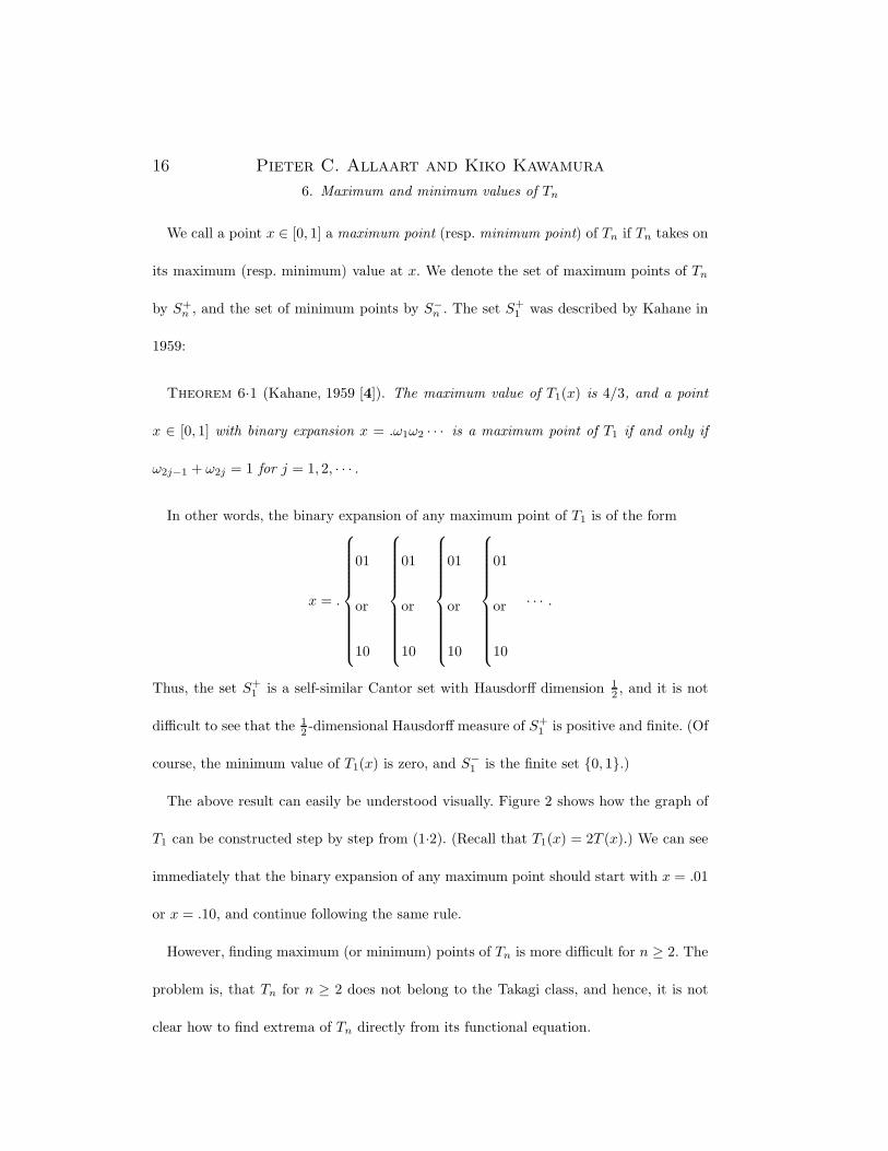
Theorem 6·1 (Kahane, 1959 [4]). The maximum value of T1(x) is 4/3, and a point
x ∈ [0, 1] with binary expansion x = .ω1ω2 · · · is a maximum point of T1 if and only if
ω2j−1 + ω2j = 1 for j = 1, 2, · · · .
In other words, the binary expansion of any maximum point of T1 is of the form
x = .
01
or
10
01
or
10
01
or
10
01
or
10
· · · .
Thus, the set S+1 is a self-similar Cantor set with Hausdorff dimension 1
2 , and it is not
difficult to see that the 12 -dimensional Hausdorff measure of S+
1 is positive and finite. (Of
course, the minimum value of T1(x) is zero, and S−1 is the finite set {0, 1}.)
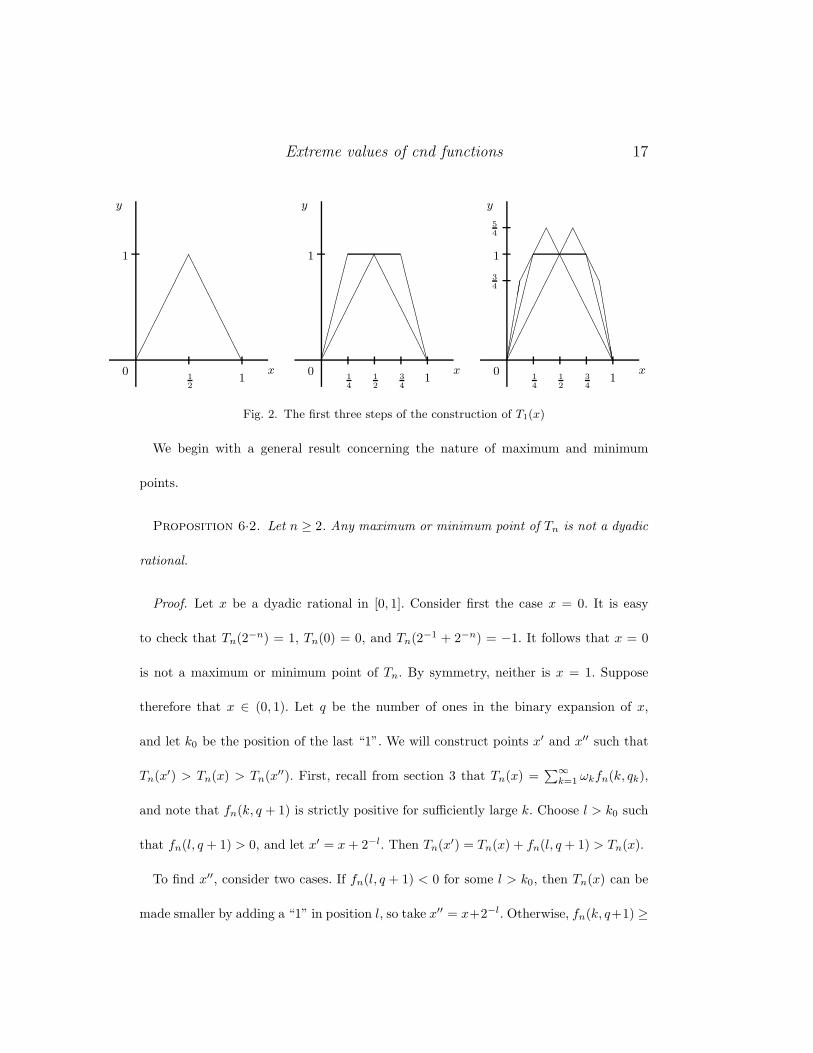
The above result can easily be understood visually. Figure 2 shows how the graph of
T1 can be constructed step by step from (1·2). (Recall that T1(x) = 2T (x).) We can see
immediately that the binary expansion of any maximum point should start with x = .01
or x = .10, and continue following the same rule.
However, finding maximum (or minimum) points of Tn is more difficult for n ≥ 2. The
problem is, that Tn for n ≥ 2 does not belong to the Takagi class, and hence, it is not
clear how to find extrema of Tn directly from its functional equation.
Extreme values of cnd functions 17
���������
�������
x
y
012
1
1
���������
�������
x
y
012
14
34
1
1
�������� �
������� �
��������
�������
x
y
012
14
34
1
54
1
34
�������� �
��������
�����������
����
����������
Fig. 2. The first three steps of the construction of T1(x)
We begin with a general result concerning the nature of maximum and minimum
points.
Proposition 6·2. Let n ≥ 2. Any maximum or minimum point of Tn is not a dyadic
rational.
Proof. Let x be a dyadic rational in [0, 1]. Consider first the case x = 0. It is easy
to check that Tn(2−n) = 1, Tn(0) = 0, and Tn(2−1 + 2−n) = −1. It follows that x = 0
is not a maximum or minimum point of Tn. By symmetry, neither is x = 1. Suppose
therefore that x ∈ (0, 1). Let q be the number of ones in the binary expansion of x,
and let k0 be the position of the last “1”. We will construct points x′ and x′′ such that
Tn(x′) > Tn(x) > Tn(x′′). First, recall from section 3 that Tn(x) =∑∞
k=1 ωkfn(k, qk),
and note that fn(k, q + 1) is strictly positive for sufficiently large k. Choose l > k0 such
that fn(l, q + 1) > 0, and let x′ = x+ 2−l. Then Tn(x′) = Tn(x) + fn(l, q + 1) > Tn(x).
To find x′′, consider two cases. If fn(l, q + 1) < 0 for some l > k0, then Tn(x) can be
made smaller by adding a “1” in position l, so take x′′ = x+2−l. Otherwise, fn(k, q+1) ≥
18 Pieter C. Allaart and Kiko Kawamura
0 for all k > k0, and therefore, by (3·2),
fn(k + 1, q) = fn(k, q) − fn(k + 1, q + 1) ≤ fn(k, q)
for all k ≥ k0. Since fn(k, q) is eventually positive, it follows that fn(k0, q) > 0. This
means Tn(x) will be made smaller by removing the “1” in position k0, so take x′′ =
x− 2−k0 . In both cases, Tn(x′′) < Tn(x).
Proposition 6·2 says that we need only consider points x ∈ [0, 1] having a non-
terminating binary expansion. Observe that for each such x, there is a unique, strictly
increasing sequence {kq}q∈N, such that x =∑∞
q=1 2−kq . Thus, we can write
Tn(x) =∞∑
q=1
fn(kq, q). (6·1)
Which sequence(s) {kq} will maximize the above sum? Which will minimize it? To answer
these questions, an analysis of the functions fn(·, q), for all q ∈ N, is necessary. This
analysis turns out to be feasible only for the cases n = 2 and n = 3.
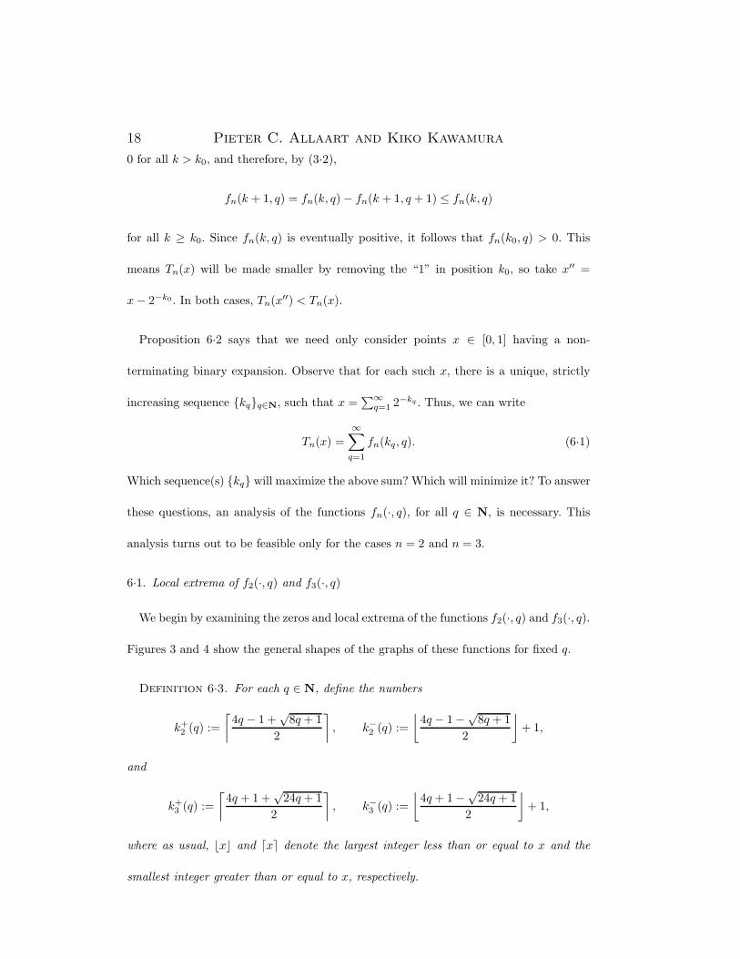
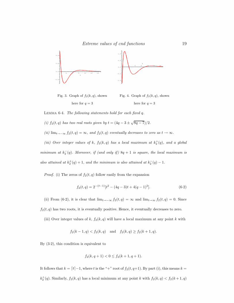
6·1. Local extrema of f2(·, q) and f3(·, q)
We begin by examining the zeros and local extrema of the functions f2(·, q) and f3(·, q).
Figures 3 and 4 show the general shapes of the graphs of these functions for fixed q.
Definition 6·3. For each q ∈ N, define the numbers
k+2 (q) :=
⌈4q − 1 +
√8q + 1
2
⌉, k−2 (q) :=
⌊4q − 1 −√
8q + 12
⌋+ 1,
and
k+3 (q) :=
⌈4q + 1 +
√24q + 1
2
⌉, k−3 (q) :=
⌊4q + 1 −√
24q + 12
⌋+ 1,
where as usual, �x� and �x� denote the largest integer less than or equal to x and the
smallest integer greater than or equal to x, respectively.
Extreme values of cnd functions 19
0.8
0.0
0.4
-0.4
k
141210864
Fig. 3. Graph of f2(k, q), shown
here for q = 3
1.0
0.0
k
0.5
14
-0.5
10642 12
-1.0
8
Fig. 4. Graph of f3(k, q), shown
here for q = 3
Lemma 6·4. The following statements hold for each fixed q.
(i) f2(t, q) has two real roots given by t = (4q − 3 ±√8q − 7)/2.
(ii) limt→−∞ f2(t, q) = ∞, and f2(t, q) eventually decreases to zero as t→ ∞.
(iii) Over integer values of k, f2(k, q) has a local maximum at k+2 (q), and a global
minimum at k−2 (q). Moreover, if (and only if) 8q + 1 is square, the local maximum is
also attained at k+2 (q) + 1, and the minimum is also attained at k−2 (q) − 1.
Proof. (i) The zeros of f2(t, q) follow easily from the expansion
f2(t, q) = 2−(t−1)[t2 − (4q − 3)t+ 4(q − 1)2]. (6·2)
(ii) From (6·2), it is clear that limt→−∞ f2(t, q) = ∞ and limt→∞ f2(t, q) = 0. Since
f2(t, q) has two roots, it is eventually positive. Hence, it eventually decreases to zero.
(iii) Over integer values of k, f2(k, q) will have a local maximum at any point k with
f2(k − 1, q) < f2(k, q) and f2(k, q) ≥ f2(k + 1, q).
By (3·2), this condition is equivalent to
f2(k, q + 1) < 0 ≤ f2(k + 1, q + 1).
It follows that k = �t�−1, where t is the “+” root of f2(t, q+1). By part (i), this means k =
k+2 (q). Similarly, f2(k, q) has a local minimum at any point k with f2(k, q) < f2(k+1, q)
20 Pieter C. Allaart and Kiko Kawamura
and f2(k − 1, q) ≥ f2(k, q), or in other words, with f2(k + 1, q + 1) < 0 ≤ f2(k, q + 1).
Thus k is the integer part of the “− ” root of f2(t, q+1), which by part (i) equals k−2 (q).
Finally, if 8q+1 is square, then f2(t, q+1) has integer roots and, hence, f2(k, q+1) =
f2(k + 1, q + 1) both for k = k+2 (q) and k = k−2 (q) − 1.
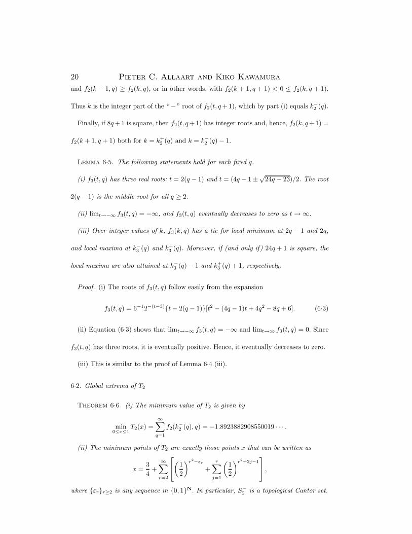
Lemma 6·5. The following statements hold for each fixed q.
(i) f3(t, q) has three real roots: t = 2(q − 1) and t = (4q − 1 ±√24q − 23)/2. The root
2(q − 1) is the middle root for all q ≥ 2.
(ii) limt→−∞ f3(t, q) = −∞, and f3(t, q) eventually decreases to zero as t→ ∞.
(iii) Over integer values of k, f3(k, q) has a tie for local minimum at 2q − 1 and 2q,
and local maxima at k−3 (q) and k+3 (q). Moreover, if (and only if) 24q + 1 is square, the
local maxima are also attained at k−3 (q) − 1 and k+3 (q) + 1, respectively.
Proof. (i) The roots of f3(t, q) follow easily from the expansion
f3(t, q) = 6−12−(t−3){t− 2(q − 1)}[t2 − (4q − 1)t+ 4q2 − 8q + 6]. (6·3)
(ii) Equation (6·3) shows that limt→−∞ f3(t, q) = −∞ and limt→∞ f3(t, q) = 0. Since
f3(t, q) has three roots, it is eventually positive. Hence, it eventually decreases to zero.
(iii) This is similar to the proof of Lemma 6·4 (iii).
6·2. Global extrema of T2
Theorem 6·6. (i) The minimum value of T2 is given by
min0≤x≤1
T2(x) =∞∑
q=1
f2(k−2 (q), q) = −1.8923882908550019 · · · .
(ii) The minimum points of T2 are exactly those points x that can be written as
x =34
+∞∑
r=2
(1
2
)r2−εr
+r∑
j=1
(12
)r2+2j−1 ,
where {εr}r≥2 is any sequence in {0, 1}N. In particular, S−2 is a topological Cantor set.
Extreme values of cnd functions 21
Proof. Recall from Lemma 6·4 that the function k → f2(k, q) has an absolute minimum
value at k−2 (q). Since k−2 (q) is strictly increasing in q, the point x =∑∞
q=1 2−k−2 (q)
minimizes T2(x) in view of (6·1). Part (i) of the theorem follows.
To see part (ii), note that the sequence {k−2 (q)} satisfies
k−2 (q + 1) − k−2 (q) =
1, if 8q + 1 is a square,
2, otherwise.
(6·4)
Furthermore, by Lemma 6·4, f2(k−2 (q), q) = f2(k−2 (q) − 1, q) if and only if 8q + 1 is
a square. This happens exactly when q = r(r + 1)/2 for some r ∈ N, in which case
k−2 (q) = r2, and we can choose either kq = r2 or kq = r2 − 1. The exception is the case
q = 1, where r = 1 and we must choose k1 = 1.
Since T2(x) = −T2(1 − x) for all x, we immediately obtain
Corollary 6·7. (i) The maximum value of T2 is given by
max0≤x≤1
T2(x) = 1.8923882908550019 · · · .
(ii) The maximum points of T2 are exactly those points x that can be written as
x =∞∑
r=2
(1
2
)r2−εr
+r−1∑j=1
(12
)r2+2j ,
where {εr}r≥2 is any sequence in {0, 1}N. In particular, S+2 is a topological Cantor set.
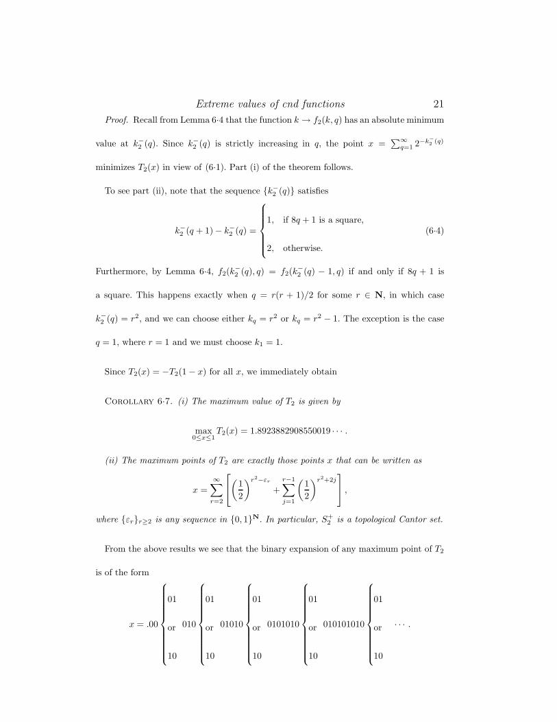
From the above results we see that the binary expansion of any maximum point of T2
is of the form
x = .00
01
or
10
010
01
or
10
01010
01
or
10
0101010
01
or
10
010101010
01
or
10
· · · .
22 Pieter C. Allaart and Kiko Kawamura
1.5
0.5
-1.5
1.0
0.0
-1.0
-0.5
0.8 10.2 0.4 0.6
1.892
1.884
1.888
1.880
0.08 0.0840.081
1.876
0.082 0.083
1.8924
1.8916
1.8920
1.8912
1.8908
0.08090.080750.0806
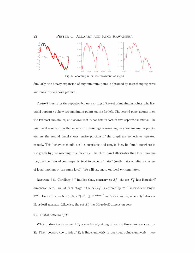
Fig. 5. Zooming in on the maximum of T2(x)
Similarly, the binary expansion of any minimum point is obtained by interchanging zeros
and ones in the above pattern.
Figure 5 illustrates the repeated binary splitting of the set of maximum points. The first
panel appears to show two maximum points on the far left. The second panel zooms in on
the leftmost maximum, and shows that it consists in fact of two separate maxima. The
last panel zooms in on the leftmost of these, again revealing two new maximum points,
etc. As the second panel shows, entire portions of the graph are sometimes repeated
exactly. This behavior should not be surprising and can, in fact, be found anywhere in
the graph by just zooming in sufficiently. The third panel illustrates that local maxima
too, like their global counterparts, tend to come in “pairs” (really pairs of infinite clusters
of local maxima at the same level). We will say more on local extrema later.
Remark 6·8. Corollary 6·7 implies that, contrary to S+1 , the set S+
2 has Hausdorff
dimension zero. For, at each stage r the set S+2 is covered by 2r−1 intervals of length
2−r2. Hence, for each s > 0, Hs(S+
2 ) ≤ 2r−1−sr2 → 0 as r → ∞, where Hs denotes
Hausdorff measure. Likewise, the set S−2 has Hausdorff dimension zero.
6·3. Global extrema of T3
While finding the extrema of T2 was relatively straightforward, things are less clear for
T3. First, because the graph of T3 is line-symmetric rather than point-symmetric, there
Extreme values of cnd functions 23
is no direct relationship between the maximum and minimum values of T3. Second, the
function f3(·, q) has two distinct local maxima, while its local minimum is not global. It
is therefore not immediately clear how the sequence {kq} should be chosen in order to
maximize or minimize T3(x).
We state our main results in the next two theorems. The proofs will follow after a few
technical lemmas have been established.
Theorem 6·9. (i) The maximum value of T3 is given by
max0≤x≤1
T3(x) =∞∑
q=1
f3(k−3 (q), q) = 3.0388253219604675 · · · .
(ii) The binary expansion of any maximum point in [ 12 , 1] has the form
x = .1111
01
or
10
1
01
or
10
101︸︷︷︸ 101︸︷︷︸
01
or
10
101︸︷︷︸
01
or
10
10101︸ ︷︷ ︸ 10101︸ ︷︷ ︸
01
or
10
10101︸ ︷︷ ︸
01
or
10
1010101︸ ︷︷ ︸ 1010101︸ ︷︷ ︸
01
or
10
1010101︸ ︷︷ ︸
01
or
10
101010101︸ ︷︷ ︸ 101010101︸ ︷︷ ︸
01
or
10
· · · ,
while the maximum points in [0, 12 ] are obtained by interchanging zeros and ones in the
above pattern.
Remark 6·10. By an argument similar to that in Remark 6·8, it follows that the set
S+3 is a topological Cantor set with Hausdorff dimension zero.
Theorem 6·11. (i) The minimum value of T3 is given by
min0≤x≤1
T3(x) =∞∑
q=1
f3(2q, q) = −∞∑
q=1
4−(q−2)(q − 1) = −169.
24 Pieter C. Allaart and Kiko Kawamura
(ii) The minimum points of T3 are exactly those points x = .ω1ω2 · · · with w2j−1 +
w2j = 1 for all j ∈ N.
Observe that the set S−3 is the same as the set S+
1 . Thus, S−3 has Hausdorff dimension
12 , and has positive and finite measure with respect to H1/2.
We will first prove Theorem 6·9. This requires a few preliminary lemmas, as well as
some additional notation. Define
t+(q) :=4q + 1 +
√24q + 1
2, t−(q) :=
4q + 1 −√24q + 1
2,
so that k+3 (q) = �t+(q)�, and k−3 (q) = �t−(q)� + 1.
Lemma 6·12. For all q ∈ N,
f3(k+3 (q), q) ≤ 2f3(t+(q), q).
Proof. Fix q, and let g(t) := gq(t) := 2t−3f3(t, q). Note that g(t) is a cubic polynomial
with a positive leading coefficient, having three real roots. Since t+(q) lies to the right
of the rightmost root, it follows that g(t) increases on t ≥ t+(q). Since t+(q) ≤ k+3 (q) ≤
t+(q) + 1, we obtain
f3(k+3 (q), q) = 2−(k+
3 (q)−3)g(k+3 (q)) ≤ 2−(k+
3 (q)−3)g(t+(q) + 1)
≤ 2−(t+(q)−3)g(t+(q) + 1) = 2f3(t+(q) + 1, q)
= 2f3(t+(q), q).
Lemma 6·13. Let gq(t) := 2t−3f3(t, q). Then
gq(t+(q)) = 2q + 3 +√
24q + 1,
gq(t−(q)) = 2q + 3 −√
24q + 1.
Proof. Routine calculation.
Extreme values of cnd functions 25
Lemma 6·14. For all q ≥ 3,
k−3 (q) ≤ k < 2(q − 1) =⇒ f3(k, q) > f3(k+3 (q), q). (6·5)
Proof. Recall from Lemma 6·5 that 2(q−1) is the middle zero of f3(·, q). Thus, f3(·, q)
is decreasing on [k−3 (q), 2(q − 1)], and the hypothesis k−3 (q) ≤ k < 2(q − 1) implies
f3(k, q) ≥ f3(2q − 3, q) = 64 · 2−2q(q − 2).
From Lemmas 6·12 and 6·13,
f3(k+3 (q), q) ≤ 2f3(t+(q), q) = 16 · 2−t+(q)(2q + 3 +
√24q + 1),
and, since t+(q) = 2q + 12 + 1
2
√24q + 1, the conclusion will follow provided that
4(q − 2) ≥(
12
)12+
12√
24q+1
(2q + 3 +√
24q + 1), q ≥ 3. (6·6)
The right hand side of this inequality is decreasing on q ≥ 3, as can be seen from its
derivative. When q = 3, the right hand side evaluates to .6421, and the left hand side to
4. This proves (6·6), and the lemma.
Proof of Theorem 6·9 Let x =∑∞
q=1 2−kq be any maximum point of T3. Since T3(1 −
x) = T3(x), we may assume without loss of generality that x ≥ 12 , so k1 = 1 = k−3 (1).
Suppose that k2 > 2, and consider two possibilities. If k2 = 3, then since f3(3, 2) =
−1 < 0 = f3(2, 2), it is strictly better to shift the second “1” to position 2, leaving
the rest of the binary expansion of x fixed. On the other hand, if k2 ≥ 4, then since
f3(3, 1) = 1 > 0 = f3(1, 1), it is strictly better to move the first “1” into position
3 (again leaving the other binary places unchanged). Since we assumed that x was a
maximum point, we conclude that k2 = 2 = k−3 (2).
Note that for all q ≥ 3, Lemma 6·14 implies that f3(k, q) attains its maximum over
26 Pieter C. Allaart and Kiko Kawamura
integer values of k at k−3 (q). Therefore,
T3(x) =∞∑
q=1
f3(kq, q) ≤∞∑
q=1
f3(k−3 (q), q),
and since k−3 (q) is strictly increasing in q, the first statement of the theorem follows.
To prove the pattern of zeros and ones in the binary expansions of maximum points,
we first show that
k−3 (q + 1) − k−3 (q) ∈ {1, 2}, q ∈ N. (6·7)
This follows from the expression
t−(q + 1) − t−(q) = 2 − 12√24q + 25 +
√24q + 1
,
which, for q ≥ 1, implies that 1 ≤ t−(q + 1) − t−(q) < 2. Hence, k−3 (q + 1) − k−3 (q) =
�t−(q + 1)� − �t−(q)� ∈ {1, 2}.
From the definition of k−3 (q), we see that k−3 (q + 1) − k−3 (q) = 1 if and only if
⌊12 − 1
2
√24q + 1
⌋−⌊
12 − 1
2
√24(q + 1) + 1
⌋= 1,
which happens if and only if there exists some integer m such that
12
√24q + 1 − 1
2 ≤ m < 12
√24(q + 1) + 1 − 1
2 . (6·8)
Partially solving this double inequality for q gives
6q ≤ m(m+ 1) < 6(q + 1).
Extreme values of cnd functions 27
There are now six cases, based on the remainder of m modulo 6:
(i) m = 6r ⇒ m(m+ 1) = 6(6r2 + r) ⇒ q = r(6r + 1);
(ii) m = 6r + 1 ⇒ m(m+ 1) = 6(6r2 + 3r) + 2 ⇒ q = 3r(2r + 1);
(iii) m = 6r + 2 ⇒ m(m+ 1) = 6(6r2 + 5r + 1) ⇒ q = (3r + 1)(2r + 1);
(iv) m = 6r + 3 ⇒ m(m+ 1) = 6(6r2 + 7r + 2) ⇒ q = (3r + 2)(2r + 1);
(v) m = 6r + 4 ⇒ m(m+ 1) = 6(6r2 + 9r + 3) + 2 ⇒ q = (3r + 3)(2r + 1);
(vi) m = 6r + 5 ⇒ m(m+ 1) = 6(r + 1)(6r + 5) ⇒ q = (r + 1)(6r + 5).
In cases (i), (iii), (iv) and (vi), equality holds in the left part of (6·8), which implies that
24q+1 is a square. Hence, by Lemma 6·5 (iii), there is an arbitrary choice between k−3 (q)
and k−3 (q) − 1. In cases (ii) and (v) there is no choice, and the binary expansion of x
must have another “1” immediately following the q-th “1”.
We now turn to the minimum value of T3(x). Recall from Lemma 6·5 that for fixed
q, f3(k, q) has a shared local minimum at k = 2q − 1 and k = 2q. However, this local
minimum is, in general, not the global minimum of f3(k, q), since the graph falls to −∞
to the left. The following lemma will help show that the minimum value of T3(x) is
nonetheless obtained by taking kq = 2q − 1 or kq = 2q for every q.
Lemma 6·15. For each k and each q,
f3(k, q) < f3(2q, q) =⇒ f3(k + 1, q + 1) < f3(2(q + 1), q + 1). (6·9)
Proof. Note first that f3(2q, q) = −(1/4)q−2(q − 1), so
f3(2q + 2, q + 1)f3(2q, q)
=q
4(q − 1)≤ 1
2, for q ≥ 2.
Next, the hypothesis f3(k, q) < f3(2q, q) implies that k ≤ 2(q − 1) and f3(k, q) < 0.
28 Pieter C. Allaart and Kiko Kawamura
Hence, from (6·3),
4q2 − 4qk − 8q + k2 + k + 6 > 0. (6·10)
By routine calculation,
f3(k, q) − 2f3(k + 1, q + 1) = 4 · 2−k(4q2 − 4qk − 8q + k2 + 3k + 4).
Thus, (6·10) implies that f3(k, q) ≥ 2f3(k + 1, q + 1), and since f3(k, q) < 0, we have
f3(k + 1, q + 1)f3(k, q)
≥ 12≥ f3(2q + 2, q + 1)
f3(2q, q), q ≥ 2.
This implies (6·9) for q ≥ 2, since all four quantities in (6·9) are negative when f3(k, q) <
f3(2q, q). For q = 1, the implication is trivial: the hypothesis is false for each k ∈ N,
since f3(k, 1) ≥ 0 = f3(2, 1).
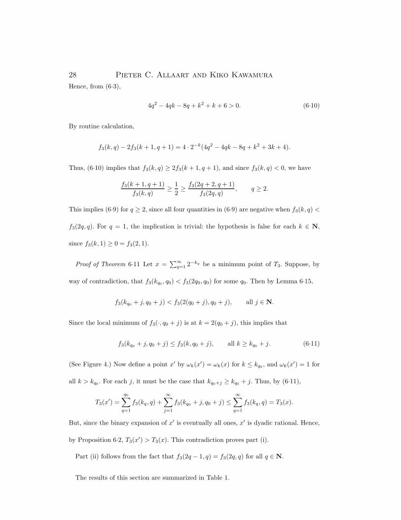
Proof of Theorem 6·11 Let x =∑∞
q=1 2−kq be a minimum point of T3. Suppose, by
way of contradiction, that f3(kq0 , q0) < f3(2q0, q0) for some q0. Then by Lemma 6·15,
f3(kq0 + j, q0 + j) < f3(2(q0 + j), q0 + j), all j ∈ N.
Since the local minimum of f3(·, q0 + j) is at k = 2(q0 + j), this implies that
f3(kq0 + j, q0 + j) ≤ f3(k, q0 + j), all k ≥ kq0 + j. (6·11)
(See Figure 4.) Now define a point x′ by ωk(x′) = ωk(x) for k ≤ kq0 , and ωk(x′) = 1 for
all k > kq0 . For each j, it must be the case that kq0+j ≥ kq0 + j. Thus, by (6·11),
T3(x′) =q0∑
q=1
f3(kq, q) +∞∑
j=1
f3(kq0 + j, q0 + j) ≤∞∑
q=1
f3(kq, q) = T3(x).
But, since the binary expansion of x′ is eventually all ones, x′ is dyadic rational. Hence,
by Proposition 6·2, T3(x′) > T3(x). This contradiction proves part (i).
Part (ii) follows from the fact that f3(2q − 1, q) = f3(2q, q) for all q ∈ N.
The results of this section are summarized in Table 1.
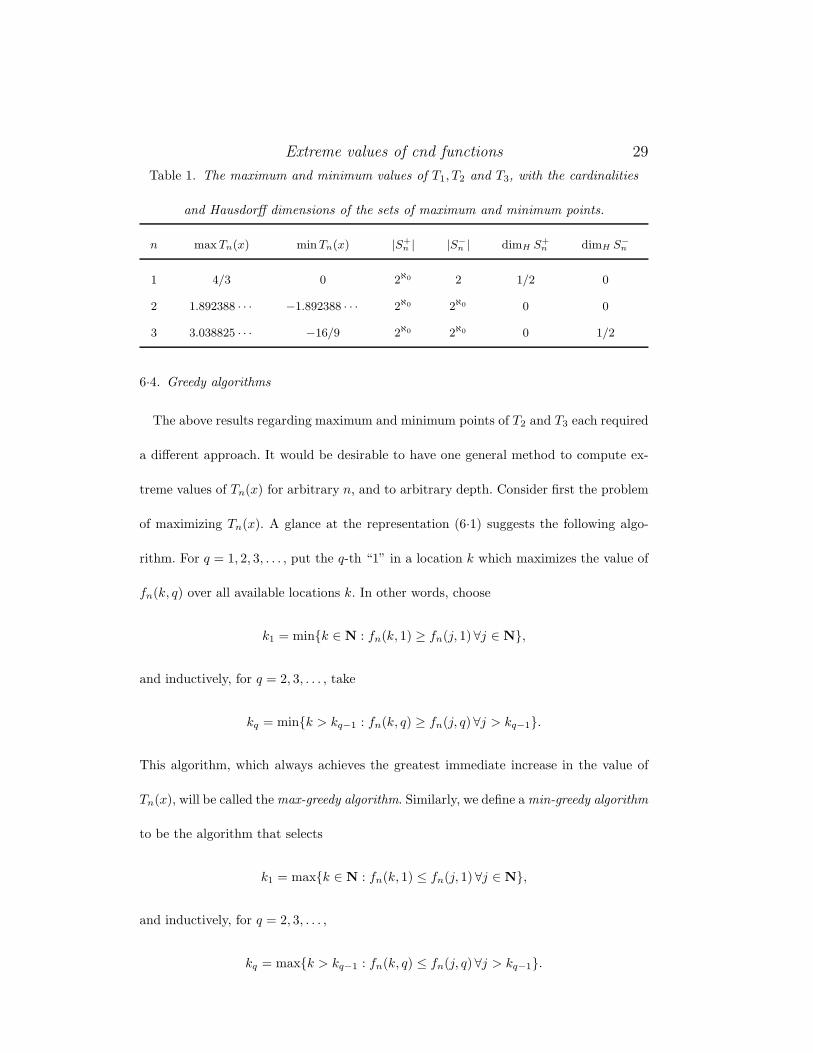
Extreme values of cnd functions 29
Table 1. The maximum and minimum values of T1, T2 and T3, with the cardinalities
and Hausdorff dimensions of the sets of maximum and minimum points.
n maxTn(x) minTn(x) |S+n | |S−
n | dimH S+n dimH S−
n
1 4/3 0 2ℵ0 2 1/2 0
2 1.892388 · · · −1.892388 · · · 2ℵ0 2ℵ0 0 0
3 3.038825 · · · −16/9 2ℵ0 2ℵ0 0 1/2
6·4. Greedy algorithms
The above results regarding maximum and minimum points of T2 and T3 each required
a different approach. It would be desirable to have one general method to compute ex-
treme values of Tn(x) for arbitrary n, and to arbitrary depth. Consider first the problem
of maximizing Tn(x). A glance at the representation (6·1) suggests the following algo-
rithm. For q = 1, 2, 3, . . . , put the q-th “1” in a location k which maximizes the value of
fn(k, q) over all available locations k. In other words, choose
k1 = min{k ∈ N : fn(k, 1) ≥ fn(j, 1)∀j ∈ N},
and inductively, for q = 2, 3, . . . , take
kq = min{k > kq−1 : fn(k, q) ≥ fn(j, q)∀j > kq−1}.
This algorithm, which always achieves the greatest immediate increase in the value of
Tn(x), will be called the max-greedy algorithm. Similarly, we define a min-greedy algorithm
to be the algorithm that selects
k1 = max{k ∈ N : fn(k, 1) ≤ fn(j, 1)∀j ∈ N},
and inductively, for q = 2, 3, . . . ,
kq = max{k > kq−1 : fn(k, q) ≤ fn(j, q)∀j > kq−1}.
30 Pieter C. Allaart and Kiko Kawamura
Heuristically, the min-greedy algorithm produces a “small” value of Tn(x). Note that
while the max-greedy algorithm chooses the smallest index in case of a tie, the min-greedy
algorithm chooses the largest index. This distinction will simplify the presentation of our
results.
We say the max-greedy algorithm is optimal for Tn if the resulting point x =∑∞
q=1 2−kq
is a maximum point of Tn. Optimality of the min-greedy algorithm is defined analogously.
Our goal is to show that the two greedy algorithms are optimal for both T2 and T3. (That
this is not clear a priori follows from the fact that the greedy algorithms can usually not
select the overall extrema of the functions fn(k, q).) Note that the max-greedy algorithm
is clearly optimal for T1.
Lemma 6·16. (a) When n = 2, the max-greedy algorithm selects kq = k+2 (q), and the
min-greedy algorithm selects kq = k−2 (q).
(b) When n = 3, the max-greedy algorithm selects kq = k+3 (q), and the min-greedy
algorithm selects kq = 2q.
Proof. First, let n = 2. That the min-greedy algorithm selects kq = k−2 (q) is obvious,
so we need only consider the max-greedy algorithm. Note that f2(k, 1) =(
12
)k−2 (k2
),
which for k ≥ 1 is maximized at k = k+2 (1). Now let q ∈ N, and suppose the max-greedy
algorithm has selected kq = k+2 (q). Clearly, the choice kq+1 = k+
2 (q+1) is available. Note
also that it is not possible to choose kq+1 to the left of the leftmost root of f2(·, q + 1).
Thus (see Figure 3), the max-greedy algorithm selects kq+1 = k+2 (q + 1).
Similar arguments apply to the proof of part (b).
Proposition 6·17. The sequences {k+n (q)}q∈N and {k−n (q)}q∈N form a partition of
N, both for n = 2 and for n = 3.
Extreme values of cnd functions 31
Proof. Note that from the proofs of Lemmas 6·4 and 6·5, we have the representations
k+2 (q) = max{k : f2(k, q + 1) < 0},
k−2 (q) = min{k : f2(k + 1, q + 1) < 0},
k+3 (q) = max{k : f3(k, q + 1) < 0}, (6·12)
k−3 (q) = min{k : f3(k + 1, q + 1) > 0}. (6·13)
We prove the proposition for n = 3. The argument for n = 2 is similar.
a) Disjointness. Let k ∈ N, and suppose, by way of contradiction, that there exist q1
and q2 such that k = k+3 (q1) = k−3 (q2). Note that this implies
2q1 < k < 2q2. (6·14)
From (6·12) and (6·13) it follows that f3(k, q1 + 1) < 0, and f3(k, q2 + 1) ≤ 0. By (6·14)
and the expansion
f3(k, q + 1) = 6−12−(k−3)(k − 2q)[k2 − (4q + 3)k + 4q2 + 2],
it follows that
k2 − (4q1 + 3)k + 4q21 + 2 < 0,
k2 − (4q2 + 3)k + 4q22 + 2 ≥ 0.
Subtracting these inequalities gives 4(q2 − q1){k − (q1 + q2)} < 0, and so
k − (q1 + q2) < 0. (6·15)
On the other hand, using (6·12) and (6·13) with the roles of q1 and q2 interchanged
yields that f3(k + 1, q1 + 1) ≥ 0 and f3(k + 1, q2 + 1) > 0. In view of (6·14), it follows
32 Pieter C. Allaart and Kiko Kawamura
that
k2 − (4q1 + 1)k + 4q21 − 4q1 ≥ 0,
k2 − (4q2 + 1)k + 4q22 − 4q2 < 0.
Subtracting these inequalities gives 4(q2 − q1){k − (q1 + q2) + 1} > 0, and so
k − (q1 + q2) + 1 > 0. (6·16)
However, since k − (q1 + q2) is integer, (6·15) and (6·16) contradict each other. Hence,
the sequences {k+3 (q)} and {k−3 (q)} are disjoint.
b) Covering. Recall from (6·7) that
k−3 (q + 1) − k−3 (q) ∈ {1, 2}, q ∈ N. (6·17)
Similarly, by rewriting the difference t+(q + 1) − t+(q), it can be seen that
k+3 (q + 1) − k+
3 (q) ∈ {2, 3}, q ∈ N. (6·18)
Observe that k−3 (q) = q for q ∈ {1, 2, 3, 4}, and k+3 (1) = 5. It is now easy to see, using
(6·17), (6·18) and the already established disjointness, that {k+3 (q)}q∈N and {k−3 (q)}q∈N
together cover N. The details are left to the interested reader.
Theorem 6·18. The max-greedy algorithm attains the maxima of T2 and T3. The
min-greedy algorithm attains the minima of T2 and T3.
Proof. By Proposition 6·17, we have
x =∞∑
q=1
2−k+n (q) =⇒ 1 − x =
∞∑q=1
2−k−n (q) (n = 2, 3).
The theorem now follows from Lemma 6·16 and Theorems 6·6, 6·9 and 6·11, using the
appropriate type of symmetry in each case.
Extreme values of cnd functions 33
6·5. Local extrema.
So far, we have only considered absolute maxima and minima of Tn. What can be said
about local extrema? How large are the sets of local maximum and minimum points of Tn?
This subsection provides some answers. First, we show how a dense set of local extreme
points of Tn can be obtained using the binary expansion of any global extreme point.
Then we give a complete characterization of the sets of local maximum and minimum
points of T2 and T3.
Definition 6·19. Let x and x′ be points in (0, 1). We say that x is a finite binary
shuffle of x′ if there exists a positive integer K such that qk(x) = qk(x′) for all k ≥ K.
Thus, x is a finite binary shuffle of x′ if and only if x can be obtained from x′ by
rearranging the first K binary digits of x′. Note that this condition is stronger than the
condition “the binary expansions of x and x′ agree beyond some index K”.
Kahane [4] proved that the local minimum points of T1 are exactly the dyadic rationals,
and the local maximum points are exactly those points x = .ω1ω2 · · · satisfying ω1 +ω2+
· · ·+ ω2k = k, for all large enough k. In our terminology, the last condition is equivalent
to x being a finite binary shuffle of a global maximum point of T1. Generalizing this idea,
we obtain a sufficient condition for a point x to be a local maximum point of Tn.
Theorem 6·20. Let x ∈ (0, 1). If x is a finite binary shuffle of some global maximum
(minimum) point x′ of Tn, then x is a local maximum (minimum) point of Tn.
Proof. Let x be a finite binary shuffle of a global maximum point x′ of Tn, and let K
be the number from Definition 6·19. Suppose that x is not a local maximum point of Tn.
Since the binary expansion of x eventually matches that of x′, it is non-terminating by
Proposition 6·2. Thus, there exists a point y whose first K binary places match those of
34 Pieter C. Allaart and Kiko Kawamura
x, such that Tn(y) > Tn(x). This implies that
∞∑k=K+1
ωk(y)fn(k, qk(y)) >∞∑
k=K+1
ωk(x)fn(k, qk(x)). (6·19)
Define a point y′ by
ωk(y′) =
ωk(x′), k ≤ K,
ωk(y), k > K.
It is not difficult to see that qK(y′) = qK(x′) = qK(x) = qK(y), and therefore, qk(y′) =
qk(y) for all k > K. Thus, by (6·19),
Tn(y′) =K∑
k=1
ωk(y′)fn(k, qk(y′)) +∞∑
k=K+1
ωk(y′)fn(k, qk(y′))
=K∑
k=1
ωk(x′)fn(k, qk(x′)) +∞∑
k=K+1
ωk(y)fn(k, qk(y))
>
K∑k=1
ωk(x′)fn(k, qk(x′)) +∞∑
k=K+1
ωk(x)fn(k, qk(x))
= Tn(x′),
contradicting the assumption that x′ is a global maximum point of Tn. The argument
for local minima is similar.
As a consequence, the sets of local maximum (or minimum) points of Tn are dense
in [0, 1] for every n. When n equals 2 or 3, a stronger statement holds: every interval
contains uncountably many local maximum and minimum points (at least one for each
global maximum or minimum point).
The condition in Theorem 6·20 is not always necessary, as the next result shows.
Theorem 6·21. T2 has a local minimum at x = 0, and a local maximum at x = 1.
Proof. For k ∈ N, let m(k) = min{T2(x) : 2−k ≤ x ≤ 2−(k−1)}. We will show that
Extreme values of cnd functions 35
m(k) ≥ 0 for all sufficiently large k. Fix k, and let x ∈ [2−k, 2−(k−1)] be a point such
that T2(x) = m(k). If x = 2−(k−1), then T2(x) = f2(k − 1, 1), which is positive for all
sufficiently large k. Assume therefore that x < 2−(k−1), so that in the representation
x =∑∞
q=1 2−kq , we have k1 = k.
For q ∈ N, let k(q) = 2q − 32 + 1
2
√8q − 7, the rightmost root of f2(·, q). Define q =
min{q : k + q − 1 < k(q)}. Then q <∞, and f2(kq, q) ≥ 0 for all q < q. When k is large
enough, we have
3k4
≤ q ≤ k. (6·20)
We will now construct a lower bound for the sum∑∞
q=q f2(kq, q), which contains all of
the negative terms in the series∑∞
q=1 f2(kq, q), if any are present.
Using (6·2), and by considering the minimum of the polynomial t2−(4q−3)t+4(q−1)2,
we find that
f2(k, q) ≥ 2−(k−1)(−2q + 7/4), q ∈ N, k ≥ q. (6·21)
By choosing k large enough, we can ensure that q is sufficiently large so that k−2 (q) ≥
3q/2 + 1 for all q ≥ q. By (6·21), it follows that for q ≥ q,
f2(kq, q) ≥ f2(k−2 (q), q) ≥ 2−(k−2 (q)−1)(−2q + 7/4) ≥ 2−3q/2(−2q + 7/4),
where the last inequality follows since −2q + 7/4 < 0. Hence,
∞∑q=q
f2(kq , q) ≥∞∑
q=q
2−3q/2(−2q + 7/4) = −2−3q/2(Aq +B),
where A and B are calculable constants, with A > 0. Note that 3q/2 ≥ 9k/8 by (6·20),
so that f2(k, 1) = 2−(k−1)(k2 − k) > 2−3q/2(Aq +B) for all large enough k. Therefore,
m(k) =∞∑
q=1
f2(kq, q) ≥ f2(k, 1) +∞∑
q=q
f2(kq , q) > 0,
36 Pieter C. Allaart and Kiko Kawamura
for all sufficiently large k. This implies that T2 has a local minimum at x = 0. The local
maximum at x = 1 follows by symmetry.
Theorem 6·22. A point x ∈ (0, 1) is a local maximum (minimum) point of T2 if and
only if x is a finite binary shuffle of some global maximum (minimum) point of T2.
Proof. We need only prove the “forward” direction of the theorem, and do so first for
minima. Let x ∈ (0, 1) be a local minimum point of T2. For q ∈ N, let M(q) be the set
of all indices k that minimize f2(k, q). That is, M(q) = {k−2 (q) − 1, k−2 (q)} if 8q + 1 is
square, and M(q) = {k−2 (q)} otherwise.
Note first that x cannot be dyadic rational, for if it were, then the proof of Theorem
5·1 would imply that T2(x−2−m) < T2(x) < T2(x+2−m) for all large enough m. Hence,
there exists a dyadic interval I = [r/2l, (r + 1)/2l], such that T2 attains its absolute
minimum over I at x, and x is interior to I.
Since T2(x) ≤ T2(r/2l), there is an index k0 > l with ωk0(x) = 1 and f2(k0, qk0(x)) ≤ 0.
Let q0 := qk0(x), so that kq0 = k0. Define the number
j∗ := min{j : k0 + j ≤ k−2 (q0 + j)}.
Note that j∗ is finite since k−2 (q) increases in steps of 2 for infinitely many q. Now for
1 ≤ j < j∗, k0 + j is to the right of k−2 (q0 + j), and on or to the left of the rightmost root
of f2(·, q0 + j). (Since this is true for j = 0 by the assumption f2(k0, q0) ≤ 0 (see Figure
3), and the rightmost root of f2(·, q) increases by at least 1 for each q.) It follows that
f2(k0 + j, q0 + j) ≤ f2(k, q0 + j), 1 ≤ j < j∗, k ≥ k0 + j.
Since kq0+j ≥ k0 + j for all j, we obtain
∑q>q0
f2(kq, q) ≥j∗−1∑j=1
f2(k0 + j, q0 + j) +∞∑
j=j∗f2(k−2 (q0 + j), q0 + j),
Extreme values of cnd functions 37
with equality if and only if kq0+j = k0 + j for all 1 ≤ j < j∗, and kq0+j ∈ M(q0 + j) for
all j ≥ j∗. But then, by Theorem 6·6, x is a finite binary shuffle of some global minimum
point.
Next, let x be a local maximum point of T2. Then 1 − x is a local minimum point,
whose binary expansion is obtained from that of x by complementation. From the above
proof, it follows that 1−x is a finite binary shuffle of some global minimum point 1−x′.
But then x is also a finite binary shuffle of x′, and since x′ is a global maximum point of
T2, the proof of the theorem is complete.
A similar result holds for the local maxima of T3, though for this case, the argument
is slightly more subtle.
Theorem 6·23. A point x is a local maximum point of T3 if and only if x is a finite
binary shuffle of some global maximum point of T3.
The proof uses the following sets, defined for q ∈ N. If 24q+1 is a square, let M+(q) =
{k+3 (q), k+
3 (q) + 1} and M−(q) = {k−3 (q) − 1, k−3 (q)}. Otherwise, let M+(q) = {k+3 (q)}
and M−(q) = {k−3 (q)}.
Proof of Theorem 6·23 Let x be a local maximum point of T3. Then there exists a
dyadic interval I = [r/2l, (r + 1)/2l], such that T3 attains its absolute maximum over I
at x. As in the proof of Theorem 6·22, x is dyadic irrational. We can therefore choose
the interval I small enough so that q0 := ql(x) ≥ 3.
Now consider two cases. First, suppose that kq := kq(x) ≥ 2(q−1) for all q > q0. Then
it follows immediately that
∑q>q0
f3(kq, q) ≤∑q>q0
f3(k+3 (q), q), (6·22)
38 Pieter C. Allaart and Kiko Kawamura
with equality if and only if kq ∈ M+(q) for all q > q0. By the results of the previous
subsection, x must be a finite binary shuffle of some global maximum point of T3.
Next, suppose that kq < 2(q − 1) for at least one q > q0. Fix this value of q. Now for
each j ∈ N, we must have kq+j ≥ kq + j. And, by a repeated application of Lemma 6·14,
f3(kq + j, q + j) > f3(k+3 (q + j), q + j), (6·23)
as long as kq + j ≥ k−3 (q + j). Thus, the only way for x to be an absolute maximum
point over I given the condition kq < 2(q − 1), is that kq+j = kq + j for all j with
kq + j ≥ k−3 (q + j), and kq+j ∈ M−(q + j) for all other j. But in view of Theorem 6·9,
this implies x is a finite binary shuffle of some global maximum point of T3.
Theorem 6·24. A point x ∈ [0, 1] is a local minimum point of T3 if and only if x is
either a dyadic rational, or a finite binary shuffle of some global minimum point of T3.
Proof. If x is a local minimum point of T3, then it must be an absolute minimum point
over some dyadic interval. By essentially the same argument as in the proof of Theorem
6·11, it follows that either (a) the binary expansion of x is eventually all ones, in which
case x is dyadic rational; or (b) the binary expansion of x satisfies kq ∈ {2q−1, 2q} for all
q beyond some index, in which case x is a finite binary shuffle of some global minimum
point of T3.
Conversely, let x0 be any dyadic rational, and let q0 denote the number of ones in the
binary expansion of x0. We will show that
T3(x0) = min{T3(x) : x0 ≤ x ≤ x0 + δ}, for some δ > 0. (6·24)
Applying the same argument to the point 1 − x0, and using the line symmetry of the
graph of T3, then yields that T3 has a local minimum at x0.
Extreme values of cnd functions 39
For k ∈ N, let Ik = [x0 + 2−k, x0 + 2−(k−1)], and let m(k) = min{T3(x) : x ∈ Ik}. We
may assume that k is large enough so that if x0 = j/2l in lowest terms, then k > l+1. If
the minimum value of T3 over Ik is taken on at one of the endpoints, then m(k)−T3(x0)
is either f3(k − 1, q0 + 1) or f3(k, q0 + 1), and so m(k) ≥ T3(x0) for sufficiently large k.
Otherwise, the argument from the second part of the proof of Proposition 6·2 implies
that the minimum over Ik is attained at some dyadic irrational point x =∑∞
q=1 2−kq .
For q ∈ N, let k(q) = 2q − 12 + 1
2
√24q − 23, the rightmost root of f3(·, q). Assume
k ≥ k(q0 + 1), and let q = min{q : k + q − q0 − 1 < k(q)}. Then q0 + 1 < q < ∞, and
f3(kq, q) ≥ 0 for all q0 < q < q. By choosing k large enough, we can further ensure that
q ≥ 23 (k − q0).
Since x is dyadic irrational, the proof of Theorem 6·11 shows that f3(kq, q) ≥ f3(2q, q)
for all q ≥ q. Thus,
∞∑q=q
f3(kq, q) ≥∞∑
q=q
f3(2q, q) = −∞∑
q=q
4−(q−2)(q − 1) = −(64/9)2−2q(3q − 2).
Since q ≥ 23 (k − q0), the magnitude of the last expression goes to zero faster than
f3(k, q0 + 1) as k → ∞. Hence, for all sufficiently large k,
T3(x) − T3(x0) =∑q>q0
f3(kq, q) ≥ f3(k, q0 + 1) +∞∑
q=q
f3(kq , q) > 0,
and so m(k) > T3(x0). This implies (6·24).
6·6. Results and conjectures for the extrema of Tn
Proposition 6·25. For every n ≥ 2,
2n
√πn
∼(
12
)n(2nn
)< max
0≤x≤1Tn(x) < 2n−1.
Proof. The lower bound follows since
max0≤x≤1
Tn(x) > Tn(2−2n) = fn(2n, 1) =(
12
)n(2nn
).
40 Pieter C. Allaart and Kiko Kawamura
By Stirling’s formula,(
12
)n (2nn
) ∼ 2n/√πn as n→ ∞.
To see the upper bound, let Mn := max0≤x≤1 |Tn(x)|, and note that by (2·3),
|Tn(x)| ≤ 12Mn +Mn−1, 0 ≤ x ≤ 1, n ≥ 2.
It follows that Mn ≤ 2Mn−1. By Theorem 6·6 and Corollary 6·7, we have M2 < 2 and,
hence, Mn < 2n−1 for all n ≥ 2.
Conjecture A.
(i) The max-greedy algorithm is optimal for Tn, for all n ∈ N.
(ii) The min-greedy algorithm is optimal for T2n−1, for all n ∈ N.
Conjecture A is based not only on the fact that the greedy algorithms are optimal
for T1, T2 and T3, but also on extensive numerical experimentation. (The min-greedy
algorithm does not appear to be optimal for Tn when n is even and n > 2. Of course,
in this case the minimum is directly related to the maximum, via the point-symmetry of
the graph of Tn.)
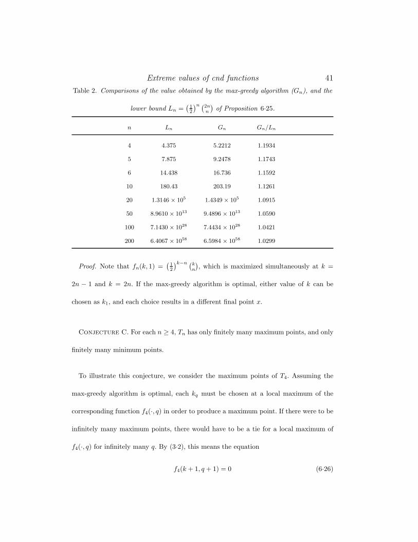
Table 2 shows the values obtained by the max-greedy algorithm (Gn), as well as the
lower bound from Proposition 6·25 (Ln). The last column gives the ratio of these values,
which seems to tend to 1 as n→ ∞. This suggests the following guess.
Conjecture B. As n→ ∞,
max0≤x≤1
Tn(x) ∼ 2n
√πn
. (6·25)
Lastly, we address the number of maximum and minimum points of Tn.
Proposition 6·26. Let n ∈ N. Provided the max-greedy algorithm is optimal for Tn,
Tn has at least two distinct maximum points in the interval [0, 12 ].
Extreme values of cnd functions 41
Table 2. Comparisons of the value obtained by the max-greedy algorithm (Gn), and the
lower bound Ln =(
12
)n (2nn
)of Proposition 6·25.
n Ln Gn Gn/Ln
4 4.375 5.2212 1.1934
5 7.875 9.2478 1.1743
6 14.438 16.736 1.1592
10 180.43 203.19 1.1261
20 1.3146 × 10⁵ 1.4349 × 10⁵ 1.0915
50 8.9610 × 10¹³ 9.4896 × 10¹³ 1.0590
100 7.1430 × 1028 7.4434 × 1028 1.0421
200 6.4067 × 1058 6.5984 × 1058 1.0299
Proof. Note that fn(k, 1) =(
12
)k−n (kn
), which is maximized simultaneously at k =
2n − 1 and k = 2n. If the max-greedy algorithm is optimal, either value of k can be
chosen as k1, and each choice results in a different final point x.
Conjecture C. For each n ≥ 4, Tn has only finitely many maximum points, and only
finitely many minimum points.
To illustrate this conjecture, we consider the maximum points of T4. Assuming the
max-greedy algorithm is optimal, each kq must be chosen at a local maximum of the
corresponding function f4(·, q) in order to produce a maximum point. If there were to be
infinitely many maximum points, there would have to be a tie for a local maximum of
f4(·, q) for infinitely many q. By (3·2), this means the equation
f4(k + 1, q + 1) = 0 (6·26)
42 Pieter C. Allaart and Kiko Kawamura
would have to have infinitely many integer solutions. Setting p := k − q + 1, (6·26) can
be written as∑4
i=0(−1)i(pi
)(q
4−i
)= 0, and the further substitution x = p− q, y = p+ q
transforms this into
x4 − 6x2y + 8x2 + 3y2 − 6y = 0, (6·27)
or equivalently,
z2 − 6zy + 3y2 + 8z − 6y = 0, (6·28)
z = x2.
Equation (6·28) does have infinitely many integer solutions (z, y), and they can be found
by a standard method [6, Chapter 11]. For m ∈ Z, let
um = ±12
{(4 +
√6)(5 + 2
√6)m + (4 −
√6)(5 − 2
√6)m},
vm = ± 12√
6
{(4 +
√6)(5 + 2
√6)m − (4 −
√6)(5 − 2
√6)m},
(6·29)
where the signs of um and vm are independent. Then
(z, y) =(um + 3vm + 1
2,vm + 3
2
)(6·30)
is an integer solution to (6·28), and conversely, each solution to (6·28) must be of the form
(6·30). The question is, for how many of these solutions z is a square. An exhaustive com-
puter search showed that the only solution pairs (6·30) with |m| ≤ 1000 (and any choice
of signs in (6·29)) for which z is a square in fact have |m| ≤ 5. They are (0, 0), (0, 2),
(1, 1), (1, 3), (4, 2), (4, 8), (9, 3), (9, 17), (36, 8), (36, 66), (8281, 1521) and (8281, 15043).
We guess therefore that (6·27) has only finitely many integer solutions. Numerical com-
putations also indicate that only two of the above solution pairs (z, y) correspond to a
pair (k, q) such that the max-greedy algorithm selects kq = k. These are (36, 8) (corre-
Extreme values of cnd functions 43
sponding to k = 7, q = 1) and (8281, 1521) (corresponding to k = 1520, q = 715). Thus,
it seems as though T4 has precisely 4 distinct maximum points.
Finally, we point out that, while the minimum of T3(x) was attained by choosing
kq = 2q − 1 or kq = 2q for each q, this sequence does not work for higher-indexed Tn’s,
even though the function fn(·, q) has a local extremum at 2q for every odd n. For instance,
when n = 5, f5(·, q) has in fact a local maximum at 2q. For n = 7, f7(·, q) does have a local
minimum at 2q, but an easy calculation shows that∑∞
q=1 f7(2q, q) = −256/81 > −4,
whereas f7(10, 2) = −6.
Acknowledgements. We wish to express our gratitude to Prof. R. D. Mauldin for many
valuable comments and suggestions.
REFERENCES
[1] K. J. Falconer, The geometry of fractal sets. Cambridge University Press (1985).
[2] M. Hata and M. Yamaguti, Takagi function and its generalization, Japan J. Appl. Math.,
1, pp. 183-199 (1984).
[3] H. Kairies, Takagi’s function and its functional equations, Rocznik Nauk.-Dydakt. Prace
Mat., 15, pp. 73-83 (1998).
[4] J-P. Kahane, Sur l’exemple, donne par M. de Rham, d’une fonction continue sans derivee,
Enseignement Math. 5, pp. 53-57 (1959).
[5] K. Kawamura, On the classification of self-similar sets determined by two contractions on
the plane, J. Math. Kyoto Univ. 42, pp. 255-286 (2002).
[6] H. L. Keng, Introduction to number theory, (Translated from the Chinese original by Peter
Shiu) Springer Verlag, Berlin Heidelberg New York (1982).
[7] N. Kono, On self-affine functions, Japan J. Appl. Math. 3, pp. 259-269 (1986).
[8] N. Kono, On generalized Takagi functions, Acta Math. Hungar. 49, pp. 315-324 (1987).
44 Pieter C. Allaart and Kiko Kawamura
[9] Z. Lomnicki and S. Ulam, Sur la theorie de la mesure dans les espaces combinatoires et
son application au calcul des probabilites I. Variables independantes. Fund. Math. 23,
pp. 237-278 (1934).
[10] R. Mauldin and S. Williams, On the Hausdorff dimension of some graphs, Trans. Amer.
Math. Soc. 298, pp. 793-803 (1986).
[11] T. Okada, T. Sekiguchi and Y. Shiota, Applications of binomial measures to power
sums of digital sums, J. Number Theory 52, pp. 256-266 (1995).
[12] T. Okada, T. Sekiguchi and Y. Shiota, An explicit formula of the exponential sums of
digital sums, Japan J. Indust. Appl. Math. 12, pp. 425-438 (1995).
[13] G. de Rham, Sur quelques courbes definies par des equations fonctionnelles, Rend. Sem.
Mat. Torino, 16, pp. 101-113 (1957).
[14] T. Sekiguchi and Y. Shiota, A generalization of Hata-Yamaguti’s results on the Takagi
function, Japan J. Appl. Math. 8, pp. 203-219 (1991).
[15] T. Takagi, A simple example of the continuous function without derivative, The Collected
Papers of Teiji Takagi, Iwanami Shoten Pub., pp. 5-6 (1973).
[16] S. Tasaki, I. Antoniou and Z. Suchanecki, Deterministic diffusion, De Rham equation
and fractal eigenvectors, Physics Letter A 179, pp. 97-102 (1993).
[17] M. Urbanski, The Hausdorff dimension of the graphs of continuous self-affine functions,
Proc. Amer. Math. Soc. 108, pp. 921-930 (1990).
[18] M. Yamaguti and M. Hata, Weierstrass’s function and chaos, Hokkaido Math. J. 12,
pp. 333-342 (1983).


![Continuous Nowhere Differentiable Functions · 2017-10-10 · M. Lynch 1992 62 Example based on topology B. R. Hunt 1994 78 ND[0,1] is a prevalent set L. Wen 2002 64 Example based](https://img.pdfslide.us/doc/110x75/5e913eef72956b41317768b9/continuous-nowhere-differentiable-functions-2017-10-10-m-lynch-1992-62-example.jpg)


![[Hitchin N.] Differentiable Manifolds(BookZZ.org)](https://img.pdfslide.us/doc/110x75/55cf903b550346703ba416cf/hitchin-n-differentiable-manifoldsbookzzorg.jpg)