1 Exploring Context with Deep Structured models for ... Exploring Context with Deep Structured models for Semantic Segmentation Guosheng Lin, Chunhua Shen, Anton van den Hengel, Ian

APPEARING IN IEEE TRANSACTIONS ON PATTERN ANALYSIS AND MACHINE INTELLIGENCE, APRIL 2017. 1

Exploring Context with Deep Structured modelsfor Semantic Segmentation

Guosheng Lin, Chunhua Shen, Anton van den Hengel, Ian Reid

Abstract—State-of-the-art semantic image segmentation methods are mostly based on training deep convolutional neural networks(CNNs). In this work, we proffer to improve semantic segmentation with the use of contextual information. In particular, we explorepatch-patch context and patch-background context in deep CNNs. We formulate deep structured models by combining CNNs andConditional Random Fields (CRFs) for learning the patch-patch context between image regions. Specifically, we formulate CNN-basedpairwise potential functions to capture semantic correlations between neighboring patches. Efficient piecewise training of the proposeddeep structured model is then applied in order to avoid repeated expensive CRF inference during the course of back propagation.Forcapturing the patch-background context, we show that a network design with traditional multi-scale image inputs and sliding pyramidpooling is very effective for improving performance. We perform comprehensive evaluation of the proposed method. We achieve newstate-of-the-art performance on a number of challenging semantic segmentation datasets.

Index Terms—Semantic Segmentation, Convolutional Neural Networks, Conditional Random Fields, Contextual Models

F

CONTENTS

1 Introduction 21.1 Related work . . . . . . . . . . . . . . . 2

2 Modeling semantic pairwise relations 3

3 Contextual Deep CRFs 43.1 Unary potential functions . . . . . . . . 43.2 Pairwise potential functions . . . . . . . 4

3.2.1 Asymmetric pairwise poten-tials . . . . . . . . . . . . . . . 5

4 Exploring background context 6

5 Network configurations 6

6 Prediction 76.1 Coarse-level prediction stage . . . . . . 76.2 Prediction refinement stage . . . . . . . 8

7 CRF training 87.1 Piecewise training of CRFs . . . . . . . . 8

8 Implementation details 98.1 Efficient learning . . . . . . . . . . . . . 98.2 Asynchronous gradient update . . . . . 9

• G. Lin is with School of Computer Science and Engineering, NanyangTechnological University, Singapore. This work was done when G. Linwas with The University of Adelaide and Australian Centre for RoboticVision. E-mail: [email protected]. Shen, A. van den Hengel and I. Reid are with School of Com-puter Science, The University of Adelaide, Australia; and AustralianCentre for Robotic Vision. E-mail: {chunhua.shen, anton.vandenhengel,ian.reid}@adelaide.edu.au

• C. Shen is the corresponding author.

9 Experiments 109.1 Results on the NYUDv2 dataset . . . . . 10

9.1.1 Component evaluation . . . . 119.1.2 Comparison with multi-

unary ensemble . . . . . . . . 119.2 Results on the PASCAL VOC 2012 dataset 129.3 Results on the Cityscapes dataset . . . . 129.4 Results on the PASCAL-Context dataset 129.5 Results on the SUN-RGBD dataset . . . 139.6 Results on the COCO dataset . . . . . . 139.7 Results on the SIFT-flow dataset . . . . . 139.8 Results on the KITTI dataset . . . . . . . 14

10 Conclusions 14

References 14

arX

iv:1

603.

0318

3v3

[cs

.CV

] 2

May

201

7


1 INTRODUCTION

Semantic image segmentation aims to predict a categorylabel for every image pixel, which is an important yet chal-lenging task for image understanding. Recent approacheshave applied convolutional neural network (CNNs) [5], [17],[39] to this pixel-level labeling task and achieved remarkablesuccess. Among these CNN-based methods, fully convolu-tional neural networks (FCNNs) [5], [39] have become apopular choice, because of their computational efficiency fordense prediction and end-to-end style learning.

Contextual relationships are ubiquitous and provide im-portant cues for scene understanding tasks. Spatial contextcan be formulated in terms of semantic compatibility re-lations between one object and its neighboring objects orimage patches (stuff), in which a compatibility relation isan indication of the co-occurrence of visual patterns. Forexample, a car is likely to appear over a road, and a glassis likely to appear over a table. Context can also encodeincompatibility relations. For example, a boat is unlikely toappear on a road. These relations also exist at finer scales,for example, in object part-to-part relations, and part-to-object relations. In some cases, contextual information is themost important cue, particularly when a single object showssignificant visual ambiguities. A more detailed discussion ofthe value of spatial context can be found in [26].

We explore two types of spatial context to improve thesegmentation performance: patch-patch context and patch-background context. The patch-patch context is the semanticrelation between the visual patterns of two image patches.Likewise, patch-background context the semantic relationbetween an image patch and a large background region.

Explicitly modeling the patch-patch contextual relationshas not been well studied in recent CNN-based segmenta-tion methods. In this work, we propose to explicitly modelthe contextual relations using conditional random fields(CRFs). We formulate CNN-based pairwise potential func-tions to capture semantic correlations between neighboringpatches. Some recent methods combine CNNs and CRFsfor semantic segmentation, e.g., the dense CRFs appliedin [5], [8], [48], [60]. The purpose of applying the denseCRFs in these methods is to refine the upsampled low-resolution prediction to sharpen object/region boundaries.These methods consider Potts-model-based pairwise po-tentials for enforcing local smoothness. There the pairwisepotentials are conventional log-linear functions. In contrast,here we learn more general pairwise potentials using CNNsto model the semantic compatibility between image re-gions. Our CNN pairwise potentials aim to improve thecoarse-level prediction rather than merely encouraging localsmoothness, and thus have a different purpose comparedto Potts-model-based pairwise potentials. Given that thesetwo types of potentials make different effects, they can becombined to improve segmentation results. Fig. 1 illustratesthe prediction process of our method.

In contrast to patch-patch context, patch-backgroundcontext is widely explored in the literature. For CNN-based methods, background information can be effectivelycaptured by combining features from a multi-scale im-age network input, and has shown good performance insome recent segmentation methods [17], [40]. A special

case of capturing patch-background context is consideringthe whole image as the background region and incorpo-rating the image-level label information into learning. Inour approach, to encode rich background information, weconstruct multi-scale networks and apply sliding pyramidpooling on feature maps. The traditional pyramid pooling(in a sliding manner) on the feature map is able to captureinformation from background regions of different sizes.

Incorporating general pairwise potentials usually in-volves computationally expensive inference, which bringschallenges for CRF learning. To facilitate efficient learningwe apply piecewise training of the CRF [53] to avoid re-peated inference during back propagation training of thedeep model.

Thus our main contributions are as follows.

• We formulate CNN-based general pairwise potentialfunctions in CRFs to explicitly model patch-patchsemantic relations.

• Deep CNN-based general pairwise potentials arechallenging for efficient CNN-CRF joint learning. Weperform approximate training, using piecewise train-ing of CRFs [53], to avoid the repeated inference atevery stochastic gradient descent iteration and thusachieve efficient learning.

• We explore background context by applying a net-work architecture with traditional multi-scale imageinput [17] and sliding pyramid pooling [31]. Weempirically demonstrate the effectiveness of this net-work architecture for semantic segmentation.

• We set new state-of-the-art performance on a num-ber of challenging semantic segmentation datasets,including NYUDv2, PASCAL VOC 2012, PASCAL-Context, SIFT-flow, SUN-RGBD, Cityscapes datasetand so on. In particular, we achieve an intersection-over-union score of 77.8 on the PASCAL VOC 2012dataset.

1.1 Related work

Preliminary results of our work appeared in [33]. Exploit-ing contextual information has been widely studied in theliterature (e.g., [11], [26], [46]). For example, early work of“TAS” [26] models different types of spatial context betweenThings and Stuff using a generative graphical model.

The most successful recent methods for semantic imagesegmentation are based on CNNs. CNN based methodshave shown outstanding performance compared to tra-ditional semantic segmentation methods like TextonBoost[49]. A number of these CNN-based methods are region-proposal-based methods [19], [24], which first generate re-gion proposals and then assign category labels to each ofthem. Very recently, FCNNs [5], [8], [39] have become apopular choice for their efficient feature generation and end-to-end training. FCNNs have also been applied to a range ofother dense-prediction tasks recently, such as image restora-tion [14], image super-resolution [12] and depth estimation[13], [15], [36]. The method that we propose here is also builtupon fully convolution-style networks.

FCNN methods make use of the Image-Net trainedCNN models (e.g., the VGG-16 model [51]) which takes


...

Pairwise potential netMulti-scale CNN

...

Unary potential net:Multi-scale CNN

Deep structured model: Contextual deep CRF

Prediction refinement stage:

Up-sample & Refine

Coarse-level prediction stage:

CRF Inference

Low-resolution prediction

Final prediction

Fig. 1 – An illustration of the prediction process of our method. Both our unary and pairwise potentials are formulated asmulti-scale CNNs for capturing semantic relations between image regions. Our method outputs low-resolution predictionafter performing CRF inference, then the prediction is up-sampled and refined in a standard post-processing stage to outputthe final prediction.

Feature map(low resolution) CRF graphConstruct CRF graph

(according to the feature map resolution)

1. Node construction: each node corresponds to each spatial position in the feature map.

2. Pairwise connections: each node connects to all nodes that lie within a pre-defined range box

FeatMap-Net

Fig. 2 – An illustration of generating a feature map with FeatMap-Net and constructing the CRF graph.

advantages of the large Image-Net dataset for learning deepmodels. For convolution and pooling layers, the resolutionof the output feature map is down-sampled if the convo-lution/pooling stride is greater than 1. Usually a few suchlayers use a stride setting of 2, hence the direct predictionsof FCNNs are typically in low resolution. To increase theprediction resolution, the naive method of directly reducingthe strides for all layers is not able to address this down-sampled prediction for a deep network. Small strides resultin prohibitively expensive computation for a deep network,and also reduce the view-of-field (the image region thata filter is able to “see”) of the network layers. Networklayers with insufficient view-of-field may not be able tocapture high-level semantic patterns and thus degrade theperformance.

To address this low-resolution prediction issue, a varietyof FCNN based methods are proposed very recently whichfocus on refining the low-resolution prediction to obtainhigh resolution prediction. DeepLab-CRF [5] first appliesatrous convolution to produce larger size feature mapsand performs bilinear upsampling on the prediction scoremap to the input image size, then they apply the denseCRF method [30] to refine the object boundary by leveringlow-level (color contrast) information. They consider Potts-model based pairwise potential functions which enforcelocal smoothness. CRF-RNN [60] extends this approach byimplementing the mean field CRF inference as recurrentlayers for end-to-end learning of the dense CRF and FCNNnetwork. The work in [42] learns deconvolution layers toupsample the low-resolution predictions. The depth esti-mation method [37] explores super-pixel pooling for build-ing the gap between the low-resolution feature map andhigh-resolution final prediction. Eigen et al. [13] performcoarse-to-fine learning of multiple networks with differentresolution outputs for refining the coarse prediction. Themethod FCN [39] and Hyper-column [23] explore mid-layerfeatures (skip connections) for high-resolution prediction.

Surrounding Above/Below

Fig. 3 – An illustration of constructing pairwise connec-tions in a CRF graph. A node is connected to all othernodes which lie inside the range box (dashed box in thefigure). Two types of spatial relations are described inthe figure, which correspond to two types of pairwisepotential functions.

Unlike these methods, our method focuses on improving thecoarse (low-resolution) prediction by learning general CNNpairwise potentials to capture semantic relations betweenpatches. These methods are complementary to our method.

Jointly learning CNNs and CRFs has also been exploredin other applications apart from segmentation. Recent workin [36], [37] proposes to jointly learn continuous CRFs andCNNs for depth estimation from single monocular images.They focus on continuously-valued variable prediction,while our method is for discrete categorical label prediction.The work in [55] combines CRFs and CNNs for humanpose estimation. The authors of [6] explore joint trainingof Markov random fields and deep neural networks for thetasks of predicting words from noisy images and multi-classclassification. They require marginal inference for everygradient calculation which is computationally expensive fortraining deep models.

2 MODELING SEMANTIC PAIRWISE RELATIONS

We first describe how to build the CRF graph for modelingsemantic pairwise relations. Given an image, we first applya convolutional network to generate a feature map. We


refer to this network as ‘FeatMap-Net’, details of which arepresented in Sec. 4 (Fig. 6 shows the overall architecture).With this feature map, we construct one node in the CRFgraph corresponding to one spatial position of the featuremap. Fig. 2 illustrates how we construct nodes and pairwiseconnections in a CRF graph.

Pairwise connections are constructed by connecting onenode to all other nodes which lie within a spatial rangebox (the dashed box in Fig. 3). We consider different spatialrelations by defining different types range boxes, and eachtype of spatial relation is modeled by a specific pairwisepotential function. As shown in Fig. 3, our method modelsthe “surrounding” and “above/below” spatial relations. Forthe surrounding relation, the range box is centered at thenode. For the above/below relation, the bottom edge of therange box is centered at the node.

In our experiments, the size of the range box (dash boxin the figure) size is 0.4a× 0.4a, where a is the length of theshort edge of the feature map. It would be straightforwardto construct more pairwise potentials, by varying either thesizes or positions of the connection range boxes, and ourapproach is not limited to connections within “boxes”.

3 CONTEXTUAL DEEP CRFS

Here we present the details of our deep CRF model. We de-note by x ∈ X one input image and y ∈ Y the labeling maskwhich describes the label configuration of each node in theCRF graph. The energy function is denoted by E(y,x;θ)which models the compatibility of the input-output pair,with a small output value indicating high confidence inthe prediction y. All network parameters are denoted byθ which we need to learn. The conditional likelihood forone image is formulated as follows:

P (y|x) = 1

Z(x)exp [−E(y,x)]. (1)

Here Z is the partition function, defined as: Z(x) =∑y exp [−E(y,x)]. The energy function is typically formu-

lated by a set of unary and pairwise potentials:

E(y,x) =∑U∈U

∑p∈NU

U(yp,xp)

+∑V ∈V

∑(p,q)∈SV

V (yp, yq,xpq). (2)

Here U is a unary potential function. To make the expo-sition more general, we consider multiple types of unarypotentials with U the set of all such unary potentials. NU isa set of nodes for the potential U . Likewise, V is a pairwisepotential function with V the set of all types of pairwisepotential. SV is the set of edges for the potential V . xp

and xpq indicates the corresponding image regions whichassociate to the specified node and edge.

The potential function is constructed by a deep networkfor generating feature map (FeatMap-Net) and a shallownetwork (Unary-Net or Pairwise-Net) to generate the outputof the potential function. Details are described in the follow-ing sections. An overview of our contextual deep structuredmodel for prediction and training is shown in Fig. 4.

3.1 Unary potential functionsWe formulate the unary potential function by stacking theFeatMap-Net for generating feature maps and a shallowerfully connected network (referred to as Unary-Net) to gen-erate the final output of the unary potential function. Theunary potential function is written as follows:

U(yp,xp;θU ) = −zp,yp(x;θU ). (3)

Here zp,ypis the output value of Unary-Net, which corre-

sponds to the p-th node and the yp-th class.Fig. 4 shows an illustration of the Unary-Net and how

it corporates with FeatMap-Net. Fig. 5 demonstrates theprocess for generating the feature vector for one node. Theinput of the Unary-Net is the node feature vector extractedfrom the feature map which is generated by FeatMap-Net.The feature vector for one CRF node is simply the corre-sponding feature vector in the feature map. The dimensionof the Unary-Net output vector for one node is K , which isthe same as the number of classes.

3.2 Pairwise potential functionsWe formulate the unary potential function, analogous to theunary potentials, by stacking the FeatMap-Net for generat-ing feature maps and a shallower fully connected network(referred to as Pairwise-Net) to generate the final outputof the pairwise potential function. The pairwise potentialfunction is written as follows:

V (yp, yq,xpq;θV ) = −zp,q,yp,yq(x;θV ). (4)

Here zp,q,yp,yqis the output value of Pairwise-Net. It is the

confidence value for the node pair (p, q) when they arelabeled with the class value (yp, yq), which measures thecompatibility of the label pair (yp, yq) given the input imagex. θV is the corresponding set of CNN parameters for thepotential V , which we need to learn. The role of Pairwise-Net in our structured model is illustrated in Fig. 4. Fig. 5describes the process for generating the feature vector forone pairwise connection. The input of Pairwise-Net is theedge feature vector which is generated from the featuremap for two connected nodes. Following the work of [29],we concatenate the corresponding feature vectors of twoconnected nodes to obtain the CRF edge feature vector. ThePairwise-Net has K2 output units to match the number ofpossible label combinations for a pair of nodes.

Our formulation of pairwise potentials is different fromthe Potts-model-based smoothness potentials in the existingmethods of [5], [60]. The Potts-model-based pairwise poten-tials are a log-linear functions and employ a special formula-tion for enforcing neighborhood smoothness based on colorcontrast, and thus to sharpen object/region boundaries.In contrast, our pairwise potentials model the semanticcompatibility relations between two nodes with the outputfor every possible value of the label pair (yp, yq) individ-ually parameterized by CNNs. Clearly, these two types ofpairwise potential formulations have different purposes andeffects.

Most recent segmentation methods, e.g., the work in [5],[8], [48], [60], have applied the dense CRF method [30] inthe prediction refinement stage for refining (sharpen ob-ject boundaries) the coarse (low-resolution) prediction. The


Edge feature vector

Feature map(low resolution)

One pairwise connection (edge)

Unary-NetNode

feature vector

One unary potential output:One node

CRF graph

Pairwise-Net

One pairiwise potential output:

Generatefeatures

Distribution of the prediction:

in which,

FeatMap-Net

Construct CRF graph(according to the feature map)

Coarse level prediction: CRF marginal inference

Prediction stage

Network parameter learning:Minimise negative log-likelihood

Learning stage

Other nodes/edges

Low resolution prediction

Fig. 4 – An overview of the proposed contextual deep structured model. Unary-Net and Pairwise-Net are shown here forgenerating potential function outputs.

Feature map

One pairwise connection (edge) in the CRF graph

One node in the CRF graph

d

dExtract the corresponding feature vector for one node

spatial correspondencein the feature map

Feature vector for one node

Feature mapdd

Extract the feature vectors of two nodes

spatial correspondencein the feature map

Two node feature vectors

d

Concatenate2d

Feature vector for pairwise connection

Fig. 5 – An illustration of generating feature vectors for CRF nodes and pairwise connections from the feature map outputby FeatMap-Net. The symbol d denotes the feature dimension. We concatenate the corresponding features of two connectednodes in the feature map to obtain the CRF edge features.

dense CRF method is a Potts-model-based fully-connectedCRF with pairwise potentials based on color contrast forlocal smoothness. It is important to clarify that, this smooth-ness CRFs and our contextual deep CRFs are working indifferent prediction stages. Our contextual CNN pairwisepotentials are applied in the coarse prediction stage to im-prove the lower-resolution prediction, rather than applyingin the boundary refinement stage.

In our framework, after obtaining the coarse level pre-diction, we still need to perform a refinement step to obtainthe final high-resolution prediction (as shown in Fig. 1).Hence we also apply the dense CRF method [30], as in manyother recent methods, in the prediction refinement step.Therefore, our method takes advantage of both contextualCNN potentials and the traditional smoothness potentialsto improve the final result. More details for prediction canbe found in Sec. 6.

3.2.1 Asymmetric pairwise potentialsAs in [25], [57], modeling asymmetric relations requireslearning asymmetric potential functions, the output ofwhich should depend on the input order of a pair of nodes.In other words, the potential function is required to be

capable of modeling different input orders. Typically wehave the following case for asymmetric relations:

V (yp, yq,xpq) 6= V (yq, yp,xqp). (5)

Ideally, the potential V is learned from the training data.

Here we discuss the asymmetric relation “above/below”as an example. We take advantage of the input pair orderto indicate the spatial configuration of two nodes, thus theinput (yp, yq,xpq) indicates the configuration that the nodep is spatially lies above the node q. Clearly, the potentialfunction is required to model different input orders.

The asymmetric property is readily achieved with ourgeneral formulation of pairwise potentials. The edge fea-tures for the node pair (p, q) are generated from a con-catenation of the corresponding features of nodes p and q(as in [29]), in that order. The potential output for everypossible pairwise label combination for (p, q) is individuallyparameterized by the pairwise CNNs. These factors ensurethat the edge response is order dependent, easily satisfyingthe asymmetric requirement.


scale level 1

Image pyramid

scale level 2

scale level 3

Multi-scalefeature maps

d

d

d

9dup-sample

concatenate

Final feature map

Conv Block 1-5(shared across scales)

Conv Block 6(for 1 scale only)

3d

Sliding pyramid pooling

3d

3d



FeatMap-Net:



Fig. 6 – The details of our FeatMap-Net. An input image is first resized into 3 scales, then each resized image goes through6 convolution blocks to output one feature map. Top 5 convolution blocks are shared for all scales. Every scale has a specificconvolution block (Conv Block 6). We perform 2-level sliding pyramid pooling and concatenate the pooled feature map tothe original feature map. The symbol d denotes the feature dimension.

Sliding poolingwindow size: 5x5

Sliding poolingwindow size: 9x9

Feature map

d

Concatenatedfeature map

Pooled feature map

Pooled feature map

d

d d

d 3d

Fig. 7 – Details for sliding pyramid pooling. We perform2-level sliding pyramid pooling on the feature map forcapturing patch-background context, which encode richbackground information and increase the field-of-view forthe feature map.

4 EXPLORING BACKGROUND CONTEXT

We develop multi-scale CNNs and sliding pyramid poolingin our FeatMap-Net to encode rich background informationfor capturing patch-background context. Fig. 6 shows thearchitecture of FeatMap-Net. Details are presented shortlyin the squeal.

Applying CNNs on multi-scale images has shown im-proved performance in some recent segmentation methods,e.g., [17], [40]. In our multi-scale network, an input imageis first resized into 3 scales, then each resized image goesthrough 6 convolution blocks to output one feature map. Inour experiment, the 3 scales for the input image are set to1.2, 0.8 and 0.4. All scales share the same top 5 convolutionblocks. In addition, each scale has an exclusive convolutionblock (“Conv Block 6” in the figure) which captures scale-dependent information. The resulting 3 feature maps (cor-responding to 3 scales) are of different resolutions, thereforewe upscale the two smaller ones to the size of the largestfeature map using bilinear interpolation. These feature mapsare then concatenated to form one feature map.

We perform spatial pyramid pooling [31] (a modified

version using sliding windows) on the feature map to cap-ture information from background regions in multiple sizes.From another point of view, this increases the field-of-viewfor the feature map, for which feature vectors are able toencode information from a larger image region. Increasingthe field-of-view generally helps to improve performance,which is also discussed in [5].

The details of spatial pyramid pooling are illustratedin Fig. 7. In our experiment, we perform 2-level poolingfor each image scale. We define 5 × 5 and 9 × 9 slidingpooling windows with max-pooling to generate 2 sets ofpooled feature maps. These pooled feature maps are thenconcatenated to the original feature map to construct thefinal feature map, and thus the resulting feature dimensionis 512× 3 for one image scale.

5 NETWORK CONFIGURATIONS

We show the detailed network layer configuration for allnetworks in Fig. 8. For FeatMap-Net, the configuration ofthe convolution blocks is similar to the VGG-16 model [51].The top 5 convolution blocks share the same configurationas the VGG-16 network. The first fully-connected layer inVGG-16 is converted into a convolution layer ( see FCN in[39] for details) and merged into the 5-th convolution block.We only transfer the first fully-connected (FC) layer into ournetwork rather than 2 FC layers. Note that transferring 2 FClayers is commonly applied in almost all recent FCN basedmethods [5], [39], [60]. The FC layer in the VGG-16 modelcontains a large number of filters (4096), thus our networkwhich transfers only one FC layer is more efficient.

In FeatMap-Net, we add a new convolution block(“Conv Block 6” in the figure) which contains 2 convolutionlayers. This extra convolution block is not existed in theVGG-16 network. With this new convolution block, we areable to capture scale-dependent information and increasethe abstraction level. We also have the consideration ofincreasing the field-of-view for the final feature map byadding this extra block.

As discussed in Sec. 1.1, The stride setting of the con-volution and pooling layers will result in a feature map


which has a smaller resolution than the input image. Forthe convolution and pooling layers, the resolution of theoutput feature map is down-sampled if the stride is greaterthan 1. Note that there are a number of convolution/poolinglayers in VGG-16 model which use the stride setting of 2.Therefore, for the original VGG-16 model, the resolution ofthe output feature map is 32 times smaller than the sizeof the input image (see FCN [39] for details). To increasethe resolution of the feature map, almost all recent VGG-16 based methods [5], [39], [60] reduce the stride of the lasttwo pooling layers to 1, which reduces the down-samplingfactor from 32 to 8.

In our setting, we reduce the stride of the last maxpooling layer (only one layer) in the VGG-16 network to1, instead of reducing for two pooling layers in many othermethods [5], [60]. The resolution of the resulting feature mapis 16 times smaller than the size of the input image. For a500×500 input image, the resolution of the resulting featuremap is around 30× 30.

Directly changing the stride inevitably degrades the per-formance of the learned filters since the field-of-view of theinput feature map for some filters is changed. To preservethe field-of-view, recent work has proposed a number ofapproaches. For example, a straightforward approach is toincrease the receptive field size of the filter (e.g., double thefilter size). Large filter sizes will significantly increase thecomputation cost for convolution operations. This approachalso brings the problem of how to upsample the filterweights. Probably a better approach is to apply the holealgorithm as in [5], which performs a skipping (sampled)dot-product calculation for filter convolution. Therefore,a large convolution window size can be applied withoutincreasing the computation cost.

Different from existing approaches, here we apply asimple yet effective approach. We add extra two 3 × 3convolution layers (“Conv Block 6” ) instead of increasingthe filter size. These extra layers are able to enlarge thefield-of-view and compensate the side-effect of reducing thestride in pooling layers.

6 PREDICTION

At the prediction stage, our deep structured model gener-ates low-resolution prediction (as shown in Fig. 1), whichis 1/16 of the input image size. As discussed in Sec. 5,this is due to the stride setting of pooling layers. There-fore, we apply two prediction stages for obtaining the finalhigh-resolution prediction: the coarse-level prediction stageand the prediction refinement stage. We first perform CRFinference on our contextual structured model to generatea score map for coarse-level prediction, then we bilinearlyunsmaple the score map and apply a boundary refinementmethod [30] to obtain the final prediction which has thesame resolution as the input image. This two-stage predic-tion process is illustrated in Fig. 9.

6.1 Coarse-level prediction stage

We perform CRF inference on our contextual structuredmodel to obtain the coarse prediction of a test image. Forexample, we can solve the maximum a posteriori (MAP)

Conv block 1:

3 x 3 conv 643 x 3 conv 642 x 2 pooling

Conv block 2:

3 x 3 conv 1283 x 3 conv 1282 x 2 pooling

Conv block 3:

3 x 3 conv 2563 x 3 conv 2563 x 3 conv 2562 x 2 pooling

FeatMap-Net

Unary-Net

2 fully-connected layers:

Fully-con 512Fully-con K

Conv block 4:

3 x 3 conv 5123 x 3 conv 5123 x 3 conv 5122 x 2 pooling

Conv block 5:

3 x 3 conv 5123 x 3 conv 5123 x 3 conv 5122 x 2 pooling7 x 7 conv 4096

Conv block 6:

3 x 3 conv 5123 x 3 conv 512

Pairwise-Net

2 fully-connected layers:

Fully-con 512Fully-con K2

Fig. 8 – The detailed configuration of the networks:FeatMap-Net, Unary-Net and Pairwise-Net. K is the num-ber of classes. The filter size for convolution and the num-ber of filters are shown for all layers. For FeatMap-Net, thetop 5 convolution blocks share the same configuration asthe convolution blocks in the VGG-16 network. The strideof the last max pooling layer is 1, and for the other maxpooling layers we use the same stride setting as the VGG-16 network.

deep contextual modelCRF inference

2. Prediction refinement stage:

1. Coarse-level prediction stage: Score maps inlow-resolution

Final prediction

Score mapsbilinearly upsample

Sharpen boundary

Fig. 9 – An illustration of our two-stage prediction process.The prediction process consists of two stages: the coarse-level prediction stage and the prediction refinement stage.We first perform CRF inference on our contextual modelto generate a score map for coarse-level prediction, thenwe bilinearly unsmaple the score map and apply a bound-ary refinement method [30] to obtain the final predictionwhich has the same resolution as the input image.

problem: y? = argmax y P (y|x). Alternatively, we also canconsider the marginal inference over nodes for prediction:

∀p ∈ N : P (yp|x) =∑y\yp

P (y|x). (6)

We obtain the marginal distribution for each node afterperforming this marginal inference. This marginal distribu-tion can be further applied in the next prediction stage forboundary refinement. Details are shown in the next section.


Our CRF graph does not form a tree structure, norare the potentials submodular, hence we need to an applyapproximate inference. To address this we apply an efficientmessage passing algorithm which is based on the mean fieldapproximation [43]. The mean field algorithm constructs asimpler distribution Q(y), e.g., a product of independentmarginals: Q(y) =

∏p∈NQp(yp), which minimizes the KL-

divergence between the distribution Q(y) and P (y). In ourexperiments, we perform 3 mean field iterations.

6.2 Prediction refinement stageWe generate the score map for the coarse prediction from themarginal distribution which we obtain from the mean-fieldinference. We first bilinearly up-sample the score map of thecoarse prediction to the size of the input image. Then weapply a common post-processing method [30] (dense CRF)to sharpen the object boundary for generating the final high-resolution prediction. This post-processing method lever-ages low-level pixel intensity information (color contrast)for boundary refinement. Note that most recent work onimage segmentation produce low-resolution prediction andhave a upsampling and refinement process/model for thefinal prediction, e.g., [5], [8], [60].

In summary, we simply perform bilinear upsampling ofthe coarse score map and apply the boundary refinementpost-processing. We argue that this stage can be furtherimproved by applying more sophisticated refinement meth-ods, e.g., training deconvolution networks [42] trainingmultiple coarse to fine learning networks [13], and ex-ploring middle layer features for high-resolution prediction[23], [39]. It is expected that applying better refinementapproaches will gain further performance improvement. Inthe experiment part, we show an example of exploringthe feature maps from middle layers to refine the coarseprediction. We apply this improved refinement approach onthe dataset PASCAL VOC 2012. Refer to Sec. 9.2 for details.

7 CRF TRAINING

A common approach to CRF learning is to maximizethe likelihood, or equivalently minimize the negative log-likelihood, which can be written for one image as:

− log P (y|x;θ) = E(y,x;θ) + log Z(x;θ). (7)

Adding regularization to the CNN parameter θ, the opti-mization problem for CRF learning is:

minθ

λ

2‖θ‖22 −

N∑i=1

log P (y(i)|x(i);θ). (8)

Here x(i), y(i) denote the i-th training image and its seg-mentation mask; N is the number of training images; λ isthe weight decay parameter. Substituting (7) into (8) yields:

minθ

λ

2‖θ‖22 +

N∑i=1

[E(y(i),x(i);θ) + log Z(x(i);θ)

]. (9)

We can apply stochastic gradient (SGD) based methods tooptimize the above problem for learning θ. The energy func-tion E(y,x;θ) is constructed from CNNs, and its gradient∇θE(y,x;θ) easily computed by applying the chain rule as

in conventional CNNs. However, the partition function Zbrings difficulties for optimization. Its gradient is written:

∇θ logZ(x;θ)=∇θ log

∑y

exp [−E(y,x)]

=∑y

exp [−E(y,x;θ)]∑y′ exp [−E(y′,x;θ)]

∇θ[−E(y,x;θ)]

=− Ey∼P (y|x;θ)∇θE(y,x;θ) (10)

Generally the size of the output space Y is exponential inthe number of nodes, which prohibits the direct calculationof Z and its gradient. The CRF graph we considered forsegmentation here is a loopy graph (not tree-structured),in which a large number of nodes (more than 1000) andpairwise connections (more than 2 × 104) are involved forone image. For loopy graph with large number of nodes andedges, typically approximation is required for inference, andeven this is generally computationally expensive.

More importantly, usually a large number of SGD itera-tions are required for training CNNs. Typically the numberof iterations is in tens or hundreds of thousands. Thusperforming inference at each SGD iteration is very compu-tationally expensive.

7.1 Piecewise training of CRFs

Instead of directly solving the optimization in (9), we pro-pose to apply an approximate CRF learning method. In theliterature, there are two popular types of learning methodswhich approximate the CRF objective: pseudo-likelihoodlearning [2] and piecewise learning [53]. The main advan-tage of these methods in term of training deep CRF isthat they do not involve marginal inference for gradientcalculation, which significantly improves the efficiency oftraining. Decision tree fields [44] and regression tree fields[27] are based on pseudo-likelihood learning, while piece-wise learning has been applied in the work [29], [53].

Here we develop this idea for the case of training theCRF with the CNN potentials. In piecewise training, theconditional likelihood is formulated as a number of inde-pendent likelihoods defined on potentials, written as:

P (y|x) =∏U∈U

∏p∈NU

PU (yp|x)∏V ∈V

∏(p,q)∈SV

PV (yp, yq|x).

The likelihood PU (yp|x) is constructed from the unarypotential U . Likewise, PV (yp, yq|x) is constructed from thepairwise potential V . PU and PV are written as:

PU (yp|x) =exp [−U(yp,xp)]∑y′pexp [−U(y′p,xp)]

, (11)

PV (yp, yq|x) =exp [−V (yp, yq,xpq)]∑

y′p,y

′qexp [−V (y′p, y

′q,xpq)]

. (12)

The log-likelihood for piecewise training is then:

log P (y|x) =∑U∈U

∑p∈NU

log PU (yp|x)

+∑V ∈V

∑(p,q)∈SV

log PV (yp, yq|x). (13)


The optimization problem for piecewise training is to mini-mize the negative log likelihood with regularization:

minθ

λ

2‖θ‖22 −

N∑i=1

[ ∑U∈U

∑p∈N(i)

U

log PU (yp|x(i);θU )

+∑V ∈V

∑(p,q)∈S(i)

V

log PV (yp, yq|x(i);θV )

]. (14)

Compared to the objective in (9) for direct maximum like-lihood learning, the above objective does not involve theglobal partition function Z(x;θ). To calculate the gradientof the above objective, we only need to calculate the gradient∇θU

log PU and ∇θVlog PV . With the definition in (11),

PU is a conventional softmax normalization function overonly K (the number of classes) elements. Similar analysiscan also be applied to PV . Hence, we can easily calculate thegradient without involving expensive inference. Moreover,we are able to perform paralleled training of potentialfunctions, since the above objective is formulated by asummation of independent log-likelihoods.

As previously discussed, CNN training usually involvesa large number of gradient update iteration which prohibitthe repeated expensive inference. Our piecewise approachhere provides a practical solution for learning CRFs withCNN potentials on large-scale data.

8 IMPLEMENTATION DETAILS

For the FeatMap-Net, the first 5 convolution blocks andthe first convolution layer in the 6th convolution block areinitialized from the VGG-16 network [51]. All remaininglayers are randomly initialized. Note that VGG-16 networkis widely applied in recent segmentation methods. All lay-ers are trained using back-propagation/stochastic gradientdescend (SGD). We apply simple data augmentation inthe training stage. Specifically, we perform random scaling(from 0.7 to 1.2) and flipping of the images for training.

As illustrated in Fig. 3, we use 2 types of pairwisepotential functions. In total, we have 1 type of unary po-tential function and 2 types of pairwise potential functions.We formulate one specific FeatMap-Net and potential net-work (Unary-Net or Pairwise-Net) for one type of potentialfunction. In other words, one type of potential function isconstructed by one FeatMap-Net and a shallow potentialnetwork. More details of FeatMap-Net and Unary/Pairwise-Net can be found in Fig. 4. There are two main benefits ofmodeling specific FeatMap-Net for each potential instead ofsharing one FeatMap-Net across potentials. Different typesof potentials have different focus and thus probably requireseparate feature maps. Using separate FeatMap-Net allowsgenerating specific high-level features for the correspondingpotential function. Moreover, with separate FeatMap-Net,we are able to parallel the training of different types ofpotentials, and thus ease the implementation and speed upthe training.

8.1 Efficient learning

As previously discussed, one node in the CRF graph isconnected to all nodes which lie within a predefined range

box. Under this setting, the number of pairwise connectionsfor one node can be a few hundred. For example, for aninput image with a resolution of 500 × 500 pixels and1.2x scaling, the resolution of the feature map after goingthrough FeatMap-Net is around 35 × 35. In this case, thenumber of nodes are around 1200, and the number ofconnections is around 200 for one node. Hence for thisimage, we need to process 1200× 200 pairwise relations forgenerating the edge features, passing forward the Pairwise-Net and back-propagating the gradients (in the trainingstage). These operations are considerably computationallyexpensive for such a large number of pairwise connections.If using high feature dimension for the feature map, theseoperations can even run out of the GPU memory.

In our solution, to speed up the training and testing ofthe pairwise potentials, we perform sampling of pairwiseconnections for each node in the CRF graph. Since thefeature map encodes redundant information in local regions,performing sampling can still preserve sufficient pairwiserelations while removing redundancies. Specifically, wesample 24 neighboring nodes based on a regular 5× 5 gridspanning the range box (excluding self-connection), andthus we have 24 pairwise connections for each node, whichis an order of magnitude fewer connections than the orig-inal setting. We observe that this sampling setting, whichreduces the number of pairwise connections significantly,speeds up the training without degrading the performance.

8.2 Asynchronous gradient update

The number of pairwise connections is still large even withsampling, which brings the problem of keeping the edgefeatures in the GPU memory. Moreover, considering a largenumber of pairwise connections (more than 2× 104) in oneiteration for updating the parameters of Pairwise-Net mightresult in degraded gradients. This is similar to the case thatusing an extremely large batch size for gradient calculationin the training of a conventional classification network.An extremely large batch size for gradient update cansignificantly slow down the convergence and may decreasethe performance [32]. Moreover, as discussed in [1], usingsmall batch size may perform noise injection in the gradientcalculation as is a form of regularization, which may leadto better parameter solutions. Overall, from both empiricalobservations and theoretical analysis, a appropriate settingof batch size is key to the network training. Therefore, weprobably should not consider all pairwise connections inone gradient iteration for updating the Pairwise-Net.

To reduce the GPU memory consumption and improvethe batch update for the Pairwise-Net, we perform asyn-chronous gradient update for training the FeatMap-Netand Pairwise-Net. With asynchronous gradient update, thegradient calculations for different parts of the network arenot required in the same iteration, which breaks the depen-dency between different parts (or layers) of the networks.Asynchronous gradient update is widely applied in large-scale distributed network learning. For details one may referto [10].

Specifically, in one stochastic gradient iteration, we per-form multiple sub-iterations of gradient update for thePairwise-Net and collect the gradients for the FeatMap-Net.


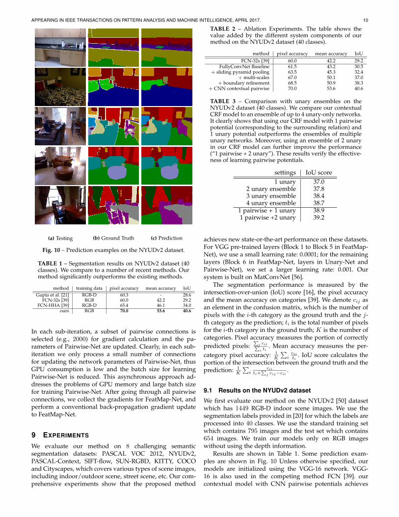
(a) Testing (b) Ground Truth (c) Prediction

Fig. 10 – Prediction examples on the NYUDv2 dataset.

TABLE 1 – Segmentation results on NYUDv2 dataset (40classes). We compare to a number of recent methods. Ourmethod significantly outperforms the existing methods.

method training data pixel accuracy mean accuracy IoUGupta et al. [21] RGB-D 60.3 - 28.6

FCN-32s [39] RGB 60.0 42.2 29.2FCN-HHA [39] RGB-D 65.4 46.1 34.0

ours RGB 70.0 53.6 40.6

In each sub-iteration, a subset of pairwise connections isselected (e.g., 2000) for gradient calculation and the pa-rameters of Pairwise-Net are updated. Clearly, in each sub-iteration we only process a small number of connectionsfor updating the network parameters of Pairwise-Net, thusGPU consumption is low and the batch size for learningPairwise-Net is reduced. This asynchronous approach ad-dresses the problems of GPU memory and large batch sizefor training Pairwise-Net. After going through all pairwiseconnections, we collect the gradients for FeatMap-Net, andperform a conventional back-propagation gradient updateto FeatMap-Net.

9 EXPERIMENTS

We evaluate our method on 8 challenging semanticsegmentation datasets: PASCAL VOC 2012, NYUDv2,PASCAL-Context, SIFT-flow, SUN-RGBD, KITTY, COCOand Cityscapes, which covers various types of scene images,including indoor/outdoor scene, street scene, etc. Our com-prehensive experiments show that the proposed method

TABLE 2 – Ablation Experiments. The table shows thevalue added by the different system components of ourmethod on the NYUDv2 dataset (40 classes).

method pixel accuracy mean accuracy IoUFCN-32s [39] 60.0 42.2 29.2

FullyConvNet Baseline 61.5 43.2 30.5+ sliding pyramid pooling 63.5 45.3 32.4

+ multi-scales 67.0 50.1 37.0+ boundary refinement 68.5 50.9 38.3

+ CNN contextual pairwise 70.0 53.6 40.6

TABLE 3 – Comparison with unary ensembles on theNYUDv2 dataset (40 classes). We compare our contextualCRF model to an ensemble of up to 4 unary-only networks.It clearly shows that using our CRF model with 1 pairwisepotential (corresponding to the surrounding relation) and1 unary potential outperforms the ensembles of multipleunary networks. Moreover, using an ensemble of 2 unaryin our CRF model can further improve the performance(“1 pairwise + 2 unary”). These results verify the effective-ness of learning pairwise potentials.

settings IoU score1 unary 37.0

2 unary ensemble 37.83 unary ensemble 38.44 unary ensemble 38.7

1 pairwise + 1 unary 38.91 pairwise +2 unary 39.2

achieves new state-or-the-art performance on these datasets.For VGG pre-trained layers (Block 1 to Block 5 in FeatMap-Net), we use a small learning rate: 0.0001; for the remaininglayers (Block 6 in FeatMap-Net, layers in Unary-Net andPairwise-Net), we set a larger learning rate: 0.001. Oursystem is built on MatConvNet [56].

The segmentation performance is measured by theintersection-over-union (IoU) score [16], the pixel accuracyand the mean accuracy on categories [39]. We denote cij asan element in the confusion matrix, which is the number ofpixels with the i-th category as the ground truth and the j-th category as the prediction; ti is the total number of pixelsfor the i-th category in the ground truth; K is the number ofcategories. Pixel accuracy measures the portion of correctlypredicted pixels:

∑i cii∑i ti

. Mean accuracy measures the per-category pixel accuracy: 1

K

∑iciiti

. IoU score calculates theportion of the intersection between the ground truth and theprediction: 1

K

∑i

ciiti+

∑j cij−cii .

9.1 Results on the NYUDv2 dataset

We first evaluate our method on the NYUDv2 [50] datasetwhich has 1449 RGB-D indoor scene images. We use thesegmentation labels provided in [20] for which the labels areprocessed into 40 classes. We use the standard training setwhich contains 795 images and the test set which contains654 images. We train our models only on RGB imageswithout using the depth information.

Results are shown in Table 1. Some prediction exam-ples are shown in Fig. 10 Unless otherwise specified, ourmodels are initialized using the VGG-16 network. VGG-16 is also used in the competing method FCN [39]. ourcontextual model with CNN pairwise potentials achieves


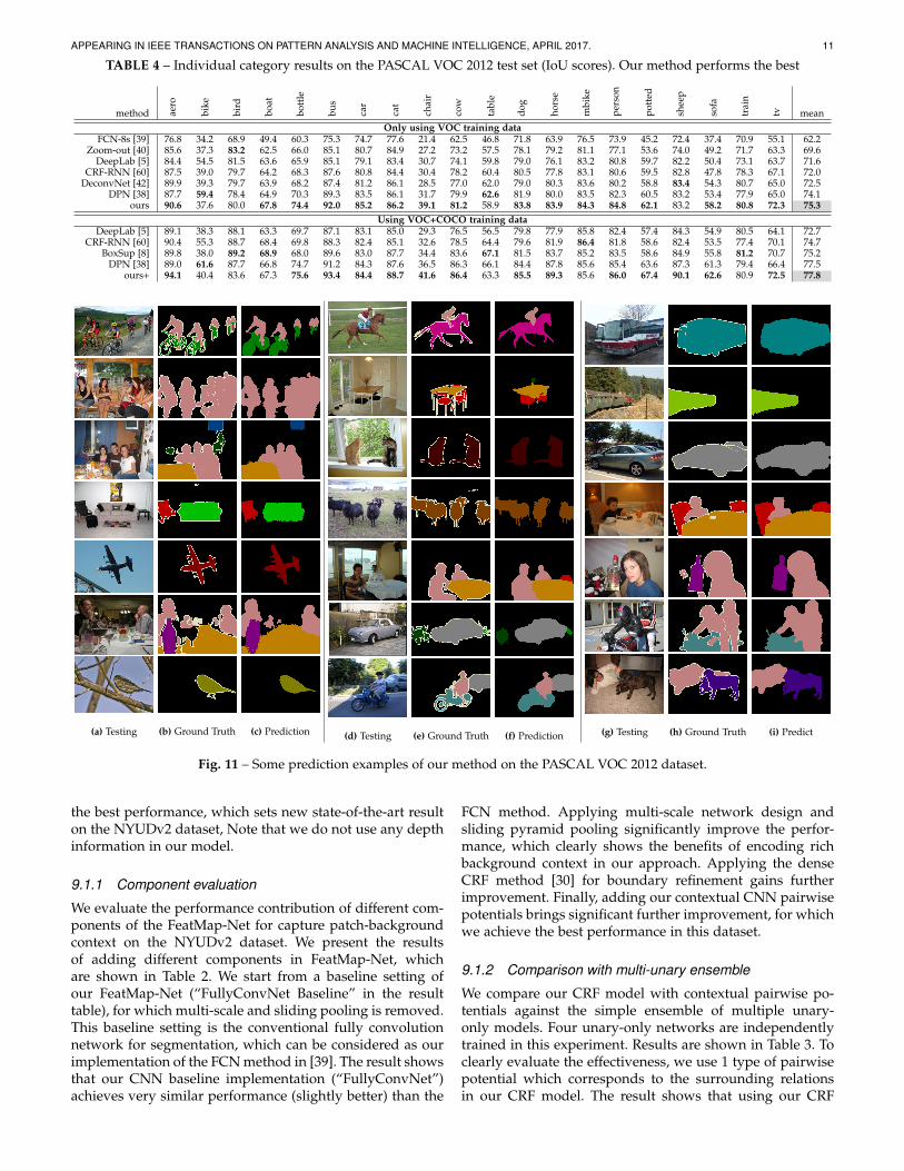
TABLE 4 – Individual category results on the PASCAL VOC 2012 test set (IoU scores). Our method performs the best

method aero

bike

bird

boat

bott

le

bus

car

cat

chai

r

cow

tabl

e

dog

hors

e

mbi

ke

pers

on

pott

ed

shee

p

sofa

trai

n

tv meanOnly using VOC training data

FCN-8s [39] 76.8 34.2 68.9 49.4 60.3 75.3 74.7 77.6 21.4 62.5 46.8 71.8 63.9 76.5 73.9 45.2 72.4 37.4 70.9 55.1 62.2Zoom-out [40] 85.6 37.3 83.2 62.5 66.0 85.1 80.7 84.9 27.2 73.2 57.5 78.1 79.2 81.1 77.1 53.6 74.0 49.2 71.7 63.3 69.6

DeepLab [5] 84.4 54.5 81.5 63.6 65.9 85.1 79.1 83.4 30.7 74.1 59.8 79.0 76.1 83.2 80.8 59.7 82.2 50.4 73.1 63.7 71.6CRF-RNN [60] 87.5 39.0 79.7 64.2 68.3 87.6 80.8 84.4 30.4 78.2 60.4 80.5 77.8 83.1 80.6 59.5 82.8 47.8 78.3 67.1 72.0

DeconvNet [42] 89.9 39.3 79.7 63.9 68.2 87.4 81.2 86.1 28.5 77.0 62.0 79.0 80.3 83.6 80.2 58.8 83.4 54.3 80.7 65.0 72.5DPN [38] 87.7 59.4 78.4 64.9 70.3 89.3 83.5 86.1 31.7 79.9 62.6 81.9 80.0 83.5 82.3 60.5 83.2 53.4 77.9 65.0 74.1

ours 90.6 37.6 80.0 67.8 74.4 92.0 85.2 86.2 39.1 81.2 58.9 83.8 83.9 84.3 84.8 62.1 83.2 58.2 80.8 72.3 75.3Using VOC+COCO training data

DeepLab [5] 89.1 38.3 88.1 63.3 69.7 87.1 83.1 85.0 29.3 76.5 56.5 79.8 77.9 85.8 82.4 57.4 84.3 54.9 80.5 64.1 72.7CRF-RNN [60] 90.4 55.3 88.7 68.4 69.8 88.3 82.4 85.1 32.6 78.5 64.4 79.6 81.9 86.4 81.8 58.6 82.4 53.5 77.4 70.1 74.7

BoxSup [8] 89.8 38.0 89.2 68.9 68.0 89.6 83.0 87.7 34.4 83.6 67.1 81.5 83.7 85.2 83.5 58.6 84.9 55.8 81.2 70.7 75.2DPN [38] 89.0 61.6 87.7 66.8 74.7 91.2 84.3 87.6 36.5 86.3 66.1 84.4 87.8 85.6 85.4 63.6 87.3 61.3 79.4 66.4 77.5

ours+ 94.1 40.4 83.6 67.3 75.6 93.4 84.4 88.7 41.6 86.4 63.3 85.5 89.3 85.6 86.0 67.4 90.1 62.6 80.9 72.5 77.8

(a) Testing (b) Ground Truth (c) Prediction (d) Testing (e) Ground Truth (f) Prediction (g) Testing (h) Ground Truth (i) Predict

Fig. 11 – Some prediction examples of our method on the PASCAL VOC 2012 dataset.

the best performance, which sets new state-of-the-art resulton the NYUDv2 dataset, Note that we do not use any depthinformation in our model.

9.1.1 Component evaluation

We evaluate the performance contribution of different com-ponents of the FeatMap-Net for capture patch-backgroundcontext on the NYUDv2 dataset. We present the resultsof adding different components in FeatMap-Net, whichare shown in Table 2. We start from a baseline setting ofour FeatMap-Net (“FullyConvNet Baseline” in the resulttable), for which multi-scale and sliding pooling is removed.This baseline setting is the conventional fully convolutionnetwork for segmentation, which can be considered as ourimplementation of the FCN method in [39]. The result showsthat our CNN baseline implementation (“FullyConvNet”)achieves very similar performance (slightly better) than the

FCN method. Applying multi-scale network design andsliding pyramid pooling significantly improve the perfor-mance, which clearly shows the benefits of encoding richbackground context in our approach. Applying the denseCRF method [30] for boundary refinement gains furtherimprovement. Finally, adding our contextual CNN pairwisepotentials brings significant further improvement, for whichwe achieve the best performance in this dataset.

9.1.2 Comparison with multi-unary ensemble

We compare our CRF model with contextual pairwise po-tentials against the simple ensemble of multiple unary-only models. Four unary-only networks are independentlytrained in this experiment. Results are shown in Table 3. Toclearly evaluate the effectiveness, we use 1 type of pairwisepotential which corresponds to the surrounding relationsin our CRF model. The result shows that using our CRF


model with 1 pairwise potential and 1 unary potential (“1pairwise + 1 unary”) outperforms the ensembles of multipleunary networks, which verifies the effectiveness of learningpairwise potentials. Moreover, using extra unary networks,i.e., an ensemble of 2 unary networks, in our CRF model canfurther improve the performance, as shown by the entry “1pairwise + 2 unary” in the result table. It indicates that ourpairwise potential is able to capture different informationand complementary to the multi-unary ensemble.

9.2 Results on the PASCAL VOC 2012 dataset

PASCAL VOC 2012 [16] is a well-known segmentation eval-uation dataset which consists of 20 object categories and onebackground category. This dataset is split into a training set,a validation set and a test set, which respectively contain1464, 1449 and 1456 images. Following a conventionalsetting in [5], [24], the training set is augmented by extraannotated VOC images provided in [22], which results in10582 training images. We verify our performance on thePASCAL VOC 2012 test set. We compare with a numberof recent methods with competitive performance. Since theground truth labels are not available for the test set, weevaluate our method through the VOC evaluation server.

The IoU scores are shown in the last column of Table4. Prediction examples of our method are shown in Fig.11. We first train our model only using the VOC images.We achieve an IoU score of 75.3, which is the best resultamongst methods that only use the VOC training data.1

To improve the performance, following the setting inrecent work [5], [8], we train our model with the extra im-ages from the COCO dataset [34]. With these extra trainingimages, we achieve an IoU score of 77.2.

As described in Sec. 6, our deep structured model gen-erates low-resolution coarse prediction, which is 1/16 ofthe input image size. To obtain the final high-resolutionprediction we apply a simple yet effective approach: we firstperform bilinear upsampling of the coarse score map andthen apply the boundary refinement post-processing [30].To improving this simple approach, we exploit the featuremaps from middle layers to refine the coarse prediction andproduce high-resolution prediction, which is similar to themethods in [5], [23], [39]. With this improved refinementapproach, we finally achieve an IoU score of 77.8, which isbest reported result on this challenging dataset. 2

The feature maps from the middle layers encodelower level visual information (from edge patterns to tex-ture/object part patterns) and have higher resolution thanthe final output, thus it is expected that learning extra layerson these feature maps helps to predict details in the objectboundaries. Specifically, we add refinement layers on topof the feature maps from the first 5 max-pooling layersand the score map of the coarse prediction (output by ourdeep structured model). Details are shown in Fig. 12. Theserefinement layers play a role of refining the coarse predic-tion by exploring middle layer features, which increase theresolution of the prediction from 1/16 (coarse prediction)

1. The result link at the VOC evaluation server: http://host.robots.ox.ac.uk:8080/anonymous/KEFFM4.html

2. The result link at the VOC evaluation server: http://host.robots.ox.ac.uk:8080/anonymous/MVTNTX.html

1/1 size

Input Image

1/2 size 1/4 size

1/16 size

Feature maps from top 5 max-pooling layers

Input score map (coarse prediction)

Apply 2 Conv layers for each feature map

upsample and concatenate

1/2 size3 Conv layers

1/2 size

Refined score map

Fig. 12 – The illustration of exploiting the feature mapsfrom middle layers to refine the low-resolution (1/16 ofthe input image) coarse prediction. The refined predictionhas a resolution of 1/2 of the input image.

TABLE 5 – Segmentation results on the Cityscapes test set.our method achieves the best performance.

Method IoU scoreFCN-8s [39] 65.3

DPN [38] 66.8Dilation10 [58] 67.1

DeepLab-CRF [5] 63.1ours 71.6

to 1/2 of the input image. With this improved prediction,we perform boundary refinement using [30] to generate thefinal prediction.

The results for each category are shown in Table 4. Weoutperform comparing methods in most categories. For onlyusing the VOC training set, our method outperforms the sec-ond best method, DPN [38], on 18 categories out of 20. Forusing VOC+COCO training set, our method outperformsDPN [38] on 15 categories out of 20.

9.3 Results on the Cityscapes datasetThe large scale outdoor image dataset Cityscapes [7] con-tains high-resolution street scene images from 50 differentcities. This dataset provides pixel-level semantic segmen-tation labels of 5000 images for 25 classes including road,car, pedestrian, bicycle, sky etc. The provided “trainval” sethas 3475 image. We use the training set (2975 images) fortraining. The ground truth of the test set is not available, andwe evaluate our method through their evaluation server.We follow the provided protocol for dataset evaluation: 19classes are valid for evaluation, and the remaining 6 classesare not considered in evaluation.

Results are shown in Table 5. As similar to the setting forthe PASCAL VOC dataset, we train a refinement networkwhich is described in Fig. 12 to obtain high resolution pre-diction. Here we set the output resolution in the refinementnetwork as 1/4 of the input image size. The result clearlyshows that our method outperforms other competing meth-ods. Prediction examples on the validation set are shown inFig. 13.

9.4 Results on the PASCAL-Context datasetThe PASCAL-Context [41] dataset provides the segmenta-tion labels of the whole scene (including the “stuff” labels)for the PASCAL VOC images. We use the segmentationlabels which contain 60 classes (59 classes plus the “

http://host.robots.ox.ac.uk:8080/anonymous/KEFFM4.html

http://host.robots.ox.ac.uk:8080/anonymous/KEFFM4.html

http://host.robots.ox.ac.uk:8080/anonymous/MVTNTX.html

http://host.robots.ox.ac.uk:8080/anonymous/MVTNTX.html


(a) Testing (b) Ground Truth (c) Prediction (d) Testing (e) Ground Truth (f) Prediction

Fig. 13 – Prediction examples of our method on Cityscapes dataset.

TABLE 6 – Segmentation results on PASCAL-Contextdataset (60 classes). Our method performs the best.

method pixel accuracy mean accuracy IoUO2P [4] - - 18.1

CFM [9] - - 34.4FCN-8s [39] 65.9 46.5 35.1BoxSup [8] - - 40.5

ours 71.5 53.9 43.3

TABLE 7 – Segmentation results on SUN-RGBD dataset(37 classes). We compare to a number of recent methods.Our method significantly outperforms the existing meth-ods.

method training data pixel accuracy mean accuracy IoULiu et al. [35] RGB-D − 10.0 −Ren et al. [47] RGB-D − 36.3 −

Kendall et al. [28] RGB 71.2 45.9 30.7ours RGB 78.4 53.4 42.3

background” class ) for evaluation. We use the providedtraining/test splits. The training set contains 4998 imagesand the test set contains 5105 images.

Results are shown in Table 6. Prediction examples areshown in Fig. 14 Our method significantly outperform thecompeting methods. To our knowledge, ours is the bestreported result on this dataset.

9.5 Results on the SUN-RGBD datasetSUN-RGBD [52] is a segmentation dataset contains around10, 000 indoor images and provides pixel labeling masks of37 classes, which is an extension of the NYUD dataset [50].Results are shown in Table 7. Our method outperform theexisting methods by a large margin, even though we doesnot make use of the depth information for training.

9.6 Results on the COCO datasetThe COCO dataset [34] contains more than 1 million imagesand provide segmentation labels for 80 classes. Since the test

TABLE 8 – Segmentation results on COCO dataset (80classes). Our method significantly outperforms the fullyconvolution network (“FullyConvNet”).

method pixel accuracy mean accuracy IoUFullyConvNet 84.2 56.9 37.2

FullyConvNet + refine 86.7 55.0 41.3ours 88.3 58.7 46.8

TABLE 9 – Segmentation results on SIFT-flow dataset (33classes). Our method performs the best.

method pixel accuracy mean accuracy IoULiu et al. [35] 76.7 - -

Tighe et al. [54] 75.6 41.1 -Tighe et al. (MRF) [54] 78.6 39.2 -

Farabet et al. (balance) [17] 72.3 50.8 -Farabet et al. [17] 78.5 29.6 -

Pinheiro et al. [45] 77.7 29.8 -FCN-16s [39] 85.2 51.7 39.5

ours 88.1 53.4 44.9

set is not available, we generate 2599 images for testing andthe remaining images are for training. We select the test im-ages on a class balance basis which ensures every categoryat lease appears in 50 images. Labeling regions which aresmaller than 200 pixels are treated as “void” which are notconsidered in training and evaluation. Results are shownin Table 8. We compared to two baseline methods whichare based on conventional fully convolution networks. Thedetails of these baseline methods are the same as that for theCityscapes dataset (see Sec. 9.3). The results shows that ourmethod significantly outperforms the baselines.

9.7 Results on the SIFT-flow datasetWe further evaluate our method on the SIFT-flow dataset.This dataset contains 2688 images and provides the seg-mentation labels for 33 classes. We use the standard split fortraining and evaluation. The training set has 2488 imagesand the test set has 200 images. Since the images are in


TABLE 10 – Segmentation results on KITTI dataset (10classes). We compare to a number of recent methods. Ourmethod significantly outperforms the existing methods.

method pixel accuracy mean accuracy IoUCadena et al. [3] 84.1 52.4 −Zhang et al. [59] 89.3 65.4 −

ours 93.3 74.5 68.5ours+ 94.3 75.9 70.3

small sizes, we upscale the image by a factor of 2 fortraining. Results are shown in Table 9. We achieve the bestperformance on this dataset.

9.8 Results on the KITTI dataset

We perform further evaluation on the KITTI dataset [18] forroad image segmentation. Zhang at el. [59] provide semanticsegmentation labels of 10 classes for 252 images, in which140 images are for training and the remaining 112 are fortesting. We follow the provided training and testing splitsfor evaluation and report the results in Table 10. Clearly,our method performs the best. To further improve theperformance, we perform pre-training on COCO images, forwhich the result is denoted by “ours+” in the result table.

10 CONCLUSIONS

We have proposed a method which combines CNNs andCRFs to exploit complex contextual information for semanticimage segmentation. Basically, we formulate CNN basedpairwise potentials for modeling semantic relations betweenimage regions. We have performed comprehensive exper-iments on 8 challenging segmentation datasets and weachieve state-of-the-art performance on all evaluated datasetincluding the PASCAL VOC 2012 dataset. The proposedmethod is potentially widely applicable to other tasks.

ACKNOWLEDGMENTS

This research was supported by Australian ResearchCouncil through the ARC Centre for Robotic Vision(CE140100016). C. Shen’s participation was in part sup-ported by an ARC Future Fellowship (FT120100969). I.Reid’s participation was in part supported by an ARCLaureate Fellowship (FL130100102).

REFERENCES

[1] Y. Bengio. Practical recommendations for gradient-based trainingof deep architectures. CoRR, abs/1206.5533, 2012.

[2] J. Besag. Efficiency of pseudolikelihood estimation for simpleGaussian fields. Biometrika, 1977.

[3] C. Cadena and J. Kosecka. Semantic segmentation with heteroge-neous sensor coverages. In IEEE International Conference on Roboticsand Automation (ICRA), 2014.

[4] J. Carreira, R. Caseiro, J. Batista, and C. Sminchisescu. Semanticsegmentation with second-order pooling. In Proc. Eur. Conf. Comp.Vis., 2012.

[5] L. Chen, G. Papandreou, I. Kokkinos, K. Murphy, and A. L. Yuille.Semantic image segmentation with deep convolutional nets andfully connected CRFs. In Proc. Int. Conf. Learning Representations,2015.

[6] L.-C. Chen, A. G. Schwing, A. L. Yuille, and R. Urtasun. Learningdeep structured models. In Proc. Int. Conf. Machine Learn., 2015.

[7] M. Cordts, M. Omran, S. Ramos, T. Rehfeld, M. Enzweiler, R. Be-nenson, U. Franke, S. Roth, and B. Schiele. The cityscapes datasetfor semantic urban scene understanding. In CVPR, 2016.

[8] J. Dai, K. He, and J. Sun. BoxSup: Exploiting bounding boxes tosupervise convolutional networks for semantic segmentation. InProc. Int. Conf. Comp. Vis., 2015.

[9] J. Dai, K. He, and J. Sun. Convolutional feature masking forjoint object and stuff segmentation. In Proc. IEEE Conf. Comp. Vis.Pattern Recogn., 2015.

[10] J. Dean, G. Corrado, R. Monga, K. Chen, M. Devin, M. Mao, A. Se-nior, P. Tucker, K. Yang, Q. V. Le, et al. Large scale distributed deepnetworks. In Advances in Neural Information Processing Systems,2012.

[11] C. Doersch, A. Gupta, and A. A. Efros. Context as supervisorysignal: Discovering objects with predictable context. In Proc.European Conf. Computer Vision, 2014.

[12] C. Dong, C. C. Loy, K. He, and X. Tang. Learning a deepconvolutional network for image super-resolution. In Proc. Eur.Conf. Comp. Vis., 2014.

[13] D. Eigen and R. Fergus. Predicting depth, surface normals andsemantic labels with a common multi-scale convolutional architec-ture. In Proceedings of the IEEE International Conference on ComputerVision, 2015.

[14] D. Eigen, D. Krishnan, and R. Fergus. Restoring an image takenthrough a window covered with dirt or rain. In Proc. Int. Conf.Comp. Vis., 2013.

[15] D. Eigen, C. Puhrsch, and R. Fergus. Depth map prediction froma single image using a multi-scale deep network. In Proc. Adv.Neural Info. Process. Syst., 2014.

[16] M. Everingham, L. Van Gool, C. K. Williams, J. Winn, and A. Zis-serman. The pascal visual object classes (voc) challenge. In Proc.Int. J. Comp. Vis., 2010.

[17] C. Farabet, C. Couprie, L. Najman, and Y. LeCun. Learninghierarchical features for scene labeling. IEEE T. Pattern Analysis& Machine Intelligence, 2013.

[18] A. Geiger, P. Lenz, and R. Urtasun. Are we ready for autonomousdriving? the kitti vision benchmark suite. In Proc. IEEE Conf. Comp.Vis. Pattern Recogn., 2012.

[19] R. B. Girshick, J. Donahue, T. Darrell, and J. Malik. Rich feature hi-erarchies for accurate object detection and semantic segmentation.In Proc. IEEE Conf. Comp. Vis. Pattern Recogn., 2014.

[20] S. Gupta, P. Arbelaez, and J. Malik. Perceptual organization andrecognition of indoor scenes from rgb-d images. In Proc. IEEEConf. Comp. Vis. Pattern Recogn., 2013.

[21] S. Gupta, R. Girshick, P. Arbelaez, and J. Malik. Learning richfeatures from rgb-d images for object detection and segmentation.In Proc. Eur. Conf. Comp. Vis., 2014.

[22] B. Hariharan, P. Arbelaez, L. D. Bourdev, S. Maji, and J. Malik.Semantic contours from inverse detectors. In Proc. Int. Conf. Comp.Vis., 2011.

[23] B. Hariharan, P. Arbelaez, R. Girshick, and J. Malik. Hypercolumnsfor object segmentation and fine-grained localization. In Proc. IEEEConf. Comp. Vis. Pattern Recogn., 2014.

[24] B. Hariharan, P. Arbelaez, R. Girshick, and J. Malik. Simultaneousdetection and segmentation. In Proc. European Conf. ComputerVision, 2014.

[25] D. Heesch and M. Petrou. Markov random fields with asymmet-ric interactions for modelling spatial context in structured scenelabelling. Journal of Signal Processing Systems, 2010.

[26] G. Heitz and D. Koller. Learning spatial context: Using stuff tofind things. In Proc. European Conf. Computer Vision, 2008.

[27] J. Jancsary, S. Nowozin, T. Sharp, and C. Rother. Regressiontree fieldsan efficient, non-parametric approach to image labelingproblems. In Proc. IEEE Conf. Comp. Vis. Pattern Recogn., 2012.

[28] A. Kendall, V. Badrinarayanan, and R. Cipolla. Bayesian segnet:Model uncertainty in deep convolutional encoder-decoder archi-tectures for scene understanding. CoRR, abs/1511.02680, 2015.

[29] A. Kolesnikov, M. Guillaumin, V. Ferrari, and C. H. Lampert.Closed-form training of conditional random fields for large scaleimage segmentation. In Proc. Eur. Conf. Comp. Vis., 2014.

[30] P. Krahenbuhl and V. Koltun. Efficient inference in fully connectedCRFs with Gaussian edge potentials. In Proc. Adv. Neural Info.Process. Syst., 2012.

[31] S. Lazebnik, C. Schmid, and J. Ponce. Beyond bags of features: Spa-tial pyramid matching for recognizing natural scene categories. InProc. IEEE Conf. Comp. Vis. Pattern Recogn., 2006.

[32] M. Li, T. Zhang, Y. Chen, and A. J. Smola. Efficient mini-batchtraining for stochastic optimization. In Proceedings of the 20thACM SIGKDD international conference on Knowledge discovery anddata mining, 2014.


(a) Testing (b) Ground Truth (c) Prediction

Fig. 14 – Prediction examples on the PASCAL-Context dataset.

[33] G. Lin, C. Shen, A. van den Hengel, and I. Reid. Efficient piecewisetraining of deep structured models for semantic segmentation. InProc. IEEE Conf. Comp. Vis. Pattern Recogn., 2016.

[34] T.-Y. Lin, M. Maire, S. Belongie, J. Hays, P. Perona, D. Ramanan,P. Dollar, and C. L. Zitnick. Microsoft COCO: Common objects incontext. In Proc. Eur. Conf. Comp. Vis., 2014.

[35] C. Liu, J. Yuen, and A. Torralba. Sift flow: Dense correspondenceacross scenes and its applications. IEEE T. Pattern Analysis &Machine Intelligence, 2011.

[36] F. Liu, C. Shen, and G. Lin. Deep convolutional neural fields fordepth estimation from a single image. In Proc. IEEE Conf. Comp.Vis. Pattern Recogn., 2015.

[37] F. Liu, C. Shen, G. Lin, and I. Reid. Learning depth from singlemonocular images using deep convolutional neural fields, 2015.http://arxiv.org/abs/1502.07411.

[38] Z. Liu, X. Li, P. Luo, C. C. Loy, and X. Tang. Semantic imagesegmentation via deep parsing network. In Proc. Int. Conf. Comp.Vis., 2015.

[39] J. Long, E. Shelhamer, and T. Darrell. Fully convolutional networksfor semantic segmentation. In Proc. IEEE Conf. Comp. Vis. PatternRecogn., 2015.

[40] M. Mostajabi, P. Yadollahpour, and G. Shakhnarovich. Feedfor-ward semantic segmentation with zoom-out features. In Proc. IEEEConf. Comp. Vis. Pattern Recogn., 2015.

[41] R. Mottaghi, X. Chen, X. Liu, N.-G. Cho, S.-W. Lee, S. Fidler,R. Urtasun, et al. The role of context for object detection and

semantic segmentation in the wild. In Proc. IEEE Conf. Comp. Vis.Pattern Recogn., 2014.

[42] H. Noh, S. Hong, and B. Han. Learning deconvolution networkfor semantic segmentation. In Proc. Int. Conf. Comp. Vis., 2015.

[43] S. Nowozin and C. Lampert. Structured learning and predictionin computer vision. Found. Trends. Comput. Graph. Vis., 2011.

[44] S. Nowozin, C. Rother, S. Bagon, T. Sharp, B. Yao, and P. Kohli.Decision tree fields. In Proc. Int. Conf. Comp. Vis., 2011.

[45] P. H. Pinheiro and R. Collobert. Recurrent convolutional neuralnetworks for scene parsing. In Proc. Int. Conf. Machine Learn., 2014.

[46] A. Rabinovich, A. Vedaldi, C. Galleguillos, E. Wiewiora, andS. Belongie. Objects in context. In Proc. Int. Conf. Comp. Vis., 2007.

[47] X. Ren, L. Bo, and D. Fox. Rgb-(d) scene labeling: Features andalgorithms. In Proc. IEEE Conf. Comp. Vis. Pattern Recogn., 2012.

[48] A. G. Schwing and R. Urtasun. Fully connected deep structurednetworks, 2015. http://arxiv.org/abs/1503.02351.

[49] J. Shotton, J. Winn, C. Rother, and A. Criminisi. Textonboost forimage understanding: Multi-class object recognition and segmen-tation by jointly modeling texture, layout, and context. Interna-tional Journal of Computer Vision, 81(1):2–23, 2009.

[50] N. Silberman, D. Hoiem, P. Kohli, and R. Fergus. Indoor segmen-tation and support inference from rgbd images. In Proc. Eur. Conf.Comp. Vis., 2012.

[51] K. Simonyan and A. Zisserman. Very deep convolutional net-works for large-scale image recognition. In Proc. Int. Conf. LearningRepresentations, 2015.

http://arxiv.org/abs/1502.07411

http://arxiv.org/abs/1503.02351


[52] S. Song, S. P. Lichtenberg, and J. Xiao. Sun rgb-d: A rgb-d sceneunderstanding benchmark suite. In Proc. IEEE Conf. Comp. Vis.Pattern Recogn., 2015.

[53] C. A. Sutton and A. McCallum. Piecewise training for undirectedmodels. In Proc. Conf. Uncertainty Artificial Intelli, 2005.

[54] J. Tighe and S. Lazebnik. Finding things: Image parsing withregions and per-exemplar detectors. In Proc. IEEE Conf. Comp.Vis. Pattern Recogn., 2013.

[55] J. Tompson, A. Jain, Y. LeCun, and C. Bregler. Joint training ofa convolutional network and a graphical model for human poseestimation. In Proc. Adv. Neural Info. Process. Syst., 2014.

[56] A. Vedaldi and K. Lenc. MatConvNet – convolutional neuralnetworks for matlab, 2014.

[57] J. Winn and J. Shotton. The layout consistent random field forrecognizing and segmenting partially occluded objects. In Proc.IEEE Conf. Comp. Vis. Pattern Recogn., 2006.

[58] F. Yu and V. Koltun. Multi-scale context aggregation by dilatedconvolutions. CoRR, 2015.

[59] R. Zhang, S. Candra, K. Vetter, and A. Zakhor. Sensor fusionfor semantic segmentation of urban scenes. In IEEE InternationalConference on Robotics and Automation (ICRA), 2015.

[60] S. Zheng, S. Jayasumana, B. Romera-Paredes, V. Vineet, Z. Su,D. Du, C. Huang, and P. Torr. Conditional random fields asrecurrent neural networks. In Proc. Int. Conf. Comp. Vis., 2015.

Documents

1 Exploring Context with Deep Structured models for ... Exploring Context with Deep Structured models for Semantic Segmentation Guosheng Lin, Chunhua Shen, Anton van den Hengel, Ian