Embed Size (px)
Citation preview
1
EDUCATION AND CIVIC OUTCOMES IN ITALY
Giorgio Di Pietro* and Marcos Delprato University of Westminster Westminster Business School 35 Marylebone Road NW1 5LS London
Abstract
This paper examines the effect of education on civic outcomes in Italy. The analysis uses standard regression techniques such as OLS and ordered probit as well as IV and two-stage ordered probit methods in an attempt to account for the possibility that education is endogenous. In line with previous studies, our results show that the omission of unobserved factors makes OLS and ordered probit estimates on education to be biased. However, we find that the direction of this bias varies across different measures of civic outcomes. This result reconciles findings from previous studies (see, Dee, 2004; Milligan et al., 2004 and Gibson, 2001) showing mixed results about the causal effect of education on civic outcomes.
JEL Classification: I20, H80
*Corresponding author- email: [email protected] Tel: +44(0)2079115000 ext 3350- Fax: +44(0)2079115839 We are thankful to Thomas Dee, Enrico Moretti and seminar participants in the University of Girona for helpful comments on an earlier version of the paper. However, we are solely responsible for this paper’s contents.

2
1. Introduction
A vast number of studies in the political science and economic literature have analysed
the relationship between education and civic outcomes (for an extensive literature review,
see Campbell, 2006). However, one of the main problems in the estimation of this
relationship lies in the potential endogeneity bias associated with education. It is quite
possible that there are unobserved individual and family characteristics which
simultaneously affect education and civic outcomes. Suppose that some parents
encourage their children to place great value on education. If these same parents teach
their children about the importance of being civically responsible, then the empirical
association between education and civic outcomes would be spurious. This implies that if
a method designed to deal with “selection on unobservables” is not employed, education
will pick up the effect of omitted variables on civic outcomes.
Although several empirical studies have examined the impact of education on civic
outcomes accounting for the bias associated with the endogeneity of education, results
appear to be mixed. On the one hand, Gibson (2001) finds that the positive effect of
schooling on the probability of doing volunteer work is reversed once one controls for the
omitted-variables bias. On the other hand, Dee (2004) shows that increases in educational
attainment have large and statistically significant effects on voter participation and
support for free speech in the US and this result holds even when an instrumental variable
(IV) strategy is used in an attempt to address the problem of the endogeneity of education.
This finding is also consistent with Milligan et al. (2004) who, using a similar

3
methodology, find a positive relationship between education and voting behavior in the
US. Additionally, both Dee (2004) and Milligan et al. (2004) conclude that the omission
of unobserved factors makes OLS estimates on education to be biased downward relative
to the corresponding IV estimates.
In this paper, we attempt to reconcile these mixed results by examining the causal effect
of education on five different measures of civic outcomes. Our intuition is that, as civic
outcomes can be proxied by a vast array of measures, it is quite possible that those
unobservables that make an individual develop a taste for education may have a different
impact across these measures. For instance, consider individuals possessing unobserved
qualities such as “determination” and “drive”. On the one hand, these characteristics are
clearly correlated with educational attainment. On the other hand, however, their effect
on voter turnout may be opposite to that on doing volunteer work. Possessing more
“determination” and “drive” may discourage individuals from participating in political
elections as they are mindful that their vote has a minuscule probability of being
determinant, but at the same time it may make individuals more conscientious about their
responsibility in helping less advantaged people.
In addition to using several measures of civic outcomes, this paper extends previous
research in other two main aspects. First, in an attempt to account for the possibility that
civic outcomes are correlated with unobserved factors that also influence educational
attainment, we apply both standard IV and two-stage ordered probit estimation
techniques. Second, our attention is focused on Italy. Works on the US and the UK tend
4
dominate the empirical literature in this area and, whilst these studies are instructive, it
would be rather hazardous to make inference exclusively based on them.
The remainder of the paper is as follows. Section 2 reviews the literature on the effect of
education on civic and social engagement. Section 3 describes the data used in this study.
Section 4 presents and discusses the empirical results. Section 5 concludes.
2. Education and civic outcomes
There are several mechanisms whereby education may promote civic engagement. To
begin with, education in general can enhance cognitive proficiency and analytic ability.
This is important as, for instance, it allows more educated individuals to have a greater
capacity for absorbing and organising complex political information. Similarly, greater
cognitive proficiency and analytic ability may help people to deal with bureaucratic
procedures. For example, Wolfinger and Rosenstone (1980) find that in the US education
is likely to lead to a higher voter turnout because it facilitates voter registration.
Additionally, education may also help individuals to understand their own rights as well
as the civil rights of others.
However, a number of researchers have also formulated the hypothesis that the
relationship between education and civic outcomes could be negative. Higher educated
individuals may face a higher opportunity cost of time and this, in turn, may make them
spend less time and attention on civic activities. Although this consideration is likely to

5
be especially relevant for those civic activities that are particularly time-consuming (e.g.
volunteer work), Dee (2004) argues that it may also hold for voter participation. As
outlined in the introduction, higher educated individuals may be discouraged from
participating in political elections as they are aware that their vote has an infinitesimally
small probability of influencing actual policy.
A direct channel through which education is likely to impact on civic outcomes is
represented by civic courses. Although several studies show a positive relationship
between civics instruction and civic outcomes (Niemi and Junn, 1998; Torney-Purta,
2002), other researchers have questioned this finding. For instance, Langton and Jennings
(1968) conclude that classroom instruction in democratic education has virtually no
impact on political and civic outcomes. This result is consistent with that obtained by
Miller (1985) who, using longitudinal data, concludes that there little or no relationship
between civic education in secondary schools and the kind or amount of political
information of adults. Three main reasons have been offered to explain the
ineffectiveness of civic courses. First, they may provide students with information that is
mainly redundant. This occurs not only as some of the content of the civic courses is
covered by lectures in other disciplines, but also because students may obtain the same
information from other sources such as mass media and/or their parents. US students cite
TV news as the most important source of political information. Second, civics instruction
is supposed to be almost universal as it is received by students at a time when education
is compulsory. Thus if each student receives the same amount of instruction in civics,
then civics instruction will be unable to predict differences in civic engagement. The third

6
explanation may lie in poor quality teaching. There is the possibility that civics is not
taught using appropriate methods and/or is taught by individuals who have a lack of
interest in this subject. The crucial role of teachers in the development of civic attitudes is
highlighted by Ehman (1980) and Leming (1985).
Finally, several commentators argue that one of the reasons why schooling has a positive
impact on civic outcomes is because a class represents an environment which is
conducive to learning civic skills. Classroom activities include participation in debates
over political issues as well as participation in workshops where students learn to think
critically and to make decisions democratically. Additionally, extracurricular activities
may also be beneficial. Using data from the US National Education Longitudinal Study,
Smith (1999) finds that extracurricular activities in the eight, tenth and twelfth grades are
positively related to political participation two year after high school graduation.
Nevertheless, the hypothesis that participation in high school groups may have a
significant impact on subsequent political participation has been called into question by
Campbell (2006). He argues that both actions may be driven by unobserved
characteristics. More specifically, those unobservables which make an individual more
likely to join high school groups may also exert a positive influence on the probability
that he/she will participate in political elections.

7
3. Data
The main data used in this study come from the Survey of the Household Income and
Wealth (SHIW) carried out by the Central Bank of Italy. The 2004 wave of the SHIW
contains a special section that includes questions directly related to civic outcomes. This
section was only addressed to household heads born in uneven years.
In this study we consider five civic-related questions. The first one is about political
engagement as respondents were asked to indicate “how interested they are in politics”.
Answers to this question ranges from 1 to 4, which correspond to “very”, “fairly”, “not
very” and “not at all”, respectively. In the next three questions respondents were asked to
indicate the extent to which the following behaviors were justified: “not paying the ticket
on a public transport vehicle”, “keeping money you obtained by accident when it would
be possible to return it to the rightful owner” and “not leaving your name for the owner
of a car you accidentally scraped”. Responses to these questions are given on an ordered
scale from 1 for “never justifiable to 10 for “always justifiable”. Finally, in the last
question respondents were asked to “rate the importance of the problem of tax evasion in
relation to all the problems faced by the government”. The answer to this question is
coded on 1-5 scale, with 1 being “very serious”, 2 as “serious”, 3 as “the same as any
other”, 4 as “marginal” and 5 as “non-existent”. In an attempt to simplify the
interpretation of the empirical results, although the original scale of the responses to these
five questions has been kept, the order is reversed so high score indicates a higher sense
of civic duty.
8
While political engagement is a well-established proxy for civic outcomes, the rationale
for using the other indicators is that civic knowledge is expected to help citizens to learn
those skills needed to work with others towards goods that can only be created through
collective actions. Thus, every citizen has a moral responsibility to contribute to
sustaining the public institutions and processes on which the community is based, and
from which all its members benefit. Additionally, one should note that the use of civic
attitudes towards issues of public concern (e.g. corruption, tax evasion) finds increasing
support within the existing socio-economic literature. A recent example includes the
work by Algan and Cahuc (2006) in which they examine the determinants of civic
attitudes towards government benefits.
The survey reports only the highest educational attainment of the individual and not the
number of years he/she has spent at school. Following the approach employed in similar
studies (see, for instance, Vieira, 1999; Brunello and Miniaci, 1999) we compute a
continuous measure of education.1 Years of education are hence calculated by imputing
the number of years typically required to complete the highest level of educational
attainment reported by the individual. More precisely, the following procedure is used.
The number of statutory years required to obtain a primary school certificate and a lower
secondary school diploma are 5 and 8 years, respectively. As regards upper secondary
schools, the number of years depends on the type of school attended. While general
schools (licei) and technical schools (instituti tecnici e professionali) comprise a five-year
curriculum, teaching schools (istituti magistrali), which are specifically targeted to train
1 One of the main advantages of this approach is that it increases comparability across studies. On the other hand, in constructing a continuous measure of years of education we assume that returns to education are linear.

9
primary school teachers, are based on a four-year programme. The number of statutory
years required to complete university education varies according to the subject studied. It
ranges from 4 years for people who study humanities and social sciences to 6 years for
those who read medicine. Finally, most postgraduate courses tend to last one year in Italy.
In addition to schooling, a number of other explanatory factors are included in the model.
These are: gender, age and its square, marital status, employment status, household
income, number of children in the household, parental education and occupation, area of
residence and urban location.
In an attempt to narrow down the potential sources of variation that may lead to a bias in
the estimates of the effect of education on civic outcomes, we limit our analysis to men.
Several studies (see, for instance, Schlozman, et al. 1994) show that there are significant
gender differences in civic participation, with, for example, men more likely to be
engaged in politics than women. As this result is also likely to reflect differences in
unobservables, it is quite possible that the endogeneity bias of education in civic
outcomes equations may vary across gender. Summary statistics for the final sample are
presented in Table 1. There are 1,914 individuals in the sample2, with an average level of
9.5 years of education.
Insert Table 1 near here
2 3,798 household heads responded to the civic-related questions examined in this study. After focusing on men and dropping from the sample those individuals with missing relevant explanatory variables, we are left with 1,914 observations.

10
4. Empirical results
OLS and ordered probit
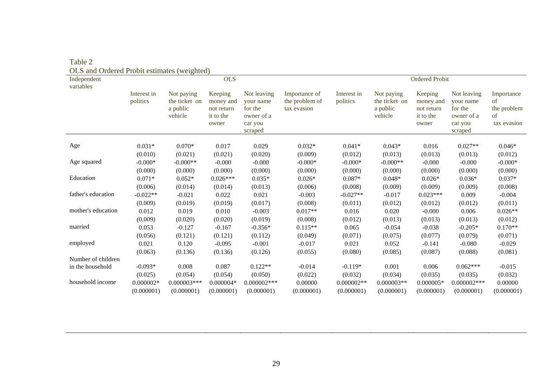
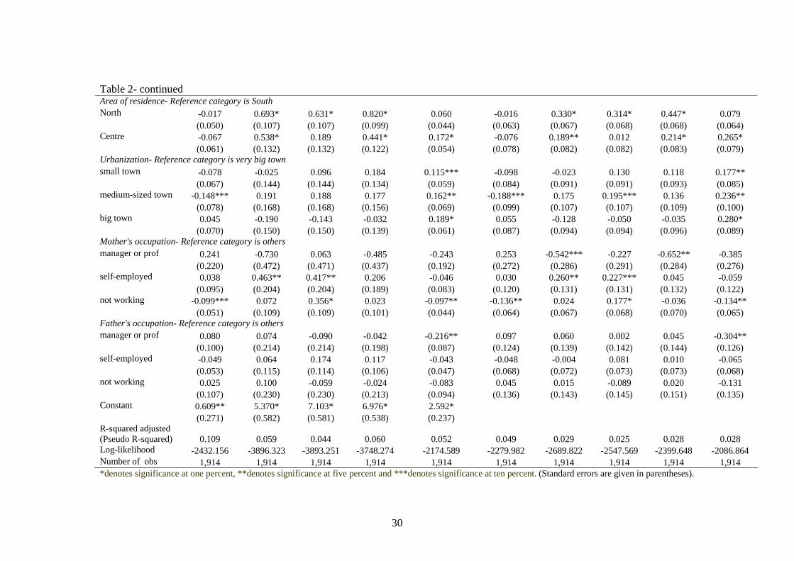
Table 2 presents the OLS and ordered probit estimates of the effect of education on our
five measures of civic outcomes. The coefficient on education is statistically significant
and has a positive sign in all the regressions shown in Table 2. This finding show that we
are able to reproduce the standard result in the literature- there is a positive and
statistically significant relationship in the data between education and civic outcomes.
Insert Table 2 near here
The results on the other explanatory variables are only briefly discussed here. The
coefficient on age is statistically significant in most OLS and ordered probit regressions.
Older individuals are likely to exhibit a higher concern for civic values relative to
younger individuals. This result is in line with that of Algan and Cahuc (2006) who,
using data on a number of OECD countries, find that the probability of considering it
unjustifiable to cheat on government benefits increases with age. Additionally, there is
some evidence that individuals living in the North tend to have a higher sense of civic
duty relative to those living in the South. The importance of geographical area as a
determinant of degree of ‘civicness’ in Italy has been emphasized by Ichino and Maggi
(2000). Employing data on a large Italian bank, they find that employees born in the
North are significantly less likely to shirk than those born in the South. There are also
11
significant effects associated with family income. Higher family income tends to lead to a
higher degree of ‘civicness’. The positive association between income and civic
outcomes is not an unusual result in the socio-economic literature. For instance,
Wolfinger and Rosenstone (1980) conclude that greater wealth and higher income
increase the likelihood of participating in elections.
There are two main potential sources of bias in the estimates reported in Table 2. First,
although we are aware that there is likely to be a measurement error in our indicators for
civic outcomes, our primary concern is on how this varies across educational levels.
Second, our estimates do not account for unobserved factors that affect both education
and civic outcomes. In what follows we attempt to tackle both these issues.
The issue of attitude-behaviour inconsistency
A first concern lies in the measurement error associated with our measures for civic
outcomes. As pointed out by Silver et al. (1986), it is possible that factors such as
pressure and guilt about civic responsibilities may make individuals overstate their sense
of civic duty. If misreporting is random across respondents, this affects the accuracy of
our estimates but it is not a source of bias. On the other hand, if misreporting is
systematically related to educational achievement, our estimates of the education
coefficient are biased.
12
Unfortunately, unlike other studies (see, for instance, Milligan et al., 2004) we are unable
to test whether misreporting is randomly distributed across educational levels. This is
because we cannot validate the answers to any of the civic questions included in the 2004
wave of the SHIW. However, in an attempt to provide some evidence on the scale of this
problem in Italy, we analyse data from another survey where, for at least one of our civic
measures (i.e. political engagement), there is the possibility to check whether civic
attitudes are connected with a specific action. This survey is the 2005 wave of the
“Multipurpose Survey. Aspects of Daily Life” (MSADL) carried out by the Italian
National Statistical Institute (ISTAT). It shares two important characteristics with the
SHIW: 1) in both surveys the final sample is representative of the Italian population; 2)
both surveys were conducted almost at the same time, i.e. the SHIW in 2004 and the
MSADL in 2005. Additionally, in order to make the results from the MSADL
comparable with those obtained from the SHIW, we select in the former only those male
individuals who are household heads and were born in uneven years in 2004.
From the 2005 wave of the MSADL we focus our attention on two questions on political
engagement. The first question asks individuals to indicate: “how often do they talk about
politics”. Answers to this question are on a six-point scale, as follows: “every day”,
“sometimes a week”, “once a week”, “sometimes a month (less than four)”, “sometimes a
year” and “never”. The second question asks the respondents to indicate whether they
“participated in the political election that took place in Italy in 2001”.3 Our strategy is to
3 Although self-reported measures of voting could be reasonably expected to contain some errors, several studies argue that they can still provide meaningful indicators for research purposes. For instance, Sigelman (1982, p. 53) concludes that “it seems safe to say that researchers who fit models of voting using self-
13
combine answers from these two questions to identify those individuals who, though they
show a positive attitude towards political matters, this is not accompanied by a congruent
action. More specifically, we create an attitude-behaviour inconsistency dummy that
takes the value 1 if the individual reports talking about politics “every day”, “sometimes
a week” or “once a week” but claims not to have voted in 2001, and 0 otherwise.
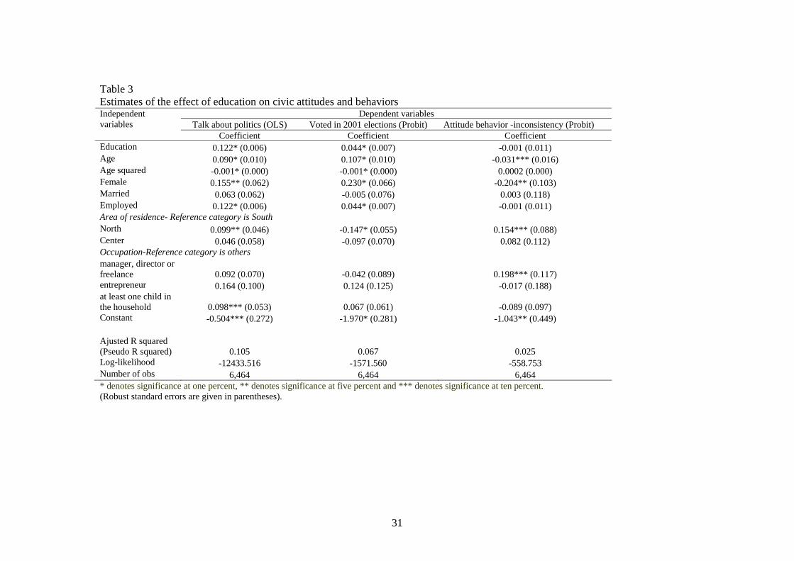
We first use the responses to the two questions above as dependent variables4 in
regressions with approximately the same explanatory factors included in the model
presented in Table 2.5 The estimates, which are depicted in the first and second columns
of Table 3, show that more educated individuals are more likely to talk about politics and
are also more likely to have voted, respectively. Thus it appears that education exerts a
significant positive influence not only on attitude towards politics but also on political
behavior. Next we use the attitude- behaviour inconsistency dummy as a dependent
variable in a probit model whose results are presented in the third column of Table 3.
Education is not systematically correlated with the probability of talking frequently about
politics but not having voted in 2001. This result may be interpreted as adding some
credibility to our empirical findings because it supports the hypothesis that the
discrepancy between civic opinions and congruent civic actions is randomly distributed
across educational levels.6
reported rather than validated voting data would not be led far astray in terms of what they conclude about the overall extent to which voting is related to demographic and political characteristics”. 4 For the first question, the order is reversed so high score indicates a higher political involvement. 5 Whilst we replace household income with a set of dummies for the individual’s occupation, number of children in the household is replaced with a dummy indicating the presence of at least once child in the household. Unfortunately there is no information on parental background or on urban location. 6 Some further support for our approach is also provided by Milligan et al. (2004). Using officially validated voting data they find that the bias associated with self-reported voting data is not a function of education, after controlling for a number of individual characteristics.
14
Insert Table 3 near here
Exclusion restriction
The estimates depicted in Table 2 may be biased because of the endogeneity of education.
In an attempt to address this problem, we use an IV method as well as a two-stage
ordered probit model. These methods typically require an instrument or an exclusion
restriction, which is a variable that affects education but has no impact on civic outcomes.
Following the approach of Flabbi (1999), we use two reforms of the Italian educational
system as an instrument for education.7 Both reforms can be viewed as exogenous events
that have contributed to remove barriers to participation in higher educational
opportunities, thereby raising the average educational levels of the Italian population. The
first reform (Law 1859, 31 December 1962) changed the organizational structure of
lower secondary school in an attempt to increase participation in upper secondary
education. Specifically, it established a single compulsory type of lower secondary school
that gives to the students who have successfully completed it the right to enrol at any type
of upper secondary school.8 The second educational reform (Law 910, 11 December 1969)
yielded an increase in participation in higher education by opening universities also to
those students successfully completing non-general upper secondary schools.9
7 A large number of studies use institutional features of the schooling system as an instrumental variable for education (for a review, see Card, 2001). 8 Before the reform there were two types of lower secondary school and one of them (i.e. scuola di avviamento professionale) had a strong vocational nature. Individuals who attended the latter were unlikely to continue their studies given that they could not enrol at general upper secondary schools and they had to pass an exam to be able to enrol at non-general upper secondary schools. 9 Before 1969 only those individuals successfully completing general upper secondary schools had automatic access to university.

15
As suggested by Flabbi (1999), considering that in Italy individuals usually begin lower
secondary school at the age of 12 and that the expected age of completion of upper
secondary school is, in general, 19 years, both the 1962 and the 1969 reforms are likely to
have affected the educational attainment of people born after 1950. This means that the
effect of these reforms can be captured through a single dummy variable that takes the
value 1 if the individual was born in 1951 or after, and 0 otherwise.10
The validity of the two-stage estimation strategy rests on the assumption that our
instrumental variable is not related to civic outcomes. This means that the 1962 and 1969
educational reforms should not be associated with other factors that, in turn, may affect
civic attitudes. At least one consideration supports this assumption. Civic courses, which
are found to be an important determinant of civic outcomes by several studies, were
introduced in Italy before these reforms. Specifically, they started in 1958 and since then
they have been compulsory and taught in lower secondary schools (scuole medie) as part
of the curriculum of classes in history (Sani, 2004).
In an attempt to analyze the effect of 1962 and 1969 reforms on educational attainment,
Figure 1 displays the proportion of individuals with at least an upper secondary school
diploma11 by year of birth. From this Figure it emerges that, on top of a general positive
trend in educational attainment, educational levels jumped for individuals born during the
10 The same dummy variable is used as an instrument by Brunello and Miniaci (1999) and Brunello et al. (2000). Additionally, this dummy is also employed by Checchi and Brunello (2005) as an explanatory factor in an educational attainment model. 11 We focus on these individuals as one would expect these reforms to increase the proportion of people who have either an upper secondary school diploma or a tertiary education degree.

16
beginning of the 1940s as well as for those born around 1950. The latter result may
possibly reflect the impact of these reforms.
Insert Figure 1 near here
Following the approach of Dee (2004), we employ a more formal method to test that our
instrument is “relevant” (i.e., correlated with education). Specifically, we estimate the
effects of the educational reforms on different levels of educational attainment using a
specification that includes a full set of controls. The OLS estimates, which are reported in
Table 4, provide support for the use of our instrument. In line with our expectations, these
estimates indicate that the effects associated with the educational reforms were
practically exclusively concentrated at the upper secondary/tertiary levels.
Insert Table 4 near here
Following the idea advanced by Card (1995) that accessibility matters more for
individuals on the margin of continuing their education, it is very likely that the 1962 and
1969 educational reforms had a differential effect, with larger increases in educational
attainment among people from less advantaged family backgrounds.12 Table 5 provides
some evidence supporting this hypothesis. It shows that increases in educational
attainment within the cohort born in 1951 or after are larger among those individuals who
12 A further consideration reinforces this conclusion. In Italy individuals from less advantaged family backgrounds tend to send their children to vocational/non-general secondary schools (Checchi and Flabbi, 2006). Before the 1962 and 1969 reforms this educational choice was significantly limiting their possibility to continue with further education.

17
have less-educated parents. For instance, whilst the proportion of individuals who,
despite having a father with no formal educational attainment, have at least an upper
secondary school diploma is 9.42 percent within the cohort born before 1951, the
corresponding figure is three times higher (i.e. 29.37 percent )within the cohort born in
1951 or after. This suggests that a possible specification of the first stage of the IV and
two-stage ordered probit models may include interactions of the reform dummy with
family background variables as instruments for schooling, in addition to the reform
dummy that is used as a direct control variable.13
Insert Table 5 near here
Two-stage estimates
This Section presents two-stage estimates in an attempt to account for the possibility that
education is endogenous to civic outcomes. Specifically, we use two different two-stage
procedures which only differ in the second stage estimation procedure. The first common
stage consists of an OLS regression where education is regressed on our instruments and
other covariates. In the second stage fitted values from this regression are then included
in the civic outcome equations instead of education. In line with the approach of Dee
(2004) and Milligan et al. (2004), we first estimate the second stage equation using OLS
following a standard IV process. However, to test the robustness of our findings and
13 Numerous studies (see, for instance, Card 1995) have used interactions between an institutional feature of the educational system and family background variables as instruments for schooling.

18
given the categorical nature of the dependent variables, this specification is also
estimated using an ordered probit model.14
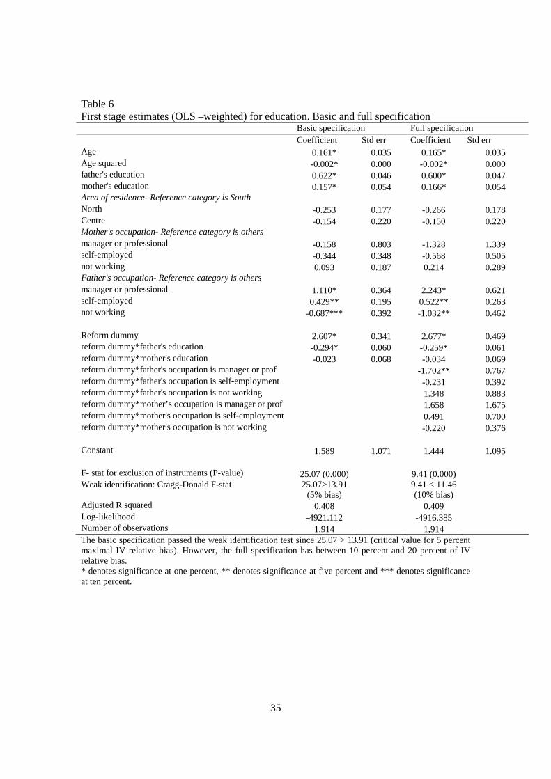
Table 6 reports the estimates for two alternative specifications of the first stage. The first
specification relies on a more parsimonious set of instruments that comprises the reform
dummy and interactions of the reform dummy with parental education. In the second
specification we add interactions of the reform dummy with parental occupation to our
set of instruments. This approach allows an examination of whether or not the estimates
are sensitive to the instruments employed to identify the model.
Insert Table 6 near here
These estimates show that those affected by the 1962 and 1969 educational reforms have
significantly higher educational attainment, conditioning on control variables such as
(among others) age15, gender, parental education and occupation. Specifically, the
findings indicate that these educational reforms increased years of schooling by a
statistically significant 2.61 years and 2.68 years in the first and specification
specifications, respectively.16 The coefficients on parental education and occupation
14 Given that years of education can be considered as a categorical variable, one may argue that other estimation techniques (e.g. ordered probit) than OLS would be more appropriate in the first stage. Nevertheless, Heckman (1978, p. 947) suggests that there is no loss in using OLS. In the light of this, several studies (see, for instance, Meer et al., 2003; Chun and Oh, 2002) employ an OLS regression in the first stage of a two-stage probit model. 15 Controlling for linear age and age squared variables is especially important as this ensures against the possibility that our reform dummy is simply picking up an upward drift in educational attainment. 16 If the reform dummy is included as the only instrument, the value of its coefficient (i.e. 0.91) is quite similar to that found by Brunello et al. (2000). However, following the approach of Denny and Harmon (2000), we do not report IV and two-stage ordered probit estimates based only on this instrument. When the

19
suggest that individuals from less advantaged backgrounds have lower education relative
to those from more advantaged backgrounds, other things being held constant. However,
in line with our expectations, the 1962 and 1969 reforms had the effect of reducing this
education inequality. For instance, whilst individuals whose father is a manager or a
professional have about 2.24 years more education than the default case of individuals
whose father has another occupation, after the reforms this disparity is reduced to
approximately 0.54 years.17
Next we check the explanatory power of our instrumental variables. Bound et al. (1995)
show that a weak correlation between the instruments and the endogenous variable may
make the two-stage estimation technique not to be superior of a simple regression where
there is no attempt to control for the endogeneity bias. Thus the correlation between our
set of instruments and education is checked using the F-statistic suggested by Staiger and
Stock (1997). This test, whose results are shown in Table 6, confirms that our instruments
are relevant as the F-statistic on the excluded instruments in the first stage is very high in
both specifications, thereby indicating that our identifying variables make a significant
contribution to explaining educational attainment.
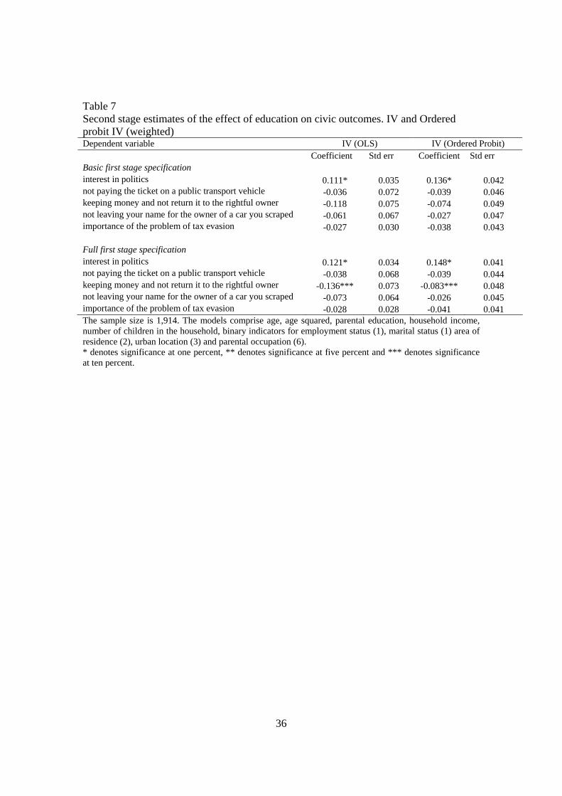
Table 7 depicts the estimates of the second stage of both the IV and the two-stage ordered
probit models. As regards the latter, consistent standard errors are computed using the
sample size is insufficiently large asymptotically efficiency is gained through the use of more instruments (Davidson and McKinnon, 1993). 17 A similar result is obtained by Denny and Harmon (2000).
20
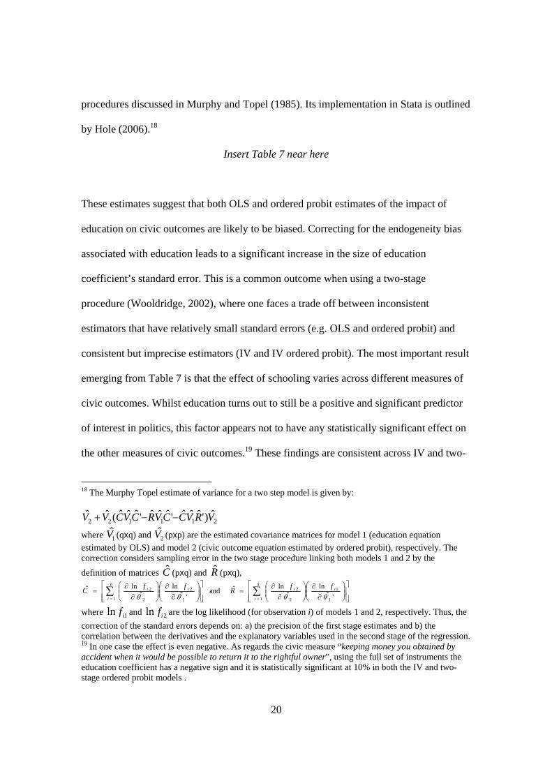
procedures discussed in Murphy and Topel (1985). Its implementation in Stata is outlined
by Hole (2006).18
Insert Table 7 near here
These estimates suggest that both OLS and ordered probit estimates of the impact of
education on civic outcomes are likely to be biased. Correcting for the endogeneity bias
associated with education leads to a significant increase in the size of education
coefficient’s standard error. This is a common outcome when using a two-stage
procedure (Wooldridge, 2002), where one faces a trade off between inconsistent
estimators that have relatively small standard errors (e.g. OLS and ordered probit) and
consistent but imprecise estimators (IV and IV ordered probit). The most important result
emerging from Table 7 is that the effect of schooling varies across different measures of
civic outcomes. Whilst education turns out to still be a positive and significant predictor
of interest in politics, this factor appears not to have any statistically significant effect on
the other measures of civic outcomes.19 These findings are consistent across IV and two-
18 The Murphy Topel estimate of variance for a two step model is given by:
211122ˆ)'ˆˆˆ'ˆˆˆ'ˆˆˆ(ˆˆ VRVCCVRCVCVV −−+
where 1V (qxq) and 2V (pxp) are the estimated covariance matrices for model 1 (education equation estimated by OLS) and model 2 (civic outcome equation estimated by ordered probit), respectively. The correction considers sampling error in the two stage procedure linking both models 1 and 2 by the definition of matrices C (pxq) and R (pxq),
⎥⎥⎦
⎤
⎢⎢⎣
⎡⎟⎟⎠
⎞⎜⎜⎝
⎛
∂∂
⎟⎟⎠
⎞⎜⎜⎝
⎛
∂∂
=⎥⎥⎦
⎤
⎢⎢⎣
⎡⎟⎟⎠
⎞⎜⎜⎝
⎛
∂∂
⎟⎟⎠
⎞⎜⎜⎝
⎛
∂∂
= ∑∑== 'ˆ
lnˆ
lnˆ and 'ˆ
lnˆ
lnˆ1
1
1 2
2
1
2
1 2
2
θθθθi
n
i
iin
i
i ffRffC
where 1ln if and 2ln if are the log likelihood (for observation i) of models 1 and 2, respectively. Thus, the correction of the standard errors depends on: a) the precision of the first stage estimates and b) the correlation between the derivatives and the explanatory variables used in the second stage of the regression. 19 In one case the effect is even negative. As regards the civic measure “keeping money you obtained by accident when it would be possible to return it to the rightful owner”, using the full set of instruments the education coefficient has a negative sign and it is statistically significant at 10% in both the IV and two-stage ordered probit models .
21
stage ordered probit estimates and are also consistent irrespective of the set of
instruments used. However, the specification with the full set of instruments delivers a
slightly more precise estimate of education (i.e. the estimated standard error are smaller).
Additionally, in line with the results obtained by Dee (2004) and Milligan et al. (2004),
our OLS and ordered probit estimates indicate that the omission of unobserved factors
leads to a downward bias in the estimated effect of education on political engagement.
However, the results depicted in Table 7 can be considered to be superior than those
reported in Table 2 only if education is found to be endogenous. In order to test for this,
we include the residual obtained from the first stage regression as an additional regressor
in the civic outcomes models whose results are presented in Table 2. If the coefficient on
the residual turns out to be statistically significant, this implies that education is
endogenous. Our findings from both the IV and two-stage ordered probit methods
indicate that, using the full set of instruments, the large majority of our measures of civic
outcomes are endogenous.20 Additionally, we use the Sargan misspecification test to
check the validity of our instruments, i.e. they should be orthogonal to the error term of
the civic outcomes equations. The results suggest that both our sets of instruments are
valid for all the civic outcomes IV models.21
Our findings imply the endogeneity bias associated with education can be either positive
or negative. On the one hand, since unobserved factors driving education are likely to be
20 In two cases education is found to be exogenous. The first one is with respect to “not paying the ticket on a public transport vehicle” in the IV method. The second one is with respect to “not leaving your name for the owner of a car you accidentally scraped” in the two-stage ordered probit model. 21 To save space, the results of the Hausman and Sargan tests are not reported.

22
negatively correlated with interest in politics, this causes a downward bias in the
estimated effect of schooling on this civic measure. On the other hand, since
unobservables that make individuals develop a taste for education are likely to be
positively correlated with the other measures of civic outcomes, the effect of education
tends to disappear once one accounts for the endogeneity bias.
Robustness checks
Two tests are performed to check the robustness of our two-stage estimates. First, we re-
estimate the civic outcome equations with some modifications in control variables (for
instance, it may be appropriate to drop martial status and family income as both these
variables are potentially endogenous). New IV and two-stage ordered probit estimates
confirm the robustness of our findings as the magnitude of the coefficients on education
is close to that reported in Table 7.22 Second, we conduct estimations on a subsample
which consists of individuals aged 33-73 in 2004. These individuals are selected in an
attempt to eliminate the effect of other factors potentially causing changes in the
educational attainment besides the 1962 and 1969 educational reforms. Thus, on the one
hand, we exclude those individuals whose educational attainment might have been
negatively affected by the WWII, i.e. individuals who were beyond compulsory
schooling age during or before the WWII. On the other hand, we also drop from the
sample those individuals who were 19 or younger in 1990 as their educational attainment
might have been positively influenced by the significant expansion of university supply
(Bratti et al., 2007). For this specific sub-sample, results are broadly consistent with those 22 Results are available from the authors upon request.

23
depicted in Table 7. Thus, the only civic measure affected by education once one controls
for the endogeneity bias is interest in politics, thought the size of the education
coefficients are slightly bigger than those in reported in Table 7 for both the IV and two-
stage ordered probit estimates.23
5. Conclusions
This paper has examined the casual effect of education on civic outcome in Italy. We
have attempted to extend previous research in this area by investigating the effect of
education on several measures of civic outcomes. Thus, in addition to political
engagement, which is a well-established proxy for civic outcomes, we have considered
other indicators capturing citizens’ opinion on a number of civic issues. We have
employed standard regression techniques such as OLS and ordered probit as well as IV
and two-stage ordered probit methods in an attempt to account for the endogeneity of
education.
23 Using the procedure employed by Altonji et al (2005), it is possible to compute the potential bias due to the use of a contaminated set of instruments with respect to the IV estimates of the effect of education on interest in politics. This bias results from the possibility that for a specific sub-sample our instruments are correlated with the residuals. To check whether this may be a problem in our analysis, the following equation is estimated for individuals aged either over 73 or under 33:
iFSii ZXY εδβα ++= )ˆ('
where Y is interest in politics, X is a vector of explanatory factors, Z is vector of instruments and FSβ is the estimated impact of the instruments in the first stage. Results from this regression show that the estimators of δ are not statistically significant, giving further support the results reported in Table 7 for the full sample.

24
In line with previous studies, our results show that the omission of unobserved factors
makes OLS and ordered probit estimates on education to be biased. However, we
conclude that the direction of this bias varies across different measures of civic outcomes.
On the one hand, we find that unobserved factors making individuals develop a taste for
education are likely to be negatively correlated with interest in politics. This implies that
the effect of education on interest in politics is likely to be underestimated if one does not
account for the endogeneity bias associated with education. On the other hand, since
unaccounted factors driving education are likely to be positively correlated with the other
civic measures examined in this study, the effect of education tends to disappear once one
controls for the endogeneity bias.
These results helps to reconcile various findings from previous studies (see, Dee, 2004
and Milligan et al., 2004 on the one hand and Gibson, 2001 on the other hand) showing
mixed results about the causal effect of education on civic outcomes.
25
References
Algan, Y., Cahuc, P., 2006. Civic attitudes and the design of labor market institutions: which countries can implement the Danish flexicurity model?. IZA Discussion Paper No. 1928. Altonji, J. G., Elder, T.E., Taber, C.R., 2005. An Evaluation of Instrumental Variable Strategies for Estimating the Effects of Catholic Schooling. Journal of Human Resources 40, 791-821. Bound, J., Jaeger, D., Baker, R., 1995. Problems with the instrumental variable estimation when the correlation between the instruments and the endogenous explanatory variable is weak. Journal of the American Statistical Association 90, 443-450. Bratti, M., Checchi, D., De Blasio, G., 2007. The impact of higher education supply on schooling: Evidence from Italy’s university devolution. Paper presented at the 2007 Annual Conference of the European Labour Economic Association, Oslo. Brunello, G., Miniaci, R., 1999. The economic returns to schooling for Italian men. An evaluation based on instrumental variables. Labour Economics 6, 509-519. Brunello, G., Comi, S., Lucifora C., 2000. The returns to education in Italy: a new look at the evidence. IZA Discussion Papers No. 130. Brunello, G., Checchi, D., 2005. School quality and family background in Italy. Economics of Education Review 24, 563-577. Campbell, D. E. 2006. What is education’s impact on civic and social engagement? Paper presented at the Symposium on Social Outcomes of Learning. Danish University of Education, Copenhagen. Card, D., 1995. Using geographical variation in college proximity to estimate the return to schooling. In Christofides L.N., Grant E.K., Swidinsky, R. (Eds.). Aspects of Labour Market Behaviour: Essay in Honour of John Vanderkamp, University of Toronto Press. Card, D., 2001. Estimating the return to schooling: progress and some persistent econometric problems. Econometrica 69, 1127-1160. Chun, H., Oh, J., 2002. An instrumental variable estimate of the effects of fertility on the labour force participation of married women. Applied Economics Letters 9, 631-634. Checchi, D., Flabbi, L., 2006. Intergenerational mobility and schooling decisions in Italy and Germany. Paper presented at the 2006 Annual Conference of the European Economic Association, Vienna.

26
Davidson, R., and McKinnon J.G., 1993 Estimation and Inference in Econometrics. New York: Oxford University Press. Dee, T.S., 2004. Are there any returns to civic education?. Journal of Public Economics 88, 1697-1720. Denny, K.J., Harmon, C.P., 2000. Education policy reform and the returns to schooling from instrumental variables. The Institute of Fiscal Studies WP 00/07. Ehman, L.H., 1980. The American school in the political socialization process. Review of Educational Research 50, 99-119. Flabbi L., 1999. Returns to Schooling in Italy: OLS, IV and Gender Differences. Bocconi University Working Paper No. 1. Gibson, J., 2001. Unobservable family effects and the apparent external benefits of education. Economics of Education Review 20, 225-233 Heckman, J.J., 1978. Dummy endogenous variables in a simultaneous equation system. Econometrica 46, 931-953. Hole, A., 2006. Calculating Murphy–Topel variance estimates in Stata: A simplified procedure. The Stata Journal 6, 521–529. Ichino, A., Maggi, G., 2000. Work Environment and Individual Background: Explaining Regional Shirking Differentials in a Large Italian Firm. Quarterly Journal of Economics 115, 1057-1090. Ichino, A., Winter-Ebmer, R., 2004. The Long-Run Educational Cost of World War Two. Journal of Labor Economics 22, 57-86. Langton, K.P., Jennings, M.K., 1968. Political socialisation and the high school civics curriculum in the United States. American Political Science Review 62, 852-867. Leming, J.S., 1983. Research on social studies curriculum and instruction: interventions and outcomes in the socio-moral domain. In Stanley W.B., (Ed.) Review of Research on Social Studies Education: 1976-1983, Washington, DC: National Council for the Social Studies. Meer, J., Miller, D.L., Rosen, H.S., 2003. Exploring the health-wealth nexus, Journal of Health Economics 22, 713-730. Miller, J.D., 1985. Effective participation: a standard for social studies education. Paper presented at the Annual Meeting of Social Science Education Consortium. Racine. Wisconsin.

27
Milligan, K., Moretti, E., Oreopoulos, P., 2004. Does education improve citizenship? Evidence from the United States and the United Kingdom. Journal of Public Economics 88, 1667-1695. Murphy, K., Topel, R., 1985. Estimation and inference in two-step econometric models. Journal of Business and Economic Statistics 3, 370-379. Niemi, R.G., Junn, J., 1998. Civic education: what makes students learn?. New Haven: Yale University Press.
Sani, R., 2004. La scuola e l’educazione alla democrazia negli anni del secondo dopoguerra. In Corsi, M., Sani, R., (Eds). L’educazione alla democrazia tra passato e presente, Milano: Vita e Pensiero, 43-62.
Sigelman, L., 1982. The nonvoting voter research. American Journal of Political Science 261, 47-56.
Silver, B.D., Anderson, B.A., Abramson, P.R., 1986.Who overreports voting?. American Political Science Review 80, 613-624. Smith, E.S., 1999. The effects of investment in social capital of youth on political and civic behaviour in young adulthood: a longitudinal analysis. Political Psychology 20, 553-580. Schlozman, K.L., Burns, N., Verba, S., 1994. Gender and the pathways to participation; the role of resources. The Journal of Politics 56. 963-990. Staiger, D., Stock, J.H., 1997. Instrumental variable regression with weak instruments. Econometrica 65, 557-586. Torney-Purta, J., 2002. The school’s role in developing civic engagement: a study of adolescents in twenty-eight countries. Applied Developmental Science 6, 202-211. Vieira, J.A.C., 1999. Returns to education in Portugal.. Labour Economics 6, 535-541. Wolfinger, R.E., Rosentone, S.J., 1980. Who votes?. Yale University Press, New Haven, Connecticut. Wooldridge, J., 2002. Econometric Analysis of Cross Section and Panel Data. Cambridge, MA: MIT Press.

28
Table 1 Descriptive statistics
Variables Mean Standard Deviation
Education (years of schooling) 9.50 4.23 Civic outcomes Interest in politics 2.04 0.92 Not paying the ticket on a public transport vehicle 8.78 1.96 Keeping money and not return it to the rightful owner 8.84 1.96 Not leaving your name for the owner of a car you scraped 8.96 1.88 Importance of the problem of tax evasion 4.12 0.80 Household income (euro) 35078.39 38001.83 Age (years) 55.54 14.62 Age squared (years) 3298.16 1624.95 Father's education (years of schooling) 5.03 4.09 Mother's education (years of schooling) 4.10 3.57 Married=1 0.81 0.39 Employed=1 0.53 0.50 Number of children in the household 0.86 0.98 Area of residence North=1 0.47 0.50 South=1 0.29 0.45 Centre=1 0.24 0.43 Urbanization Small town (below 20,000 inhabitants)=1 0.31 0.46 Medium-sized town (between 20,000 and 40,000 inhabitants)=1 0.20 0.40 Big town (between 40,000 and 500,000 inhabitants)=1 0.40 0.49 Very big town (above 500,000 inhabitants)=1 0.08 0.28 Mother's occupation Manager or professional 0.01 0.09 Self-employed 0.07 0.26 Not working 0.71 0.45 Others 0.21 0.41 Father's occupation Manager or professional 0.05 0.22 Self-employed 0.21 0.41 Not working 0.04 0.20 Others 0.69 0.46 Reform dummy =1 0.45 0.50 Number of observations 1,914
29
Table 2 OLS and Ordered Probit estimates (weighted) Independent variables
OLS Ordered Probit
Interest in politics
Not paying the ticket on a public vehicle
Keeping money and not return it to the owner
Not leaving your name for the owner of a car you scraped
Importance of the problem of tax evasion
Interest in politics
Not paying the ticket on a public vehicle
Keeping money and not return it to the owner
Not leaving your name for the owner of a car you scraped
Importance of the problem of tax evasion
Age 0.031* 0.070* 0.017 0.029 0.032* 0.041* 0.043* 0.016 0.027** 0.046* (0.010) (0.021) (0.021) (0.020) (0.009) (0.012) (0.013) (0.013) (0.013) (0.012) Age squared -0.000* -0.000** -0.000 -0.000 -0.000* -0.000* -0.000** -0.000 -0.000 -0.000* (0.000) (0.000) (0.000) (0.000) (0.000) (0.000) (0.000) (0.000) (0.000) (0.000) Education 0.071* 0.052* 0.026*** 0.035* 0.026* 0.087* 0.048* 0.026* 0.036* 0.037* (0.006) (0.014) (0.014) (0.013) (0.006) (0.008) (0.009) (0.009) (0.009) (0.008) father's education -0.022** -0.021 0.022 0.021 -0.003 -0.027** -0.017 0.023*** 0.009 -0.004 (0.009) (0.019) (0.019) (0.017) (0.008) (0.011) (0.012) (0.012) (0.012) (0.011) mother's education 0.012 0.019 0.010 -0.003 0.017** 0.016 0.020 -0.000 0.006 0.026** (0.009) (0.020) (0.020) (0.019) (0.008) (0.012) (0.013) (0.013) (0.013) (0.012) married 0.053 -0.127 -0.167 -0.356* 0.115** 0.065 -0.054 -0.038 -0.205* 0.170** (0.056) (0.121) (0.121) (0.112) (0.049) (0.071) (0.075) (0.077) (0.079) (0.071) employed 0.021 0.120 -0.095 -0.001 -0.017 0.021 0.052 -0.141 -0.080 -0.029 (0.063) (0.136) (0.136) (0.126) (0.055) (0.080) (0.085) (0.087) (0.088) (0.081) Number of children in the household -0.093* 0.008 0.087 0.122** -0.014 -0.119* 0.001 0.006 0.062*** -0.015 (0.025) (0.054) (0.054) (0.050) (0.022) (0.032) (0.034) (0.035) (0.035) (0.032) household income 0.000002* 0.000003*** 0.000004* 0.000002*** 0.00000 0.000002** 0.000003** 0.000005* 0.000002*** 0.00000 (0.000001) (0.000001) (0.000001) (0.000001) (0.000001) (0.000001) (0.000001) (0.000001) (0.000001) (0.000001)
30
Table 2- continued Area of residence- Reference category is South North -0.017 0.693* 0.631* 0.820* 0.060 -0.016 0.330* 0.314* 0.447* 0.079 (0.050) (0.107) (0.107) (0.099) (0.044) (0.063) (0.067) (0.068) (0.068) (0.064) Centre -0.067 0.538* 0.189 0.441* 0.172* -0.076 0.189** 0.012 0.214* 0.265* (0.061) (0.132) (0.132) (0.122) (0.054) (0.078) (0.082) (0.082) (0.083) (0.079) Urbanization- Reference category is very big town small town -0.078 -0.025 0.096 0.184 0.115*** -0.098 -0.023 0.130 0.118 0.177** (0.067) (0.144) (0.144) (0.134) (0.059) (0.084) (0.091) (0.091) (0.093) (0.085) medium-sized town -0.148*** 0.191 0.188 0.177 0.162** -0.188*** 0.175 0.195*** 0.136 0.236** (0.078) (0.168) (0.168) (0.156) (0.069) (0.099) (0.107) (0.107) (0.109) (0.100) big town 0.045 -0.190 -0.143 -0.032 0.189* 0.055 -0.128 -0.050 -0.035 0.280* (0.070) (0.150) (0.150) (0.139) (0.061) (0.087) (0.094) (0.094) (0.096) (0.089) Mother's occupation- Reference category is others manager or prof 0.241 -0.730 0.063 -0.485 -0.243 0.253 -0.542*** -0.227 -0.652** -0.385 (0.220) (0.472) (0.471) (0.437) (0.192) (0.272) (0.286) (0.291) (0.284) (0.276) self-employed 0.038 0.463** 0.417** 0.206 -0.046 0.030 0.260** 0.227*** 0.045 -0.059 (0.095) (0.204) (0.204) (0.189) (0.083) (0.120) (0.131) (0.131) (0.132) (0.122) not working -0.099*** 0.072 0.356* 0.023 -0.097** -0.136** 0.024 0.177* -0.036 -0.134** (0.051) (0.109) (0.109) (0.101) (0.044) (0.064) (0.067) (0.068) (0.070) (0.065) Father's occupation- Reference category is others manager or prof 0.080 0.074 -0.090 -0.042 -0.216** 0.097 0.060 0.002 0.045 -0.304** (0.100) (0.214) (0.214) (0.198) (0.087) (0.124) (0.139) (0.142) (0.144) (0.126) self-employed -0.049 0.064 0.174 0.117 -0.043 -0.048 -0.004 0.081 0.010 -0.065 (0.053) (0.115) (0.114) (0.106) (0.047) (0.068) (0.072) (0.073) (0.073) (0.068) not working 0.025 0.100 -0.059 -0.024 -0.083 0.045 0.015 -0.089 0.020 -0.131 (0.107) (0.230) (0.230) (0.213) (0.094) (0.136) (0.143) (0.145) (0.151) (0.135) Constant 0.609** 5.370* 7.103* 6.976* 2.592* (0.271) (0.582) (0.581) (0.538) (0.237) R-squared adjusted (Pseudo R-squared) 0.109 0.059 0.044 0.060 0.052 0.049 0.029 0.025 0.028 0.028 Log-likelihood -2432.156 -3896.323 -3893.251 -3748.274 -2174.589 -2279.982 -2689.822 -2547.569 -2399.648 -2086.864 Number of obs 1,914 1,914 1,914 1,914 1,914 1,914 1,914 1,914 1,914 1,914 *denotes significance at one percent, **denotes significance at five percent and ***denotes significance at ten percent. (Standard errors are given in parentheses).
31
Table 3 Estimates of the effect of education on civic attitudes and behaviors
Dependent variables Talk about politics (OLS) Voted in 2001 elections (Probit) Attitude behavior -inconsistency (Probit)
Independent variables
Coefficient Coefficient Coefficient Education 0.122* (0.006) 0.044* (0.007) -0.001 (0.011) Age 0.090* (0.010) 0.107* (0.010) -0.031*** (0.016) Age squared -0.001* (0.000) -0.001* (0.000) 0.0002 (0.000) Female 0.155** (0.062) 0.230* (0.066) -0.204** (0.103) Married 0.063 (0.062) -0.005 (0.076) 0.003 (0.118) Employed 0.122* (0.006) 0.044* (0.007) -0.001 (0.011) Area of residence- Reference category is South North 0.099** (0.046) -0.147* (0.055) 0.154*** (0.088) Center 0.046 (0.058) -0.097 (0.070) 0.082 (0.112) Occupation-Reference category is others manager, director or freelance 0.092 (0.070) -0.042 (0.089) 0.198*** (0.117) entrepreneur 0.164 (0.100) 0.124 (0.125) -0.017 (0.188) at least one child in the household 0.098*** (0.053) 0.067 (0.061) -0.089 (0.097) Constant -0.504*** (0.272) -1.970* (0.281) -1.043** (0.449) Ajusted R squared (Pseudo R squared) 0.105 0.067 0.025 Log-likelihood -12433.516 -1571.560 -558.753 Number of obs 6,464 6,464 6,464 * denotes significance at one percent, ** denotes significance at five percent and *** denotes significance at ten percent. (Robust standard errors are given in parentheses).

32
Figure 1: Fraction of individuals with at least an upper secondary school diploma 0
.2.4
.6.8
1
1910 1920 1930 1940 1950 1960 1970 1980year of birth
bandwidth = .15
Note: The y axis represents a weighted mean of individuals who have either an upper secondary school diploma or a tertiary education degree.

33
Table 4 OLS estimates (weighted) of the effect of educational reforms on measures of educational attainment Dependent variable Coefficient No educational attainment 0.005(0.013) Primary school -0.122*(0.030) Lower secondary school 0.024(0.034) Upper secondary school/tertiary education 0.093**( 0.037)
The sample size is 1,914. The models comprise age, age squared, parental education, binary indicators for area of residence (2) and parental occupation (6). Standard errors are given in parentheses. *denotes significance at one percent, **denotes significance at five percent and ***denotes significance at ten percent.

34
Table 5 Proportion of individuals with at least an upper secondary school diploma by parental education and by cohort of birth (percentage) Before 1951 In 1951 or after Father's education No formal educational attainment 9.42 29.37 Primary school certificate 32.72 47.94 Lower secondary school diploma 77.92 72.99 At least upper secondary school diploma 94.12 87.31 Mother's education No formal educational attainment 13.16 38.30 Primary school certificate 40.46 52.34 Lower secondary school diploma 83.67 71.05 At least upper secondary school diploma 96.15 92.00
35
Table 6 First stage estimates (OLS –weighted) for education. Basic and full specification Basic specification Full specification Coefficient Std err Coefficient Std err Age 0.161* 0.035 0.165* 0.035 Age squared -0.002* 0.000 -0.002* 0.000 father's education 0.622* 0.046 0.600* 0.047 mother's education 0.157* 0.054 0.166* 0.054 Area of residence- Reference category is South North -0.253 0.177 -0.266 0.178 Centre -0.154 0.220 -0.150 0.220 Mother's occupation- Reference category is others manager or professional -0.158 0.803 -1.328 1.339 self-employed -0.344 0.348 -0.568 0.505 not working 0.093 0.187 0.214 0.289 Father's occupation- Reference category is others manager or professional 1.110* 0.364 2.243* 0.621 self-employed 0.429** 0.195 0.522** 0.263 not working -0.687*** 0.392 -1.032** 0.462 Reform dummy 2.607* 0.341 2.677* 0.469 reform dummy*father's education -0.294* 0.060 -0.259* 0.061 reform dummy*mother's education -0.023 0.068 -0.034 0.069 reform dummy*father's occupation is manager or prof -1.702** 0.767 reform dummy*father's occupation is self-employment -0.231 0.392 reform dummy*father's occupation is not working 1.348 0.883 reform dummy*mother’s occupation is manager or prof 1.658 1.675 reform dummy*mother's occupation is self-employment 0.491 0.700 reform dummy*mother's occupation is not working -0.220 0.376 Constant 1.589 1.071 1.444 1.095 F- stat for exclusion of instruments (P-value) 25.07 (0.000) 9.41 (0.000) Weak identification: Cragg-Donald F-stat 25.07>13.91
(5% bias) 9.41 < 11.46 (10% bias)
Adjusted R squared 0.408 0.409 Log-likelihood -4921.112 -4916.385 Number of observations 1,914 1,914 The basic specification passed the weak identification test since 25.07 > 13.91 (critical value for 5 percent maximal IV relative bias). However, the full specification has between 10 percent and 20 percent of IV relative bias. * denotes significance at one percent, ** denotes significance at five percent and *** denotes significance at ten percent.
36
Table 7 Second stage estimates of the effect of education on civic outcomes. IV and Ordered probit IV (weighted) Dependent variable IV (OLS) IV (Ordered Probit) Coefficient Std err Coefficient Std err Basic first stage specification interest in politics 0.111* 0.035 0.136* 0.042 not paying the ticket on a public transport vehicle -0.036 0.072 -0.039 0.046 keeping money and not return it to the rightful owner -0.118 0.075 -0.074 0.049 not leaving your name for the owner of a car you scraped -0.061 0.067 -0.027 0.047 importance of the problem of tax evasion -0.027 0.030 -0.038 0.043 Full first stage specification interest in politics 0.121* 0.034 0.148* 0.041 not paying the ticket on a public transport vehicle -0.038 0.068 -0.039 0.044 keeping money and not return it to the rightful owner -0.136*** 0.073 -0.083*** 0.048 not leaving your name for the owner of a car you scraped -0.073 0.064 -0.026 0.045 importance of the problem of tax evasion -0.028 0.028 -0.041 0.041 The sample size is 1,914. The models comprise age, age squared, parental education, household income, number of children in the household, binary indicators for employment status (1), marital status (1) area of residence (2), urban location (3) and parental occupation (6). * denotes significance at one percent, ** denotes significance at five percent and *** denotes significance at ten percent.