Embed Size (px)
Citation preview

1
Determinants of Capital Structure of Firms in the Manufacturing Sector of Firms
in Indonesia
Dissertation
To obtain the degree of
Doctor of Business Administration
at the Maastricht School of Management,
under authority of the Dean Director Prof. dr. Peter P. de Gijsel
to be defended in public on May, 2012
by
Siti Rahmi Utami
born in Jakarta (Indonesia)

2
Published by:
Maastricht School of Management
P.O. Box 1203
6201 BE Maastricht
The Netherlands
Siti Rahmi Utami, Determinants of Capital Structure of Firms in the Manufacturing Sector of
Firms in Indonesia. DBA Dissertation, Maastricht School of Management, Maastricht 2012. –
With references. – With summary in English.
Key words: Capital Structure/Pecking Order Theory/Trade-off Theory/Firm Life Cycle/Signalling
Theory/Asymmetric Information/Agency Cost Theory
ISBN:
Cover: Stoerebinken, The Netherlands
Printing: Gildeprint, The Netherlands
© 2012 by Siti Rahmi Utami, Maastricht School of Management. All rights reserved. No part of
this publication may be reproduced, stored in a retrieval system or transmitted in any form or by
any means, electronic, mechanical, photocopying, recording or otherwise, without prior written
permission of the publisher.

3
This dissertation is approved of by the Doctoral Supervisor:
Prof. Eno L. Inanga
Maastricht School of Management, The Netherlands
Composition of the Evaluation Committee:
Prof. Dr. Ir. E. J. de Bruijn
Twente University, The Netherlands
Prof. Dr. Geert Braam RA

4
ACKNOWLEDGEMENTS
It is with a lot of gratitude and appreciation that I acknowledge the help of my supervisor,
Professor Eno L. Inanga, who has helped me to complete this Draft DBA thesis. The Draft DBA
thesis would not have reached this stage in the present form without his help. He has given me
support throughout the entire process. I am hugely indebted to him for all the hours he spent
reading my texts, writing suggestions and comments for me, and helping me to shape my thinking
in many ways. I greatly appreciate his expertise in the field of my research.
Likewise, I would also like to express my gratefulness to Professor Dadan, from Trisakti
University, Indonesia, for his encouragement and guidance. I also owe many thanks to the
administrative support I enjoyed from the Doctoral Office at MSM, as well as the administration
office at TIBS, Indonesia, are worthy of a mention with special thanks.
I must express my profound thanks to my parents (especially my father, Professor Gani
SH), without their support, I would not have achieved this stage. Last, but not least, I would also
like to thank to my friends, I have learned many things from them.

5
TABLE OF CONTENTS
ACKNOWLEDGEMENTS ................................................................................................................ 4
EXECUTIVE SUMMARY ................................................................................................................. 9
1. INTRODUCTION ....................................................................................................................... 11
1.1 Background of the Research ............................................................................................... 11
1.1.1. The Importance of Capital Structure Theory........................................................................ 11
1.1.2. Research Motivation ............................................................................................................. 15
1.2 Problem Identification .............................................................................................................. 17
1.3 Research Questions .................................................................................................................. 19
1.3.1 Major Research Questions .................................................................................................... 19
1.3.2 Minor Research Questions .................................................................................................... 19
1.4 Research Objectives ................................................................................................................. 20
1.5 Scope and Limitation of the Study ............................................................................................ 20
1.6 Expected Contribution .............................................................................................................. 22
1.7 Organisation of the Study ......................................................................................................... 23
2. AN OVERVIEW OF THE CAPITAL STRUCTURE OF INDONESIAN MANUFACTURING
FIRMS ............................................................................................................................................ 24
2.1. Indonesian Capital Market ...................................................................................................... 24
2.1.1 History of Indonesia Stock Exchange .................................................................................... 24
2.1.2 Stock Price Index in the Indonesian Capital Market ............................................................. 24
2.1.3. Description of the LQ45 Index ............................................................................................. 26
2.2. Characteristics of the Research Sample .................................................................................. 26
2.3 Leverage Analysis ..................................................................................................................... 34
3. LITERATURE REVIEW .............................................................................................................. 36
3.1 Theories of Capital Structure ................................................................................................... 36
3.1.1 Modigliani-Miller Theory ...................................................................................................... 36
3.1.2. The Capital Structure Theory ............................................................................................... 37
3.2. The Conclusions What Variables We Use for Our Research, and Why These, Theories
Predictions of the Relationship between Variables, and Some Previous Research Findings ......... 40
3.2.1 Selected Variables regarding Capital Structure for Research Question 1a, 1b, 1c, 1d, and 1e 40

6
3.2.2 Selected Variables for Research Question 2 .......................................................................... 46
3.2.3 Selected Variables for Research Question 3a, 3b, and 3c ..................................................... 48
3.2.4 Selected Variables for Research Question 4 .......................................................................... 51
4. CONCEPTUAL FRAMEWORK ................................................................................................. 54
4.1 Conceptual Framework for Research Question 1a, 1b, 1c, 1d, and 1e .................................... 54
4.1.1 Previous Research regarding Capital Structure Determinants ............................................. 54
4.1.2 Conceptual Framework for Research Question 2 ................................................................. 65
4.1.3 Conceptual Framework for Research Question 3 ................................................................. 68
4.1.4 Conceptual Framework for Research Question 4 ................................................................. 72
5. RESEARCH METHODOLOGY.................................................................................................. 76
5.1 Research Design ....................................................................................................................... 76
5.2Research Strategy ...................................................................................................................... 77
5.2.1. Quantitative Strategy ............................................................................................................ 77
5.2.2. Mixed Method Strategy ......................................................................................................... 78
5.3 Data Collection ........................................................................................................................ 78
5.4. Sampling Design and Procedure ............................................................................................. 79
5.5. Variables Measurement ........................................................................................................... 80
5.5.1. Variable of Hypothesis 1 ...................................................................................................... 80
5.5.2 Measuring Variables of Hypotheses 2, 3, and 4 .................................................................... 82
5.6. Hypotheses Testing ................................................................................................................... 83
5.6.1. Hypothesis 1 .......................................................................................................................... 84
5.6.2. Hypothesis 2 ......................................................................................................................... 84
5.6.3. Hypothesis 3 ......................................................................................................................... 86
5.6.4. Hypothesis 4 ......................................................................................................................... 86
5.7. Regression Analysis ................................................................................................................. 91
A. The Un-standardised Beta Coefficients ..................................................................................... 91
B. The Standardised Beta Coefficients ........................................................................................... 91
C. Analysis of Variance (ANOVA).................................................................................................. 91
D. The Coefficient of Determination (R2) ....................................................................................... 91
E. Descriptive Statistics .................................................................................................................. 92
F. Regression Assumptions of Hypothesis 1-4 ................................................................................ 92
5.8. The Credibility of Research Findings ...................................................................................... 94
7
5.8.1 Reliability .............................................................................................................................. 94
5.8.2 Validity .................................................................................................................................. 94
5.8.3 Generalisability ..................................................................................................................... 94
5.9. The Limitations of Research Design ........................................................................................ 94
6. PRESENTATION OF DATA AND ANALYSIS OF RESULTS .................................................... 96
6.1 Research Question 1, Hypotheses, Hypotheses Testing, and Result Analysis .......................... 96
6.1.1. Research Question 1 ............................................................................................................. 96
6.1.2. Hypothesis One (H1) ............................................................................................................ 96
6.1.3. Testing the Hypothesis 1 ....................................................................................................... 97
6.1.4. Analysis of Results ................................................................................................................ 97
6.2. Research Question 2, Hypothesis 2, Hypothesis Testing, and Result Analysis ...................... 111
6.2.1. Research Question 2 ........................................................................................................... 111
6.2.2. Hypothesis 2 ....................................................................................................................... 111
6.2.3. Testing the Hypothesis 2 ..................................................................................................... 111
6.2.4. Analysis of Quantitative Results of Hypothesis 2 ............................................................... 112
6.2.5 Qualitative Analysis of Hypothesis 2 ................................................................................... 117
6.3. Research Question 3, Hypothesis, Hypothesis Testing, and Result Analysis ........................ 129
6.3.1. Research Question Three .................................................................................................... 129
6.3.2. Hypothesis 3 ....................................................................................................................... 129
6.3.3. Testing the Hypothesis 3 ..................................................................................................... 130
6.3.4. Analysis of Results .............................................................................................................. 130
6.4. Research Question 4, Hypothesis, Hypothesis Testing, and Result Analysis ......................... 137
6.4.1. Research Question 4 ........................................................................................................... 137
6.4.2. Hypothesis 4 ....................................................................................................................... 137
6.4.3. Testing Hypothesis 4 ........................................................................................................... 137
6.4.4 Sample Description ............................................................................................................. 138
6.4.5. Analysis of Results .............................................................................................................. 139
6.4.6. Capital Structure over Firm’s Life Cycle ........................................................................... 148
6.4.7 Frequency ............................................................................................................................ 151
6.5. Statistical Power Analysis of Hypotheses 1, 2, 3, and 4 ........................................................ 157
6.6. Regression Assumptions of Hypotheses 1, 2, 3, and 4 ........................................................... 163
1. Multicollinearity ....................................................................................................................... 163
2. Autocorrelation ........................................................................................................................ 165

8
3. Heteroscedasticity .................................................................................................................... 166
4. Normally Distributed ................................................................................................................ 166
6.7. Results of Panel Data Regression Analysis and the Comparison to Regression Analysis .... 166
7. CONCLUSION ......................................................................................................................... 170
7.1. Conclusion ............................................................................................................................. 170
7.2 Conclusion regarding Result and Its Consistency with Condition of Indonesian Capital Market
171
7.3. To What Extent is the Study Scientifically Relevance ............................................................ 174
7.4. Recommendations and Suggestions for Further Research .................................................... 175
7.5. Suggestions for Managers ..................................................................................................... 176
7.6. Managerial Implication ......................................................................................................... 176
BIBLIOGRAPHY .......................................................................................................................... 177
APPENDIX ................................................................................................................................... 186
APPENDIX A ............................................................................................................................... 186
APPENDIX B ............................................................................................................................... 206
APPENDIX C ............................................................................................................................... 213
APPENDIX D ............................................................................................................................... 220
APPENDIX E ............................................................................................................................... 241

9
EXECUTIVE SUMMARY
The objectives of this research are: to investigate the determinants of capital structure of
the firms in the manufacturing sector in Indonesian capital market; to analyse how firms in the
manufacturing sector raise capital for investments, internally or externally (with debt, equity, or
debt to repurchase equity); to examine if debt policy does matter; what will happen to the firm‟s
stock price if firms issue new debt, issue new equity, or issue debt to repurchase equity; and to
examine within the context of a firm‟s life cycle whether we can expect that growth-small firms
follow the pecking order more closely than mature-large firms. Therefore, we examine 4 major
hypotheses. By using regression analysis we test all hypotheses, while for hypothesis 2 we use
qualitative analysis, too, and for hypotheses 2 and 4 we also apply an augmented model.
Overall, our results showed that under the linear regression model, firms exhibit as
follows. For hypothesis 1, profitability has a negative significant regression coefficient on short-
term leverage; long-term leverage; total leverage, and on market leverage. Tangibility has a
negative significant regression coefficient on short-term leverage, while tangibility has a positive
significant regression coefficient on long-term and market leverage. Tangibility also has a positive
but not significant regression coefficient on total leverage.
Size, has a positive, yet not significant regression coefficient on short-term leverage and
total leverage, while size has a negative, yet not significant regression coefficient on long-term
leverage, and size has a negative significant regression coefficient on market leverage. Risk has a
positive significant regression coefficienton short-term leverage and total leverage while risk has a
negative significant regression coefficient on long-term leverage. Risk also has a positive but not
significant regression coefficient on market leverage. Growth has a positive significant regression
coefficient on short-term, long-term, and total leverage; however, growth has a negative
significant regression coefficient on market leverage.
For hypothesis 2, we can conclude that the financing deficit has positive significant
effects on the net debt issue and on net equity issue. This result suggests that high deficit firms
would tend to issue more net debt and net equity to finance their financing deficit. The financing
deficit has negative, yet not significant effects on newly retained earning. This result suggests that
high deficit firms would not tend to use newly retained earning to finance the financing deficit.
The financing deficit has negative, but not significant effects on repurchase equity. This result
suggests that high deficit firms would not tend to repurchase equity to finance the financing
deficit. From the descriptive table, we see that the amount of net debt issue is more than net equity
issue and it is consistent with regression results.
For the augmented model, our result shows a positive coefficient on the financial deficit
and also on the squared deficit term. However, for the squared deficit term, the coefficient was not
significant. Therefore, we conclude that our firm sample firm prefers external to internal financing
and debt to equity if external financing is used.
For hypothesis 3, the results indicate that net debt has no positive significant impact on
the stock price of from January to December and on the yearly stock price. Net equity has no
negative significant impact on the stock price from January to December and on the yearly stock
price. This result suggests that firms that issue more net equity would tend to have decreasing

10
stock price, while issuing more net debt, the firm would tend to have increasing stock price. The
result also suggests that firms repurchasing equity would tend to have increasing monthly and
yearly stock price.
For hypothesis 4, the growth firms, we conclude that the financing deficit has positive
significant effects on the net debt issue and on the net equity issue, and financing deficit has
negative significant effects on newly retained earning. For mature firms, we conclude that the
financing deficit has positive significant effects on the net debt issue and the net equity issue,
while a financing deficit has negative insignificant effects on newly retained earning. From these
results, we conclude that our mature and growth firm prefers external to internal financing and
debt to equity if external financing is used. Overall, we find that the pecking order theory describes
the financing patterns of growth firms better than mature firms.
11
1. INTRODUCTION
1.1 Background of the Research
1.1.1. The Importance of Capital Structure Theory
At the time a firm faces a financial deficit that affects its financial condition, the manager
of the firm should be able to make a managerial decision as well as a financial decision in order to
maintain the viability of the firm. One way that can be chosen is to undertake a capital
restructuring, especially debt restructuring. The decision taken on debt restructuring, of course,
requires expertise and analystic capabilities so managers can make the right decisions of financial
restructuring for the company. An ideal composition of capital structure which consists of debt and
equity, will minimise the cost of capital and maximise the firm‟s value. Therefore, it is important
for the firm‟s manager to understand the theory of capital structure.
The sources of funds include retained earnings, debt, and equity. Retained earning is the
cheapest fund for the funding source as it does not have explicit costs in the same way as funds
obtained from outside sources. When the company uses debt to finance investments which has an
impact on costs rising in its capital structure, the company will have a financial risk, because the
company must consider their priority in the structure of debt, debt maturity, decision of mixed debt
to certain parties or to the investor, and other types of debt contracts (Peirson, Brown, Easton and
Howard, 2002; Barclay et al., 2003).
If a firm uses stocks as its capital structure, either common stocks or preferred stocks,
then the shareholders of those stocks are the owner of the company. While debt has due date, the
stocks do not have one. Thus the repayment of stocks is not necessarily required since stocks are
liquidated if the company went bankrupt. Issuing the stocks may reduce the authority of the old
owners in the company. To maintain the dominance of the existing owner of the company, the
issuance of stocks is managed not to cross the line of power. The cost of the issuance of stocks is
dividend which will be distributed to shareholders. Furthermore, debt can be treated as tax-
deductible expenses, but common stock dividend payments and preferred stocks are not tax-
deductible.
Firm‟s capital structure decision can be viewed from the following theories: Modigliani-
Miller theory, pecking order theory, and trade-off theory. The theory of business finance in a
modern sense starts with the Modigliani and Miller (1958) capital structure irrelevance
proposition. Before them, there was no generally established theory of capital structure. The
debate about how and why firms choose their capital structure began in 1958 (Myers, 2001), when
Modigliani and Miller (1958) published their famous arbitrage argument showing that „the market
value of any firm is independent of its capital structure‟. Modigliani and Miller start their theory
by assuming that the firm has a particular set of expected cash flows. When the firm chooses a
certain proportion of debt and equity to finance its assets, what it has to do is to divide up the cash
flows among investors. Investors and firms are assumed to have equal access to financial markets,
which allows for homemade leverage. As a result, the leverage of the firm has no effect on the
market value of the firm. Modigliani and Miller‟s theory influenced the early development of other
capital structure theory.
12
The introduction of taxation effects implies that firms should, theoretically, try to
increase their debt levels as much as possible (Miller, 1988). However, other theorists (for
example Stiglitz, 1974; 1988) added limitations to the optimal level of firm debt by arguing that
bankruptcy costs enhance as the firm‟s level of debt increases, and this places a higher limit on
the amount of debt that should be present in a firm‟s capital structure. This evolved into the static
trade-off theory, which proposes that firms attempt to achieve an optimal capital structure that
maximises the value of the firm by balancing the tax benefits, with the bankruptcy costs,
associated with increasing levels of debt (Myers, 1984).
Some researchers have identified problem areas in the capability of the static trade-off
theory to explain actual firm behaviour. For example Myers (2001) argued that the static trade-off
theory implies that highly profitable firms should have high debt ratios in order to shield their
large profits from taxation, whereas in reality, highly profitable firms tend to have less debt than
less profitable firms. Warner (1977) suggested that bankruptcy costs are much lower than the tax
advantages of debt, implying much higher debt levels than predicted by the theory.
There is, however, also some empirical evidence and theoretical support for the idea that
firms, at least in part, raise their capital structure to take advantage of the interest tax shield (net of
the interest tax burden to investors), while ensuring that they avoid acquiring excessively high
financial distress costs. For example, Kayhan and Titman (2004) found that, over the long term,
firms do tend to move towards target debt ratios consistent with the theory. Static trade-off theory
therefore offers one possible explanation of how firms choose their capital structure.
Myers observed how firms actually structure their balance sheets, and found that firms
tend to follow a „pecking order‟ in financing their projects: first they use internal equity, then debt,
and only then do they use external equity (Myers, 1984). In contrast to Ross (1977), who argued
that firms use more debt to overcome information asymmetries and signal better prospects, Myers
(2001) used information asymmetries to argue that managers are unlikely to issue equity, because
they fear it will signal that the stock price is overvalued. In addition to the evidence presented by
Myers, several other studies have given support to the pecking order theory. For instance , Allen
(1993), like Fama and French (1988), found that leverage is inversely related to profitability,
which supports the pecking order theory view that debt is only issued when there is insufficient
retained income to finance investment.
Therefore, capital structure decision is influenced by a pecking order preference, which
has advantages and disadvantages based on the pecking order theory, and trading off cost and
benefit of using debt based on trade-off theory, in order to maximise return and minimise cost of
capital. Besides capital structure, the decision is influenced by the pecking order preference and
the trading off cost and benefit of using debt, capital structure decision is influenced by the firm‟s
life cycle where the firm exist and may consider the firm‟s characteristics.
Capital structure life stage theory is conspicuously underdeveloped. Although mentioned
in text-books (Damodaran, 2001) and obliquely in some research (for example Morgan and Abetti,
2004), and even referred to in the development of some of the other major theories (for example
Myers, 2001), the idea that the capital structure of a firm may be related to its life stage, appears to
have received very little direct theoretical or empirical examination. Some of the organisational
life stage theory research has suggested that changing life stages may require changes in the way
the firm is financed. Thus the firm‟s financing characteristics change from one life stage to the
next stage.
13
The pecking order theory describes the financing patterns of growth firms better than of
mature firms as mature firms are more closely followed by analysts and are better known to
investors, and hence should suffer less from problems of information asymmetry. Our result is
consistent with the theory, and also consistent with the previous research findings of Shyam-
Sunder and Myers (1999). They propose a direct test of the pecking order and find strong support
for the theory among a sample of large firms.
Older and more mature firms are more closely followed by analysts and are better known
to investors, and hence, should suffer less from problems of information asymmetry. For example,
a good reputation (such as a long credit history) mitigates the adverse selection problem between
borrowers and lenders. Thus, mature firms are able to obtain better loan rates compared to their
younger firm counterparts (Diamond, 1989).
The theory‟s prediction that firms with the greatest information asymmetry problems
(specifically young growth firms) are exactly those which should be raising financing choices
according to the pecking order theory. In general, the significant difference between mature and
young firms is not that mature firms are larger, but because they are more mature which implies
that mature firms are older, more stable, higher profitable with few growth opportunities and good
credit histories. Growth firms are thus more suited to use internal funds first, and then debt before
equity for their financing needs.
As mentioned above, capital structure decision is also affected by a firm‟s characteristics.
These characteristics are potentially contentious (Titman and Wessels 1988). Each theory of
capital structure gives the different implication on how the firm‟s characteristics influence the
firm‟s capital structure choices. In order to identify which of the firm‟s characteristics that have
significant effect on capital structure based on theories in the context of Indonesian firms, so this
research concentrates on a group of variables identified in the previous literature. The selected
explanatory variables are firm size, risk, profitability, tangibility and growth opportunities.
For profitability, the pecking order theory, based on works by Myers and Majluf (1984)
suggests that firms prefer internal funds rather than external funds. If external finance is required,
the first choice is to issue debt, hybrid, then eventually equity as a last resort (Brealey and Myers,
1991). This behaviour may be due to the costs of issuing new equity, as a result of asymmetric
information or transaction costs. All things being equal, the more profitable the firms are, the more
internal financing they will have, and therefore we should expect a negative relationship between
leverage and profitability. However, from the trade-off theory point of view more profitable firms
are exposed to lower risks of bankruptcy and have greater incentive to employ debt to exploit
interest tax shields.
For tangibility, according to the pecking order theory and the trade-off theory, a firm with
a large amount of fixed asset can borrow at a relatively lower rate of interest by providing the
security of these assets to the creditors. Having the incentive of getting debt at a lower interest
rate, a firm with a higher percentage of fixed asset is expected to borrow more as compared to a
firm whose cost of borrowing is higher because of having less fixed assets. Thus, we expect a
positive relationship between tangibility of assets and leverage. From a pecking order theory
perspective, firms with few tangible assets are more sensitive to informational asymmetries. These
firms will thus issue debt rather than equity when they need external financing (Harris and Raviv,
1991), leading to an expected negative relation between the importance of intangible assets and
leverage.
14
For size,, according to trade-off theory, first, large firms don‟t consider the direct
bankruptcy costs as an active variable in deciding the level of leverage as these costs are fixed by
constitution and constitute a smaller proportion of the total firm‟s value. And also, larger firms
being more diversified have lesser chances of bankruptcy (Titman and Wessels 1988). Following
this, one may expect a positive relationship between size and leverage of a firm. According to
pecking order theory, Rajan and Zingales (1995) argue that there is less asymmetrical information
about the larger firms. This reduces the chances of undervaluation of the new equity issue and,
thus, encourages the large firms to use equity financing. This means that there is a negative
relationship between size and leverage of a firm.
For risk, according to these theories, the pecking order theory and trade-off theory, we
can expect that firms with higher income variability have lower leverage (Bradley et al. , 1984;
Kester, 1986; Titman and Wessels, 1988), since higher variability in earnings indicates that the
probability of bankruptcy increases. Firms that have a high operating risk can lower the volatility
of the net profit by reducing the level of debt. A negative relation between the operating risk and
the leverage is also expected from a pecking order theory perspective: firms with a high volatility
of results try to accumulate cash during good years, to avoid under-investment issues in the future.
For growth, by applying pecking order arguments, growing firms place a greater demand
on the internally generated funds of the firm. Consequentially, firms with a relatively high growth
will tend to issue securities less subject to information asymmetries, i.e. short-term debt. This
should lead to firms with relatively higher growth having more leverage. Following trade-off
theory, for companies with growth opportunities, the use of debt is limited as in the case of
bankruptcy, the value of growth opportunities will be close to zero, growth opportunities are
particular cases of intangible assets (Myers, 1984; Williamson, 1988 and Harris and Raviv, 1990).
Firms with less growth prospects should use debt because it has a disciplinary role (Jensen, 1986;
Stulz, 1990). Firms with growth opportunities may invest suboptimally, and therefore creditors
will be more reluctant to lend for long horizons. This problem can be solved by short-term
financing (Titman and Wessels, 1988) or by convertible bonds (Jensen and Meckling, 1976; Smith
and Warner, 1979).
Furthermore, while the literature is rich in studies that examine the importance of firm-
specific factors in determining a firm‟s financing choice, empirical evidence on the effect of
capital structure choice on stock market reaction is limited. When a firm issues, repurchases or
exchanges one security for another, it changes its capital structure. What are the valuation effects
of these changes? There are several theories which explain the relationship between capital
structure and stock price.
Based on signalling through capital structure, as the increased level of leverage is
accompanied by a higher risk of bankruptcy, the increased level of debt indicates the confidence of
the management in the future prospects of the firm. Hence, it carries greater conviction than a
mere announcement of undervaluation of the firm by the management. On the other hand, an issue
of equity is a signal that the firm is overvalued. The market concludes that the management has
decided to offer equity because it is valued higher than its intrinsic worth by the market. The
markets normally react favourably to moderate increases in leverage and negatively to a fresh
issue of equity.
Under the trade-off theory, firms will only take actions if they expect profits. An
implication of the theory is that the market reaction to both equity and debt securities will be
positive. The market response to a leverage change consists of two pieces of information: the
revelation of the information that the firm‟s conditions have changed, necessitating financing, and
the impact of the financing on security valuations. The information contained in security issuance
15
decisions could be either bad news or good news. It might be bad news if the company is issuing
securities, because the company actually needs more resources than anticipated to carry out
operations. It would be good news if the company is issuing securities to take advantage of a
promising new opportunity that was not previously anticipated. A company may also issues
securities to anticipate a change in future needs. This indicates that the trade-off theory by itself
places no apparent limitations on the effect of market valuation of issuing decisions.
Jung et al. (1996) suggest an agency perspective and argue that equity issues by firms
with poor growth prospects reflect agency problems between managers and shareholders. If this is
the case, then stock prices would react negatively to news of equity issues. The pecking order
theory is usually interpreted as predicting that securities with more adverse selection (equity) will
result in more negative market reaction. Securities with less adverse selection (debt) will result in
less negative or no market reaction. This does of course, still rest on some assumptions about
market anticipations.
Literature offers various explanations for buybacks. One of these explanations has
theoretical backgrounds and some are formed from empirical studies. The undervaluation
hypothesis is explaining our hypotheses. Stock repurchases offer flexibility in the choice to
distribute excess funds and when to distribute these funds. This flexibility in timing is valuable
because firms can wait to repurchase until the stock price is undervalued. The undervaluation
hypothesis is based on the argument that information asymmetry between insiders and
shareholders can cause a company to be misvalued. If insiders trust that the stock is undervalued,
the firm may repurchase stock as a signal to the market or investing in its own stock and get
mispriced shares. This hypothesis implies that the market interprets the action as an indication that
the stock is undervalued (in Dittmar, 1999). Because of the asymmetric information between
managers and shareholders, announcements of share repurchase are considered to expose private
information that managers have about the value of the company.
The information/signalling hypothesis has three immediate implications: repurchase
announcements should be accompanied by positive price changes; repurchase announcements
should be followed (though not necessarily immediately) by positive news about profitability or
cash flows; and repurchase announcements should be immediately followed by positive changes in
the market‟s expectation about future profitability (Gustavo Grullon and Roni Michaely, 2002).
1.1.2. Research Motivation
How do firms finance their operations? What factors influence these choices? How do
these choices affect the stock price? And how do firms finance their operations over the firm‟s life
cycle? These are important questions that have motivated the researcher to conduct this research.
Based on theories explanation above, we understand that a firm‟s characteristics, cost and
benefit, market reaction, and a firm‟s life cycle influenced the choice of a firm‟s capital structure,
and it is important for the manager of a firm to understand the theory of capital structure. There
have been many previous studies which examine one of thatfactors in influencing the choice of a
firm‟s capital structure; however, there have been few that analyse all factors on the whole in
affecting the choice of a firm‟s capital structure.
Based on that motivation, through this research, we examine those factors on the choice
of a firm‟s capital structure by formulating research hypotheses. We examine all the following
issues, the determinants of capital structure of the firms in Indonesia, study how firms in
manufacturing sector raise capital for investments; investigate what will happen to the firm‟s stock
16
price if firms issue new debt, issue new equity, and issue debt to repurchase equity; and examine
how firms in Indonesia raise capital for investments over their life cycle stages.
Our motivation to test Hypothesis 1 is that the test of determinants of capital structure of
the firms in manufacturing sector in Indonesia is important as these firms have different
characteristics. We test it on the basis of the pecking order theory and the trade-off theory. The
trade-off theory and the pecking order theory imply that growth opportunities and asset tangibility
have a positive relationship with the debt ratio, while the relationship between risk (earnings
volatility) and debt ratio is negative. The pecking order hypothesis implies that a firm‟s
profitability and size have a negative relationship with the level of debt. Under trade-off theory
size and profitability have a positive relationship with the debt ratio.
The important thing when examining hypothesis 2 in this research, is that we would like
to test how firms in the manufacturing sector in LQ45 index finance the firms‟ deficit, as these
firms are experiencing financial deficit over the period of time (see table). Our analysis is related
to Shyam-Sunder and Myers (1999) and Frank and Goyal (2003), who propose to test the standard
pecking order using a regression of debt issued on the financing deficit. The argument is that the
original pecking order predicts that firms issue debt whenever their internal cash flows are
insufficient to finance real investments (and other uses of funds such as dividends). The financing
deficit, i.e. uses of funds minus internal sources of funds, therefore drives debt issuance.
Our motivation to test hypothesis 3 is that, as empirical evidence on the effect of capital
structure choice on stock market reaction is limited, hence, we examine the relationship between
capital structure and stock price, based on the pecking order theory, the trade-off theory, the
signalling theory, and asymmetric information. Based on signalling through capital structure, the
markets normally react favourably to moderate increases in leverage and negatively to a fresh
issue of equity.
Under the trade-off theory, firms will only take actions if they expect benefits. An
implication of the theory is that the market reaction to both equity and debt securities will be
positive. The market response to a leverage change could be either good news or bad news. It is
good news if the firm issues securities to take advantage of a promising new opportunity that has
not previously been anticipated. It might be bad news if the firm issues securities because the firm
actually needs more resources than anticipated to conduct operations.
The pecking order theory is usually interpreted as predicting that securities with more
adverse selection (equity) will result in a more negative market reaction. Securities with less
adverse selection (debt) will result in less negative or no market reaction. Meanwhile, the
explanations for buybacks are based on the information/signalling hypothesis that has three
immediate implications: repurchase announcements should be accompanied by positive price
changes; repurchase announcements should be followed (though not necessarily immediately) by
positive news about profitability or cash flows; and repurchase announcements should be
immediately followed by positive changes in the market‟s expectation about future profitability.
The most interesting part of this research is testing hypothesis 4. We examined capital
structure choices over the firm´s life cycle as our sample consists of 10 mature firms and 16
growth firms, where we define mature firms as firms that have 6-year dividend payment periods.
Frank and Goyal (2003) argue that the support for the standard pecking order in Shyam-Sunder
and Myers depends critically on their sample selection. Shyam-Sunder and Myers consider 157
firms that have no reporting gaps in their statement of cash-flows from 1971 to 1989. Frank and
Goyal (2003) show that the results do not extent to an unbalanced sample, i.e. when reporting gaps
17
are allowed and to the time period from 1990 to 1998. Frank and Goyal (2003) argue that the
sample selection of Shyam-Sunder and Myers picks large mature firms and that the standard
pecking order is not a good description of the capital structure decisions for small, young firms in
their larger sample. Hence, it is important to examine capital structure choices over firm life cycle.
Therefore, we then construct the following variables for our analysis: book leverage,
market leverage, net equity issued, net debt issued, financing deficit, stock price, tangibility,
profitability, risk, growth, and size. We first classify firms into two cohorts according to their life
cycle stage, namely, firms in their growth stage and firms in their mature stage. We then focus on
the pecking order theory of financing proposed by Myers (1984) and Myers and Maljuf (1984).
This theory is based on asymmetric information between investors and firm managers. Due to the
valuation discount that less-informed investors apply to newly issued securities, firms resort to
internal funds first, then debt and equity last to satisfy their financing needs. In the context of a
firm‟s life cycle, we expect that asymmetric information problems are more severe among young,
growth firms compared to firms that have reached maturity. Hence, the theory predicts that
younger, fast-growth firms should be following the pecking order more closely.
Our research findings could be the comparison to the findings of previous research and
theories. This is how this thesis adds to the scientific literature.
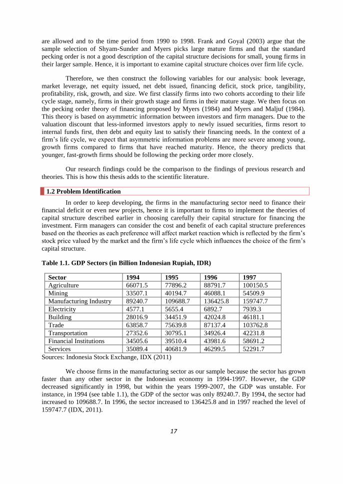
1.2 Problem Identification
In order to keep developing, the firms in the manufacturing sector need to finance their
financial deficit or even new projects, hence it is important to firms to implement the theories of
capital structure described earlier in choosing carefully their capital structure for financing the
investment. Firm managers can consider the cost and benefit of each capital structure preferences
based on the theories as each preference will affect market reaction which is reflected by the firm‟s
stock price valued by the market and the firm‟s life cycle which influences the choice of the firm‟s
capital structure.
Table 1.1. GDP Sectors (in Billion Indonesian Rupiah, IDR)
Sector 1994 1995 1996 1997
Agriculture 66071.5 77896.2 88791.7 100150.5
Mining 33507.1 40194.7 46088.1 54509.9
Manufacturing Industry 89240.7 109688.7 136425.8 159747.7
Electricity 4577.1 5655.4 6892.7 7939.3
Building 28016.9 34451.9 42024.8 46181.1
Trade 63858.7 75639.8 87137.4 103762.8
Transportation 27352.6 30795.1 34926.4 42231.8
Financial Institutions 34505.6 39510.4 43981.6 58691.2
Services 35089.4 40681.9 46299.5 52291.7
Sources: Indonesia Stock Exchange, IDX (2011)
We choose firms in the manufacturing sector as our sample because the sector has grown
faster than any other sector in the Indonesian economy in 1994-1997. However, the GDP
decreased significantly in 1998, but within the years 1999-2007, the GDP was unstable. For
instance, in 1994 (see table 1.1), the GDP of the sector was only 89240.7. By 1994, the sector had
increased to 109688.7. In 1996, the sector increased to 136425.8 and in 1997 reached the level of
159747.7 (IDX, 2011).
18
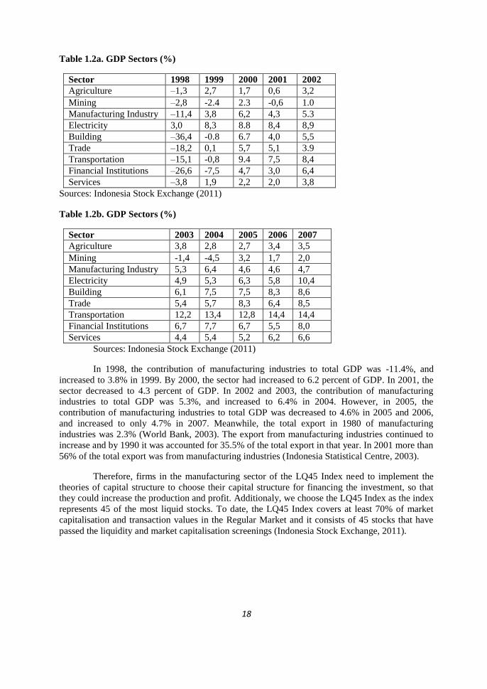
Table 1.2a. GDP Sectors (%)
Sector 1998 1999 2000 2001 2002
Agriculture –1,3 2,7 1,7 0,6 3,2
Mining –2,8 -2.4 2.3 -0,6 1.0
Manufacturing Industry –11,4 3,8 6,2 4,3 5.3
Electricity 3,0 8,3 8.8 8,4 8,9
Building –36,4 -0.8 6.7 4,0 5,5
Trade –18,2 0,1 5,7 5,1 3.9
Transportation –15,1 -0,8 9.4 7,5 8,4
Financial Institutions –26,6 -7,5 4,7 3,0 6,4
Services –3,8 1,9 2,2 2,0 3,8
Sources: Indonesia Stock Exchange (2011)
Table 1.2b. GDP Sectors (%)
Sector 2003 2004 2005 2006 2007
Agriculture 3,8 2,8 2,7 3,4 3,5
Mining -1,4 -4,5 3,2 1,7 2,0
Manufacturing Industry 5,3 6,4 4,6 4,6 4,7
Electricity 4,9 5,3 6,3 5,8 10,4
Building 6,1 7,5 7,5 8,3 8,6
Trade 5,4 5,7 8,3 6,4 8,5
Transportation 12,2 13,4 12,8 14,4 14,4
Financial Institutions 6,7 7,7 6,7 5,5 8,0
Services 4,4 5,4 5,2 6,2 6,6
Sources: Indonesia Stock Exchange (2011)
In 1998, the contribution of manufacturing industries to total GDP was -11.4%, and
increased to 3.8% in 1999. By 2000, the sector had increased to 6.2 percent of GDP. In 2001, the
sector decreased to 4.3 percent of GDP. In 2002 and 2003, the contribution of manufacturing
industries to total GDP was 5.3%, and increased to 6.4% in 2004. However, in 2005, the
contribution of manufacturing industries to total GDP was decreased to 4.6% in 2005 and 2006,
and increased to only 4.7% in 2007. Meanwhile, the total export in 1980 of manufacturing
industries was 2.3% (World Bank, 2003). The export from manufacturing industries continued to
increase and by 1990 it was accounted for 35.5% of the total export in that year. In 2001 more than
56% of the total export was from manufacturing industries (Indonesia Statistical Centre, 2003).
Therefore, firms in the manufacturing sector of the LQ45 Index need to implement the
theories of capital structure to choose their capital structure for financing the investment, so that
they could increase the production and profit. Additionaly, we choose the LQ45 Index as the index
represents 45 of the most liquid stocks. To date, the LQ45 Index covers at least 70% of market
capitalisation and transaction values in the Regular Market and it consists of 45 stocks that have
passed the liquidity and market capitalisation screenings (Indonesia Stock Exchange, 2011).

19
1.3 Research Questions
The research is going to answer the following major and minor research questions:
1.3.1 Major Research Questions
Our major research questions are as follow:
1. What are the determinants of capital structure of the firms in the manufacturing sector in
Indonesia?
2. How do firms in the manufacturing sector in Indonesia raise capital for investments,
internally or externally (with debt, equity, or debt to repurchase equity)?
3. Does debt policy matter?
4. In the context of firm‟s life cycle, can we expect that growth [and small] firms follow the
pecking order theory more closely than mature [and large] firms?
1.3.2 Minor Research Questions
Our minor research questions are as follow:
1. What are the determinants of capital structure of the firms in the manufacturing sector in
Indonesia?
a. As implied by the trade-off theory and the pecking order theory, do growth
opportunities have a positive relationship with the debt ratio?
b. As in the pecking order hypothesis, does the firm‟s profitability have a negative
relationship with the level of debt? And as implied by the trade-off theory, does the
firm‟s profitability have a positive relationship with the debt ratio?
c. In accordance with the pecking order theory and trade-off theory, is there a negative
relationship between risk (earnings volatility) and debt ratio?
d. As suggested by the trade-off theory, does size have a positive relationship with the
debt ratio? And as suggested by the pecking order theory of the capital structure, is
there a negative relationship between the level of debt and the size of the firm?
e. In accordance with the trade-off theory, is there a positive relationship between the
asset tangibility and the level of debt?
2. How do firms in the manufacturing sector in Indonesia raise capital for investments,
internally or externally (with debt, equity, or debt to repurchase equity)?
3. Does debt policy matter?
Based on the asymmetric information, the firms use equity financing only as the last
resort and based on signalling theory, the markets normally react favourably to moderate
increases in leverage and negatively to a fresh issue of equity.
20
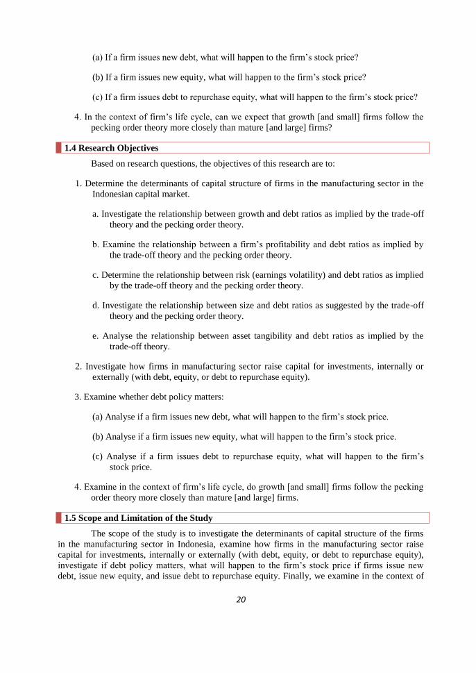
(a) If a firm issues new debt, what will happen to the firm‟s stock price?
(b) If a firm issues new equity, what will happen to the firm‟s stock price?
(c) If a firm issues debt to repurchase equity, what will happen to the firm‟s stock price?
4. In the context of firm‟s life cycle, can we expect that growth [and small] firms follow the
pecking order theory more closely than mature [and large] firms?
1.4 Research Objectives
Based on research questions, the objectives of this research are to:
1. Determine the determinants of capital structure of firms in the manufacturing sector in the
Indonesian capital market.
a. Investigate the relationship between growth and debt ratios as implied by the trade-off
theory and the pecking order theory.
b. Examine the relationship between a firm‟s profitability and debt ratios as implied by
the trade-off theory and the pecking order theory.
c. Determine the relationship between risk (earnings volatility) and debt ratios as implied
by the trade-off theory and the pecking order theory.
d. Investigate the relationship between size and debt ratios as suggested by the trade-off
theory and the pecking order theory.
e. Analyse the relationship between asset tangibility and debt ratios as implied by the
trade-off theory.
2. Investigate how firms in manufacturing sector raise capital for investments, internally or
externally (with debt, equity, or debt to repurchase equity).
3. Examine whether debt policy matters:
(a) Analyse if a firm issues new debt, what will happen to the firm‟s stock price.
(b) Analyse if a firm issues new equity, what will happen to the firm‟s stock price.
(c) Analyse if a firm issues debt to repurchase equity, what will happen to the firm‟s
stock price.
4. Examine in the context of firm‟s life cycle, do growth [and small] firms follow the pecking
order theory more closely than mature [and large] firms.
1.5 Scope and Limitation of the Study
The scope of the study is to investigate the determinants of capital structure of the firms
in the manufacturing sector in Indonesia, examine how firms in the manufacturing sector raise
capital for investments, internally or externally (with debt, equity, or debt to repurchase equity),
investigate if debt policy matters, what will happen to the firm‟s stock price if firms issue new
debt, issue new equity, and issue debt to repurchase equity. Finally, we examine in the context of

21
firm‟s life cycle, do growth [and small] firms follow the pecking order theory more closely than
mature [and large] firms.
Manufacturing companies that exist throughout the 13-year period with no missing data
are included in the study. Data availability is a major limitation in capital structure studies in
emerging capital markets. We use data of the Indonesia Stock Exchange Main Board companies,
with the selected time period of 1994-2007 to capture the differences in economic conditions of
the Indonesian economy. To enlighten it, we explain those periods that describe the differences in
economic conditions.
Before the Crisis Period (Before 1997)
Before the economic crisis triggered by the financial crisis in mid 1997, Indonesia was
among the few developing countries which were rated as highly successful in its development.
Within thirty years, from 1965 to 1995, GDP per capita in real terms grew on average by 6.6%
annually (World Bank 1997). The role of manufacturing industry in GDP experienced a significant
increased, from 7.6% in 1973 to nearly 25% in 1995.
Crisis Period (1997-1998)
In 1995 Indonesia was still enjoying an economic growth of 8.2%, later in 1996, or the
last year before the crisis happened, it still grew with 7.8%, and in 1997 dropped to 4.9%. So, until
1997, the year of the crisis, at least, economic growth still remained positive despite showing a
declining trend. The crisis that began with the fall of the Thai Baht in July 1997, then gave a direct
result on the value of IDR which depreciated exponentially, from Rp2.400 per Dollar in mid-1997
to Rp16.000 per Dollar in June 1998. The decline in food production triggered high inflation in
1998, added pressuring on foreign exchange reserves that have already declined.
In 1998, when the crisis reached its peak, Indonesia's economic growth contracted by
13.6% and other macroeconomic indicators showed worsening values, such as inflation which
increased to 77.6%. The crisis that hit Indonesia since mid 1997 has gradually decreased and by
the end of the reporting year 1998/99 Indonesian economy began to show improvement.
Inflationary pressures continued to decline from October 1998 onwards, so that the annual
inflation rate had reached 82.4% in September 1998, and was successfully reduced to 45.4% at the
year-end report. The success in reducing inflationary pressures reflected in the strengthening trend
of the IDR.
1999-2000
In 1999, inflation rate was under control, from almost 80% in 1998 to 2% in the
following year, With these conditions, the interest rate could drop from about 80% to 11-12%. By
mid-1999, the economic crisis in Indonesia had surpassed its lowest point and began to grow
again. Throughout the year, the economy grew slightly with an increase in GDP of 0.3%.
Entering early 2000, the process of economic recovery had begun to appear since the
third quarter of 1999. Monetary stability was also controllable, as reflected in the achievement of
low inflation and stronger exchange rate until the end of 1999. Economic growth was increasing
higher than forecasted to 4.8%. The IDR tended to weaken and volatile since May 2000.
Meanwhile, pressure on the inflation rate increased and inflationary pressures also emerged as a
result of the weakening of the IDR.
22
2001-2004
During the 2001, economic and monetary conditions in general showed a deteriorating
trend. Worsening the economic and monetary conditions, among others, indicated by the slowing
economic growth, a weakening exchange rate, and high inflation pressures. During 2001,
Indonesia's economy grew only by 3.3%, the exchange rate depreciated by 17.7% so that to
achieve an average of Rp.10.255 per USD Dollar, and CPI inflation reached 12.55%.
During 2002, the general economic condition in Indonesia showed a positive growth
which was indicated by more stable macroeconomic conditions. Overall, in 2002, the exchange
rate appreciated significantly by 10.10% so as to achieve an average of Rp 9.316 per US Dollar.
These stable monetary conditions have affected the level of CPI inflation during 2002,
experiencing a declining trend to reach 10.03%. Overall, during 2002 the Indonesian economy
only grew by 3.7%.
In 2003, to face the challenges, the Government and the Bank of Indonesia have taken a
series of policies to encourage the process of economic recovery while maintaining
macroeconomic stability. In the process, various policies have contributed significantly in
supporting the achievement of stable macro economic conditions during 2003, which indicated by
the strengthening of the IDR and declining of inflation rate. The year 2004 brang hope, optimism,
as well as a new challenge. In 2004, macroeconomic stability maintained, international confidence
increased, and clarity of the economic agenda eached.
2005-2007
The year 2005 was a dynamic and challenging one for the economy of Indonesia. On the
average, the Rupiah reached Rp 9.713 per U.S. Dollar during 2005, or a depreciation by 8.6%
compared to an average of 2004. Meanwhile, the CPI inflation, which until the third quarter of
2005 was recorded at 9.1% (year on year, yoy) had increased to 17.1% (yoy) in late 2005. Overall
economic growth in Indonesia in 2005 reached 5.6% or achieved an increase of 5.1% from the
previous year.
Entering the beginning of 2006, Indonesia economic conditions are still very influenced
by the rising of fuel prices (fuel) and high interest rates. Inflation rate of consumer price index
(CPI) which is very high in early 2006 reached 17.03% (yoy) gradually decreased to 6.60% (yoy)
in late 2006 and maintained stability in the rupiah. With inflation and interest rates which
gradually declined, since the beginning of the second half of 2006, the economy grew in the good
trend so as the overall in 2006, growth reached 5.5% (yoy), slightly lower than the previous year.
Entering 2007, Indonesia's economy to regain macroeconomic stability. The Rupiah, in
the second half of 2007 was depreciated significantly and reached the weakest level in August
2007, with a monthly average of Rp 9372 per U.S. Dollar. Maintained macroeconomic stability
kept a high economic growth in 2007, and even reached the highest level in the post-crisis period,
namely 6.32%.
1.6 Expected Contribution
By conducting this research, we expected some contributions for the firms. In this research, the
purpose of our research will not be to produce a theory that is generalisable to all populations. Our
objective is trying to explain what is happening in the Indonesian capital market with
manufacturing firms of the LQ45 Index, regarding how firms finance their operations. What
factors influence the choices of capital structure? How do these choices affect the stock price? And
23
how do firms finance their deficit over a firm‟s life cycle? The findings of this study will lead
firms to make the decision of choosing capital structure by considering the firm‟s characteristics,
market reaction reflected by stock price, and the life cycle stage of the firm.
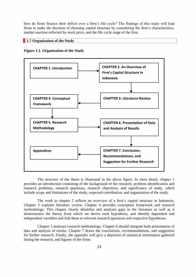
1.7 Organisation of the Study
Figure 1.1. Organisation of the Study
The structure of the thesis is illustrated in the above figure. In more detail, chapter 1
provides an introduction consisting of the background of the research, problem identification and
research problems, research questions, research objectives, and significance of study, which
include scope and limitations of the study, expected contribution, and organisation of the study.
The work in chapter 2 reflects an overview of a firm‟s capital structure in Indonesia.
Chapter 3 explains literature review. Chapter 4 provides conceptual framework and research
methodology. This chapter clearly identifies and analyses gaps in the literature as well as it
demonstrates the theory from which we derive each hypothesis, and identify dependent and
independent variables and link these to relevant research questions and respective hypotheses.
Chapter 5 analyses research methodology. Chapter 6 should integrate both presentation of
data and analysis of results. Chapter 7 draws the conclusions, recommendations, and suggestion
for further research. Finally, the appendix will give a depiction of statistical information gathered
during the research, and figures of the firms.
CHAPTER 1. Introduction CHAPTER 2. An Overview of
Firm’s Capital Structure in
Indonesia
CHAPTER 3. Literature Review CHAPTER 4. Conceptual
Framework
CHAPTER 6. Presentation of Data
and Analysis of Results
CHAPTER 7. Conclusion,
Recommendations, and
Suggestion for Further Research
Appendices
CHAPTER 5. Research
Methodology

24
2. AN OVERVIEW OF THE CAPITAL STRUCTURE OF INDONESIAN
MANUFACTURING FIRMS
2.1. Indonesian Capital Market
The capital market plays an important role in the economy of a country, including
Indonesia, because it serves two functions at the same time. First, the capital market serves as an
alternative for a company's capital resources. The capital gained from the public offering can be
used for the company's business development, expansion, and so on. Second, the capital market
serves as an alternative for public investment. People could invest their money according to their
preferred returns and risk characteristics of each instrument.
2.1.1 History of Indonesia Stock Exchange
Below is the brief history of the Indonesia Stock Exchange. The first Stock Exchange in
Indonesia was built in Batavia (currently known as Jakarta) in December 1912. The Batavia Stock
Exchange was closed during the years 1914 -1918. It was re-opened in 1925 and new stock
exchanges were established in Semarang and Surabaya. However, between 1919 and 1924, the
Indonesia Stock Exchange (IDX) was still closed.
The Jakarta Stock Exchange (JSX) was re-closed during the years 1942 – 1952. On
August 10, 1977, the Exchange was re-activated by President Soeharto. It was supervised under
the management of the Capital Market Supervisory Agency (Badan Pengawas Pasar Modal, or
BAPEPAM). The re-activation of the capital market was also marked by the going public of PT
Semen Cibinong as the first issuer listed in the JSX. July 10th is celebrated as the anniversary of
the Capital Market in Indonesia.
In 1977 – 1987, the activity of stock trading in the JSX was dull. There were only 24
listed companies in the JSX. Most people preferred to invest their money in banks rather than the
capital market. December Package 1987) was issued to give ways for companies to go public and
for foreign investors to invest their money in Indonesia in 1987. In 1988 – 1990, deregulation
packages in banking and capital market were made. The JSX welcomed foreign investors. The
activities of the JSX were improving. On June 16, 1989, the Surabaya Stock Exchange started to
operate and was managed by the Surabaya Stock Exchange Inc.
On July 13, 1992, the JSX was privatised, and this date is celebrated as the anniversary of
the Jakarta Stock Exchange. The JSX introduced its computerized Jakarta Automatic Trading
System (JATS) on May 22, 1995. On November 10, 1995, the Government of Indonesia issued
Regulations No. 8 year 1995 on the capital market. This regulation was effective from January
1996. The JSX started to implement the remote trading system in 2002. In 2007, the Surabaya
Stock Exchange was merged into Jakarta Stock Exchange. As a result, the JSX changed its name
into the Indonesia Stock Exchange.
2.1.2 Stock Price Index in the Indonesian Capital Market
In order to give more complete information on the stock exchange development to the
public, the Indonesian Stock Exchange (IDX) has spread the indicators of the stock price

25
movement through the printed and electronic media. One indicator of the stock price movement is
the Stock Price Index. At present, the JSX has 9 constituent Stock Price Indices and 10 sectors:
Composite Stock Price Index (CSPI), Main Board Index (MBX), Kompas 100, Liquid 45
(LQ45), Jakarta Islamic Index, Development Board Index (DBX), Indonesian Securties Rating
Agency (PEFINDO25), BISNIS-27, and Sustainable Responsible Investment-Indonesian
Biodiversity Foundation. The sectors include mining, agriculture, consumers, miscellaneous-
industry, manufacture, infrastructure, finance, trade, basic-industry, and property.
The following indices are guidelines for investors to make stock investment in the
Indonesian capital market.
1. The Composite Stock Price Index (CSPI), the index that uses all of the Companies Listed as a
component of index calculation. The Composite Stock Price Index (CSPI) was introduced the
first time on April 1st, 1983 as an indicator of the movement of all listed stock prices in the
JSX, for both the regular and the preferred stocks. The base day for the CSPI‟s calculation is
on August 10th
, 1982. At that date, the index was determined at 100, and the listed number of
stocks at that time was thirteen.
2. The JSX LQ45 Index was created to provide the market with an index that represents 45 of
the most liquid stocks. To date, the LQ45 Index covers at least 70% of the market
capitalisation and transaction values in the Regular Market. The LQ45 Index of historical
calculation was defined on July 13, 1994, with a base value of 100. The index consists of 45
stocks that have passed the liquidity and market capitalisation screenings.
3. The Jakarta Islamic Index was launched on July 3, 2000. The index consists of 30 stocks that
have passed the selection under the direction of the Sharia Supervisory Board of the Majelis
Ulama Indonesia. Stocks from listed companies with business activities that comply with the
Islamic sharia can be included into the index.
4. The Kompas 100 Index is an index consisting of 100 shares of Listed Companies that are
selected, based on considerations of liquidity and market capitalisation, in line with
predetermined criteria.
5. The Index BUSINESS-27 is a collaboration between the IDX and Bisnis Indonesia Daily. The
Stock index Listed Companies are selected based on fundamental criteria, technical or
liquidity of transactions and accountability and corporate governance.
6. The PEFINDO-25 Index is a collaboration between the BEI and the PEFINDO rating
agencies, which is intended to provide additional information for investors, especially for the
shares of small and medium-sized listed companies (Small Medium Enterprises/SME).
7. The Sustainable Responsible Investment-KEHATI Index is the index established for
cooperation between the BEI and the Indonesian Biodiversity Foundation (KEHATI). This
index is expected to provide additional information to investors who want to invest in stocks
that have excellent performance in encouraging sustainable business, and have awareness of
the environment and run good corporate governance.
8. The Main Board Index (MBX) and the Development Board Index (DBX). On July13th
, 2000,
the JSX launched a new rule on stock listing: the Two Board Listing System. This system is
implemented to stimulate the Indonesian Capital Market and also to recover public confidence
for the Exchange through the arrangement of good corporate governance.
9. Sectoral indices, the index that uses all the Listed Companies included in each sector. Today
there are 10 sectors in the IDX, namely agriculture; mining;, primary industrie;, miscellaneous
industry;, consumer goods; property; infrastructure; finance; trade and services; and
manufacture.

26
2.1.3. Description of the LQ45 Index
We chose the LQ45 Index as our population as LQ45 Index consists of 45 stocks with
high liquidity. The Indonesia Stock Exchange regularly monitors the performance progress of the
stock components which are included in the calculation of the LQ45 index. Every three months an
evaluation on the movement sequence of the shares is conducted. Replacement shares will be
conducted every six months, i.e. at the beginning of February and August. Therefore, we chose the
LQ45 index as our population in this research.
Since its launch in February 1997, the primary measure of liquidity transaction is the
value of transactions in the regular market. In accordance with market developments, and to
sharpen further the criteria of liquidity, since the review in January 2005, the number of trading
days and the frequency of transactions has been included as a measure of liquidity. Thus, the
criterium of stock that is to be included in the calculation of the LQ45 Index is as follows:
1. Has been listed on the Stock Exchange at least 3 months
2. Log in 60 stocks based on the value of transactions in the regular market
3. Of the 60 stocks, 30 stocks with the largest transaction value will automatically be included on
the calculation of the index LQ45.
4. To get 45 shares 15 shares will be selected again by using the criteria of day transaction in
regular market, frequency of transaction in regular market and market capitalisation. 15 stocks
selection methods are the following:
a. 30 of the remaining stocks, 25 stocks are selected based on transactions day in the regular
market.
b. 25 of the stocks 20 stocks will be selected based on the frequency of transactions in the
regular market.
c. 20 of the stocks will be selected 15 stocks based on market capitalisation, so it will get 45
shares for calculation of the LQ45 Index.
5. In addition to considering the liquidity criteria and market capitalisation mentioned above, will
be seen also the financial condition and prospects of the company's growth.
2.2. Characteristics of the Research Sample
We constructed two samples of firms according to their life cycle stage, namely, firms in
their growth stage and firms in their mature stage. Bulan and Yan (2009) defined the growth stage
as the first six-year-period after the year of the firm‟s initial public offering (IPO). They treated the
IPO as the starting point of the growth stage (or the “new growth” stage). Hence, we follow them
to identify the growth stage. We took Grullon, Michaely and Swaminathan (2000), DeAngelo,
DeAngelo and Stulz (2005) and Bulan, Subramanian and Tanlu as the references (2007) who
found that firms initiated dividends were mature firms. Thus, we identified firms in their mature
stage by their dividend history.
Meanwhile, we defined six years old or younger as young firms and seven years or older
as old firms. We followed Bulan and Yan (2007) and Evans (1987) to set the length of each stage
to be 6 years. Finally, we defined "small" as firms with total assets of less than $150 million, and
large firms that have total asset of more than $150 millions (Hufft, JR), it equals to IDR
1,081,028.68 or 1,086,876.61.
27
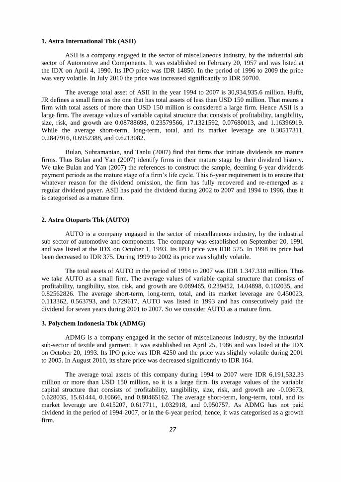
1. Astra International Tbk (ASII)
ASII is a company engaged in the sector of miscellaneous industry, by the industrial sub
sector of Automotive and Components. It was established on February 20, 1957 and was listed at
the IDX on April 4, 1990. Its IPO price was IDR 14850. In the period of 1996 to 2009 the price
was very volatile. In July 2010 the price was increased significantly to IDR 50700.
The average total asset of ASII in the year 1994 to 2007 is 30,934,935.6 million. Hufft,
JR defines a small firm as the one that has total assets of less than USD 150 million. That means a
firm with total assets of more than USD 150 million is considered a large firm. Hence ASII is a
large firm. The average values of variable capital structure that consists of profitability, tangibility,
size, risk, and growth are 0.08788698, 0.23579566, 17.1321592, 0.07680013, and 1.16396919.
While the average short-term, long-term, total, and its market leverage are 0.30517311,
0.2847916, 0.6952388, and 0.6213082.
Bulan, Subramanian, and Tanlu (2007) find that firms that initiate dividends are mature
firms. Thus Bulan and Yan (2007) identify firms in their mature stage by their dividend history.
We take Bulan and Yan (2007) the references to construct the sample, deeming 6-year dividends
payment periods as the mature stage of a firm‟s life cycle. This 6-year requirement is to ensure that
whatever reason for the dividend omission, the firm has fully recovered and re-emerged as a
regular dividend payer. ASII has paid the dividend during 2002 to 2007 and 1994 to 1996, thus it
is categorised as a mature firm.
2. Astra Otoparts Tbk (AUTO)
AUTO is a company engaged in the sector of miscellaneous industry, by the industrial
sub-sector of automotive and components. The company was established on September 20, 1991
and was listed at the IDX on October 1, 1993. Its IPO price was IDR 575. In 1998 its price had
been decreased to IDR 375. During 1999 to 2002 its price was slightly volatile.
The total assets of AUTO in the period of 1994 to 2007 was IDR 1.347.318 million. Thus
we take AUTO as a small firm. The average values of variable capital structure that consists of
profitability, tangibility, size, risk, and growth are 0.089465, 0.239452, 14.04898, 0.102035, and
0.82562826. The average short-term, long-term, total, and its market leverage are 0.450023,
0.113362, 0.563793, and 0.729617, AUTO was listed in 1993 and has consecutively paid the
dividend for seven years during 2001 to 2007. So we consider AUTO as a mature firm.
3. Polychem Indonesia Tbk (ADMG)
ADMG is a company engaged in the sector of miscellaneous industry, by the industrial
sub-sector of textile and garment. It was established on April 25, 1986 and was listed at the IDX
on October 20, 1993. Its IPO price was IDR 4250 and the price was slightly volatile during 2001
to 2005. In August 2010, its share price was decreased significantly to IDR 164.
The average total assets of this company during 1994 to 2007 were IDR 6,191,532.33
million or more than USD 150 million, so it is a large firm. Its average values of the variable
capital structure that consists of profitability, tangibility, size, risk, and growth are -0.03673,
0.628035, 15.61444, 0.10666, and 0.80465162. The average short-term, long-term, total, and its
market leverage are 0.415207, 0.617711, 1.032918, and 0.950757. As ADMG has not paid
dividend in the period of 1994-2007, or in the 6-year period, hence, it was categorised as a growth
firm.

28
4. Barito Pacific Tbk (BRPT)
BRPT is a company engaged in the sector of basic industry and chemicals, by the
industrial sub-sector of chemicals. It was established on April 4, 1979 and was listed at the IDX on
October 1, 1993. Its IPO price was IDR 7200 and the price was very volatile during 1996 to 2007.
In 2001 it hit the lowest price of IDR 50, but in July 2010, it bounced to IDR 1060. But still it is
lower than its IPO price.
We take BRPT as a large firm since the average total assets during 1994 to 2007 were
IDR 4,107,897.43 million or over USD 150 million. The average values of variable capital
structure that consists of profitability, tangibility, size, risk, and growth are -0.01767, 0.147128,
15.121, 0.0757, and 1.5739773. The average short-term, long-term, total, and its market leverage
are 0.4942, 0.179966, 0.673681, and 0.750922. BRPT has paid dividend to shareholders in 1994-
1996, thus, it is categorised as a growth firm.
5. Budi Acid Jaya Tbk (BUDI)
BUDI is a company engaged in the sector of basic industry and chemicals, by the
industrial sub-sector of chemicals. It was established in Jan 15, 1979 and was listed at the IDX on
May 8, 1995. Its IPO price was IDR 3000 and the price during 199 to 2000 was very volatile. In
August 2010 it was decreased significantly to IDR 335.
We take this company as small firm since its average total assets in 1994 to 2007 were
IDR 496,726.67 million or less than USD 150 million. Its average values of variable capital
structure that consists of profitability, tangibility, size, risk, and growth, are 0.095584, 0.504481,
12.89337, 0.092448, and 0.72631332. The average short-term, long-term, total, and its market
leverage are 0.283404, 0.344108, 0.571919, and 0.812384. BUDI has paid dividend in 1994 to
1996, 1999, and 2006 to 2007, but it was not paid in the six year period consecutively thus, it is
categorised as a growth firm.
6. Charoen Pokphand Indonesia Tbk (CPIN)
CPIN is a company engaged in the sector of basic industry and chemicals, by the
industrial sub-sector of pet food. It was established on January 7, 1973 and was listed at the IDX
on March 18, 1991. The IPO price was IDR 5100 and the price was quite volatile in 1996 to 2000
and in 2003 to 2007. But in August 2010, it was increased to IDR 6450 million, or more than USD
150 million. Its average values of variable capital structure that consists of profitability, tangibility,
size, risk, and growth, are 0.048659, 0.30468, 14.31341, 0.080364, and 1.25243854. CPIN is a
growing firm since it paid the dividend not in 6 consecutive years in 1994 to 1996, and 2006.
7. Dankos Laboratories Tbk (DNKS)
DNKS is a company engaged in the sector of pharmaceuticals. It was established on
March 25, 1974 and was listed at the IDX on November 13, 1989. The IPO price was IDR 6500.
The price was quite volatile in 1996 to 2002 and hit the lowest price of IDR 250.
DNKS is a small firm since its average total assets in 1994 to 2007 was IDR 377,072.67
million or less than USD 150 million. Its average values of variable capital structure that consists
of profitability, tangibility, size, risk, and growth, are 0.108408, 0.136731, 12.72363, 0.095927,
and 0.96989997. The average short-term, long-term, total, and its market leverage are 0.36937,
0.27362, 0.584694, and 0.724032. DNKS is a growing firm since it did not pay the dividend in 6
consecutive years.
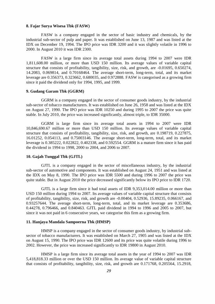
29
8. Fajar Surya Wisesa Tbk (FASW)
FASW is a company engaged in the sector of basic industry and chemicals, by the
industrial sub-sector of pulp and paper. It was established on June 13, 1987 and was listed at the
IDX on December 19, 1994. The IPO price was IDR 3200 and it was slightly volatile in 1996 to
2000. In August 2010 it was IDR 2300.
FASW is a large firm since its average total assets during 1994 to 2007 were IDR
1,811,608.00 million, or more than USD 150 million. Its average values of variable capital
structure that consists of profitability, tangibility, size, risk, and growth, are -0.01695, 0.650274,
14.2083, 0.069814, and 0.70168464. The average short-term, long-term, total, and its market
leverage are 0.356373, 0.323662, 0.680035, and 0.972888. FASW is categorised as a growing firm
since it paid the dividend only for 1994, 1995, and 1999.
9. Gudang Garam Tbk (GGRM)
GGRM is a company engaged in the sector of consumer goods industry, by the industrial
sub-sector of tobacco manufacturers. It was established on June 26, 1958 and was listed at the IDX
on August 27, 1990. The IPO price was IDR 10250 and during 1995 to 2007 the price was quite
stable. In July 2010, the price was increased significantly, almost triple, to IDR 35000.
GGRM is large firm since its average total assets in 1994 to 2007 were IDR
10,846,690.67 million or more than USD 150 million. Its average values of variable capital
structure that consists of profitability, tangibility, size, risk, and growth, are 0.198719, 0.227875,
16.01252, 0.054113, and 0.75003146. The average short-term, long-term, total, and its market
leverage is 0.385222, 0.022822, 0.402338, and 0.592554. GGRM is a mature firm since it has paid
the dividend in 1994 to 1998, 2000 to 2004, and 2006 to 2007.
10. Gajah Tunggal Tbk (GJTL)
GJTL is a company engaged in the sector of miscellaneous industry, by the industrial
sub-sector of automotive and components. It was established on August 24, 1951 and was listed at
the IDX on May 8, 1990. The IPO price was IDR 5500 and during 1996 to 2007 the price was
quite stable. But in August 2010 the price decreased significantly below its IPO price to IDR 1720.
GJTL is a large firm since it had total assets of IDR 9,353,014.00 million or more than
USD 150 million during 1994 to 2007. Its average values of variable capital structure that consists
of profitability, tangibility, size, risk, and growth are -0.00404, 0.52936, 15.89235, 0.066167, and
0.93257644. The average short-term, long-term, total, and its market leverage are 0.353686,
0.44278, 0.796466, and 0.840463. GJTL paid dividend in 1994 to 1996 and 2005 to 2007, but
since it was not paid in 6 consecutive years, we categorise this firm as a growing firm.
11. Hanjaya Mandala Sampoerna Tbk (HMSP)
HMSP is a company engaged in the sector of consumer goods industry, by industrial sub-
sector of tobacco manufacturers. It was established on March 27, 1905 and was listed at the IDX
on August 15, 1990. The IPO price was IDR 12600 and its price was quite volatile during 1996 to
2002. However, the price was increased significantly to IDR 19800 in August 2010.
HMSP is a large firm since its average total assets in the year of 1994 to 2007 was IDR
5,418,818.33 million or over the USD 150 million. Its average value of variable capital structure
that consists of profitability, tangibility, size, risk, and growth are 0.171768, 0.205564, 15.2918,
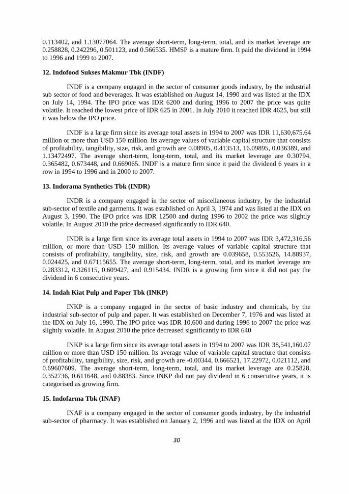
30
0.113402, and 1.13077064. The average short-term, long-term, total, and its market leverage are
0.258828, 0.242296, 0.501123, and 0.566535. HMSP is a mature firm. It paid the dividend in 1994
to 1996 and 1999 to 2007.
12. Indofood Sukses Makmur Tbk (INDF)
INDF is a company engaged in the sector of consumer goods industry, by the industrial
sub sector of food and beverages. It was established on August 14, 1990 and was listed at the IDX
on July 14, 1994. The IPO price was IDR 6200 and during 1996 to 2007 the price was quite
volatile. It reached the lowest price of IDR 625 in 2001. In July 2010 it reached IDR 4625, but still
it was below the IPO price.
INDF is a large firm since its average total assets in 1994 to 2007 was IDR 11,630,675.64
million or more than USD 150 million. Its average values of variable capital structure that consists
of profitability, tangibility, size, risk, and growth are 0.08905, 0.413513, 16.09895, 0.036389, and
1.13472497. The average short-term, long-term, total, and its market leverage are 0.30794,
0.365482, 0.673448, and 0.669065. INDF is a mature firm since it paid the dividend 6 years in a
row in 1994 to 1996 and in 2000 to 2007.
13. Indorama Synthetics Tbk (INDR)
INDR is a company engaged in the sector of miscellaneous industry, by the industrial
sub-sector of textile and garments. It was established on April 3, 1974 and was listed at the IDX on
August 3, 1990. The IPO price was IDR 12500 and during 1996 to 2002 the price was slightly
volatile. In August 2010 the price decreased significantly to IDR 640.
INDR is a large firm since its average total assets in 1994 to 2007 was IDR 3,472,316.56
million, or more than USD 150 million. Its average values of variable capital structure that
consists of profitability, tangibility, size, risk, and growth are 0.039658, 0.553526, 14.88937,
0.024425, and 0.67115655. The average short-term, long-term, total, and its market leverage are
0.283312, 0.326115, 0.609427, and 0.915434. INDR is a growing firm since it did not pay the
dividend in 6 consecutive years.
14. Indah Kiat Pulp and Paper Tbk (INKP)
INKP is a company engaged in the sector of basic industry and chemicals, by the
industrial sub-sector of pulp and paper. It was established on December 7, 1976 and was listed at
the IDX on July 16, 1990. The IPO price was IDR 10,600 and during 1996 to 2007 the price was
slightly volatile. In August 2010 the price decreased significantly to IDR 640
INKP is a large firm since its average total assets in 1994 to 2007 was IDR 38,541,160.07
million or more than USD 150 million. Its average value of variable capital structure that consists
of profitability, tangibility, size, risk, and growth are -0.00344, 0.666521, 17.22972, 0.021112, and
0.69607609. The average short-term, long-term, total, and its market leverage are 0.25828,
0.352736, 0.611648, and 0.88383. Since INKP did not pay dividend in 6 consecutive years, it is
categorised as growing firm.
15. Indofarma Tbk (INAF)
INAF is a company engaged in the sector of consumer goods industry, by the industrial
sub-sector of pharmacy. It was established on January 2, 1996 and was listed at the IDX on April
31
17, 2001. The IPO price was IDR 250 and it was quite stable from 2001 to 2002 and from 2006 to
2007.
INAF is a small firm since its average total assets in 1994 to 2007 was IDR 549,373.33
million or less than USD 150 million. Its average values of variable capital structure that consists
of profitability, tangibility, size, risk, and growth are 0.191893, 0.161847, 13.08003, 0.106093,
and 0.6048993. The average short-term, long-term, total, and its market leverage are 0.385286,
0.088814, 0.429693, and 0.810453. INAF has paid dividend in 2000-2001, thus we decide to
categorise it as a growth firm.
16. Indocement Tunggal Prakasa Tbk (INTP)
INTP is a company engaged in the sector of basic industry and chemicals, by the
industrial sub sector of cement. It was established on January 16, 1985 and was listed at the IDX
on December 5, 1989. The IPO price was IDR 10,000 and during 1998 to 2007 the price was quite
volatile. In July 2010 the price increased significantly to IDR 16900.
INTP is a large firm since its average total assets in 1994 to 2007 was IDR 6,510,362.43
million or more than USD 150 million. Its average values of variable capital structure that consists
of profitability, tangibility, size, risk, and growth are 0.006746, 0.749494, 16.11841, 0.081079,
and 0.86040421. The average short-term, long-term, total, and its market leverage are 0.265209,
0.456302, 0.721511, and 0.839875. INTP has paid dividend in 2005-2007, thus we decide to
categorise it as a growth firm.
17. Kalbe Farma Tbk (KLBF)
KLBF is a company engaged in the sector of consumer goods industry, by the industrial
sub sector of pharmacy. It was established on September 10, 1966 and was listed at the IDX on
July 30, 1991. Its IPO price was IDR 7800 and it was slightly volatile in 1996 to 2007. In July
2010 the price decreased significantly to IDR 2450.
KLBF is a large firm since its average total assets in 1994 to 2007 was IDR 2,564,165.14
million or more than USD 150 million. Its average values of variable capital structure that consists
of profitability, tangibility, size, risk, and growth are 0.112514, 0.17985, 14.63738, 0.08441, and
1.22087525. The average short-term, long-term, total, and its market leverage are 0.112514,
0.17985, 14.63738, 0.08441, and 1.22087525. KLBF is categorised as a growing firm since it did
not pay the dividend in 6 consecutive years.
18. Komatsu Indonesia Tbk (KOMI)
KOMI is a company engaged in the sector of miscellaneous industry, by the industrial
sub sector of machinery and heavy equipment. It was established on December 13, 1982 and was
listed at the IDX on October 31, 1995 but delisted on January 2, 2006. The IPO price was IDR
2100 and it was slightly volatile in 1996 to 2009.
KOMI is a small firm since its average total assets in 1994 to 2007 was IDR 323,486.67
million or less than USD 150 million. Its average values of variable total assets in 1994 to 2007
that consists of profitability, tangibility, size, risk, and growth were 0.196864, 0.228239, 12.58617,
0.10181, and 0.74666421. The average short-term, long-term, total, and its market leverage are
0.277463, 0.064212, 0.330973, and 0.681892. KOMI has paid dividend in 1996-1997, and 1999,
thus we decide to categorise it as a growth firm.
32
19. Kimia Farma Tbk (KAEF)
KAEF is a company engaged in the sector of consumer goods industry, by the industrial
sub sector of pharmacy. It was established on January 23, 1969 and was listed at the IDX on July
4, 2001. The IPO price was IDR 200 and it was quite stable from 2001 to 2002 and from 2006 to
2007.
KAEF is a small firm since its average total assets in 1994 to 2007 was IDR 914,511.60
million or less than USD 150 million. Its average values of variable capital structure that consists
of profitability, tangibility, size, risk, and growth are 0.15257, 0.224088, 13.70069, 0.072707, and
0.66412277. The average short-term, long-term, total, and its market leverage are 0.441161,
0.057775, 0.498936, and 0.779572. KAEF is a mature firm as it paid dividend in 6 consecutive
years from 2001 to 2007.
20. Bentoel International Investama Tbk (RMBA)
RMBA is a company engaged in the sector of consumer goods industry, by the industrial
sub sector of tobacco manufacturers. It was established on January 19, 1979 and was listed at the
IDX on March 5, 1990. The IPO price was IDR 3380 and during 1998 to 2002 the price was quite
volatile. In August 2010 the price increased significantly to IDR 520.
RMBA is a small firm since its average total assets in 1994 to 2007 was IDR 946,449.00
million or less than USD 150 million. Its average value of variable capital structure that consists of
profitability, tangibility, size, risk, and growth are 0.037075, 0.118263, 11.74052, 0.061184, and
0.9686089. The average short-term, long-term, total, and its market leverage are 0.31318, 0.16422,
0.477395, and 0.57557. RMBA is a growing firm as it has not paid the dividend in 6 consecutive
years.
21. Holcim Indonesia Tbk (SMCB)
SMCB is a company engaged in the sector of basic industry and chemicals, by the
industrial sub sector of cement. It was established on June 15, 1971 and was listed at the IDX on
August 10, 1977. The IPO price was IDR 10,000 and the price is quite stable in 1996 to 2007. In
July 2010 the price decreased significantly to IDR 2375.
SMCB is a large firm since its average total assets in 1994 to 2007 was IDR 6,335,029.07
million, or more than USD 150 million. Its average values of variable capital structure that
consists of profitability, tangibility, size, risk, and growth are -0.10941, 0.750432, 15.55944,
0.190174, and 1.06917631. The average short-term, long-term, total, and its market leverage are
0.40837, 0.530324, 0.862933, and 0.848687. SMCB has paid dividend in 1994, and 1996 to 1997,
thus we decide to categorise it as a growth firm.
22. Semen Gresik Persero Tbk (SMGR)
SMGR is a company engaged in the sector of basic industry and chemicals, by the
industrial sub sector of cement. It was established on March 25, 1953 and was listed at the IDX on
July 8, 1991. The IPO price was IDR 7000 and it was slightly volatile in 1996 to 2002. In 2006 it
was surprisingly increased to IDR 36300 but in July 2010 it decreased to IDR 9250.
SMGR is a large firm since its average total assets in 1994 to 2007 was IDR 5,729,074.22
million, or more than USD 150 million. Its average values of variable capital structure that
consists of profitability, tangibility, size, risk, and growth are 0.052998, 0.608051, 15.41616,
33
0.008145, and 0.73690789. The average short-term, long-term, total, and its market leverage are
0.187995, 0.295363, 0.50234, and 0.73531. SMGR has paid the dividend but not in 6 consecutive
years. So we categorise it as a growing firm.
23. Pabrik Kertas Tjiwi Kimia Tbk (TKIM)
TKIM is a company engaged in the sector of basic industry and chemicals, by the
industrial sub sector of pulp and paper. It was established on October 2, 1972 and was listed at the
IDX on April 3, 1990. The IPO price was IDR 9,500 and it was quite volatile during 1996 to 2007.
In August 2010 the price decreased significantly to IDR 3050.
TKIM is a large firm since its average total assets in 1994 to 2007 was IDR
14,313,941.33 million or more than USD 150 million. Its average values of variable capital
structure that consists of profitability, tangibility, size, risk, and growth are 0.006803, 0.606256,
16.21627, 0.04578, and 0.78169954. The average short-term, long-term, total, and its market
leverage are 0.352695, 0.355147, 0.711, and 0.912051. TKIM has paid dividend in 1994 to 1996,
thus we decide to categorise it as a growth firm.
24. Tempo Scan Pacific Tbk (TSPC)
TSPC is a company engaged in the sector of miscellaneous industry, by the industrial sub
sector of pharmacy. It was established on May 20, 1970 and was listed at the IDX on June 17
1994. The IPO price was IDR 8250 and was quite volatile in 1996 to 2007. It decreased
significantly to IDR 425 in from 1997 to 1998.
TSPC is a small firm since its average total assets in 1994 to 2007 was IDR 1,056,275.78
million or less than USD 150 million. Its average values of variable capital structure that consists
of profitability, tangibility, size, risk, and growth are 0.128495, 0.147611, 13.72694, 0.103114,
and 0.7605272. The average short-term, long-term, total, and its market leverage are 0.216556,
0.134959, 0.332066, and 0.589492. TSPC is a growing firm since it did not pay the dividend in 6
consecutive years.
25. Unilever Indonesia Tbk (UNVR)
UNVR is a company engaged in the sector of consumer goods industry, by the industrial
sub sector of cosmetics and household. It was established on December 5, 1933 and was listed at
the IDX on January 11, 1982. The IPO price was IDR 3175 and it was quite volatile in 1998 to
2007. In July 2010 the price increased significantly to IDR 16950.
UNVR is a large firm since its average total assets from 1994 to 2007 were IDR
2,996,968.27 million, or more than USD 150 million. Its average values of variable capital
structure that consists of profitability, tangibility, size, risk, and growth are 0.449567, 0.28991,
14.79763, 0.0591, and 0.8576152. The average short-term, long-term, total, and its market
leverage are 0.396292, 0.046104, 0.442157, and 0.56772. UNVR has paid dividend in 1997-2007,
thus we decide to categorise it as a mature firm.
26. Sumalindo Lestari Jaya Tbk (SULI)
SULI is a company engaged in the sector of basic industry and chemicals, by the
industrial sub sector of wood industry. It was established on April 14, 1980, and was listed at the
IDX on March 21, 1994. The IPO price was IDR 9000 and the price was slightly volatile in 2003
to 2007. In August 2010, it decreased significantly to IDR 99.
34
SULI is a large firm since its average total assets in 1994 to 2007 were IDR 1,401,294.80
million, or more than USD 150 million. Its average values of variable capital structure that
consists of profitability, tangibility, size, risk, and growth are -0.02377, 0.592113, 14.13982,
0.034153, and 2.28205791. The average short-term, long-term, total, and its market leverage are
0.429306, 0.469651, 0.898957, and 0.610912. SULI has not paid dividend, thus we decide to
categorise it as a growth firm.
2.3 Leverage Analysis
Four debt ratios we used in this study are total leverage, short-term leverage, long-term
leverage, and market leverage. These measures of debt ratios examine the capital employed and
thus, best represent the effects of past financing decisions. The independent variables we chose are
tangibility of assets, firm size, growth opportunities, profitability, and risk. The tangibility of
assets represents the effect of the collateral value of assets of the firm‟s gearing level. There are
various conceptions for the effect of tangibility on leverage decisions. If debt can be secured
against assets, the borrower is restricted to using debt funds for specific projects. Creditors have an
improved guarantee of repayment, but without collateralised assets, such a guarantee does not
exist.
Firm size provides a measure of the agency costs of equity and the demand for risk
sharing. Firm size is likely to capture other firm characteristics as well (e.g., their reputation in
debt markets or the extent to which their assets are diversified). For growth opportunities, the
trade-off theory suggests that firms with more investment opportunities have less leverage because
they have stronger incentives to avoid under-investment and asset substitution that can arise from
stockholder-bondholder agency conflicts (Drobetz and Fix, 2003). Jensen‟s (1986) free cash flow
theory similarly discusses that firms with more investment opportunities have less need for the
disciplining effect of debt payments to control free cash flows.
Meanwhile, profitability plays an important role in leverage decisions. Profitability is
proxied by return on assets. ROA represents the contribution of the firm‟s assets on profitability
creation. Profitability is a measure of earning power of a firm. The earning power of a firm is
generally the basic concern of its shareholders. Finally, earnings volatility measures the variability
of the firm's cash flows as a proxy for the costs of monitoring managers and of the risk of an
insider's position. The use of longer time periods causes a significant loss of the sample size.
Firms that have the highest short-term leverages are BRPT, AUTO, KAEF, CPIN, SULI,
and ADMG. Firms that have the lowest short-term leverages are SMGR, TSPC, HMSP, INKP,
INTP, BUDI, and KOMI. Firms that have the highest long-term leverages are ADMG, SMCB,
SULI, INTP, GJTL, and INDF. Firms that have the lowest long-term leverages are GGRM,
UNVR, KAEF, KOMI, INAF, and AUTO. Firms that have the highest market leverages are
FASW, ADMG, INDR, TKIM, INKP, SMCB, CPIN, and INTP. Firms that have the lowest
market leverages are HMSP, RMBA, UNVR, GGRM, KLBF, and TSPC. More firms are using
short-term leverages more than long-term leverages. Market leverages are more widely used by the
firm rather than total leverages.
Long-term leverage and tangibility have significant positive correlation, this means that
the firms with high asset tangibility have higher long-term leverage. Long-term leverage and size
have strong positive correlation, this means that a larger firm has more long-term leverage than a
small firm. Total leverage, short-term leverage, long-term leverage, and market leverage are
negatively correlated with profitability. This means that firms with high profitability will have
lower leverage. Profitability and tangibility have significant negative correlation. This indicates
that the firm with low profit can use more leverage with one condition it has a high tangibility of

35
asset to secure the leverage. Tangibility and size have significant positive correlation, meaning that
large firm should have high asset tang, so that it can use a high leverage. Growth and total leverage
have significant positive correlation and the growth is negatively correlated with market leverage.
This means that firms with higher growth use more total leverage than market leverage. Risk and
growth have significant positive correlation, this means that firms with high growth have high risk.
Profitability and risk have significant negative correlation, this means that firms with low
profitability have low risk.
The firms that have the highest profitability are UNVR, GGRM, INAF, KOMI, HMSP,
and KAEF. The firms that have the lowest profitability are SMCB, ADMG, SULI, BRPT, FASW,
and GJTL. The firms that have the highest size are ASII, INKP, TKIM, INTP, GGRM, and INDF.
The firms that have the lowest size are RMBA, KOMI, DNKS, BUDI, KAEF, and INAF. The
firms that have the highest tangibility are INTP, SMCB, INKP, FASW, ADMG, SMGR, and
TKIM. The firms that have the lowest tangibility are RMBA, DNKS, TSPC, BRPT, INAF, and
KLBF. The firms that have the highest growth are SULI, BRPT, CPIN, KLBF, ASII, HMSP, and
INDF. The firms that have the lowest growth are INAF, KAEF, INDR, FASW, and INKP. The
firms that have the highest risk are SMCB, HMSP, INAF, ADMG, AUTO, KOMI, and TSPC. The
firms that have the lowest risk are SMGR, INKP, INDR, INDF, SULI, and TKIM.
36
3. LITERATURE REVIEW
3.1 Theories of Capital Structure
One of the most insightful and important concerns in corporate finance is to determine
how firms should finance their investments and operations. This is known as the “capital
structure” problem. The study on the theory of capital structure endeavours to enlighten the use of
the mix of securities. What the theory of capital structure concerns about should be the relative
amounts of issued by firms of given securities, primary debt and equity.
In Van Horne (1998), the theory of capital structure analysed the impact of the financing
mix on the valuation of the firm. The theory also attempted to discover whether there existed an
optimal capital structure for a firm. There are broadly two schools of thought. One school believes
that the composition of the financing mix does not affect the cost of capital so that the capital
structure has no relevance in the valuation of the firm. The proponents of the other school believe
that the cost of capital is determined by the composition of the capital structure. The application of
leverage results in a change in the cost of capital. They try to determine the optimal capital
structure, at which level the overall cost of capital is minimal.
3.1.1 Modigliani-Miller Theory
Modigliani and Miller suggest that the composition of the capital structure is an irrelevant
factor in the company's market valuation. They have really attacked the traditional position that
companies have the optimal capital structure. In Modigliani and Miller (1958) „The Cost of
Capital, Corporation Finance and the Theory of Investment‟, they have strengthened the net
operating income approach by adding a behavioural dimension to it. They have been awarded the
Nobel Prizes (Franco Modigliani in 1985, and Merton Miller in 1990) for their widely recognised
contributions to financial theory.
In Van Horne (1998), the Modigliani-Miller (MM) position is based on the following
assumptions: (1) The fundamental building blocks for the hypothesis of MM is a perfect capital
market. There is a free flow of information in the market that can easily be accessed by investors.
There are no costs involved in obtaining the information. (2) Securities issued and traded in the
market are infinitely divisible. (3) No transaction costs such as flotation costs, underpricing major
issues, brokers, transfer taxes, etc.. (4) All participants in the market are rational that they are
trying to maximise profits or minimise their losses. (5) All investors have homogeneous
expectations about future earnings of all firms in the market. (6) The company can be classified
into the class `equivalent return '. Firms in each class have the exact same profile of business risk.
So the company can be taken as perfect substitutes for one another. All companies in a particular
class have a common level of capitalisation rate. (7) There is no corporate tax.
Modigliani and Miller (1958) have stated the arbitration process to support their position
that the value of the company with leverage cannot be higher than the value of a company with no
leverage. On the other hand, the value of a company with no leverage cannot be higher than the
value of a company with leverage. The substance of this argument is that investors can replicate
any combination of capital structure by substituting the company leverage with the `home-made '
leverage. Home-made leverage refers to individual loans prepared by investors in the equivalent
ratio as the company with leverage. Therefore, leverage of company is not something that is
distinctive that investors cannot carry out it alone. Therefore, the leverage in the capital structure
37
has no importance in a perfect capital market. It implies that, firms that are identical in all respects,
except for their capital structure, must have the equal value. In the event that they have a different
valuation, the arbitration process will initiate. This will maintain to occur until the two companies
command the same valuations. At this position, the market reaches equilibrium or stability.
A. Taxes and the Capital Structure
The introduction of the tax element brings the complexity theory of capital structure. The
assumption that there is no tax is relaxed to evaluate the validity of the hypothesis. Interests
payable on debt are tax deductible substances, while retained earnings and dividends payable to
equity do not enjoy the fiscal benefits. Therefore, every time the company employs debt in its
capital structure, it gets a certain tax shield (Modigliani and Miller, 1963). Thus, the sum
availables for sharing to the shareholders more in the case of a company with leverage than in a
company with no leverage.
However, utilisation of tax shields by the company is uncertain. A company's taxable
income may fall or the company may experience losses in the future. In such a circumstance,
companies do not have advantage of the tax shield available. Corporate tax rates can be reduced in
the future, which will reach in a lower tax shield. This office can be liquidated, and the tax shield
will not have any realisable value unlike any other asset. Alternatives such as leasing tax shelters,
depreciation, investment allowances, etc., may be presented to the company, and will generate
excessive tax shield (De Angelo and Masulis, 1980). Thus, the uncertainty associated with it can
lead to decline in value of tax shields. The greater the uncertainty, the lower will be the value of
tax shields. The presence of personal taxes can reduce the value of tax shields. This is because
capital gains are normally taxed at a lower rate than regular income. In extreme cases the company
retains all the profits, shareholders had no tax liability. Further, tax on capital gains is paid only if
the security is sold.
B. Merton Miller Hypothesis
Merton Miller (1977) held that the capital structure decision is irrelevant even in the
presence of corporate taxes and personal. Changes in capital structure had no impact on corporate
valuation. This stands significantly different to the article “Corporate Income Taxes and the Cost
of Capital: A Correction” jointly written by Modigliani and Miller (1963) in which they agreed
debts have the advantage of substantial tax benefits. According to him, the influence of corporate
taxes and personal taxes tend to get cancelled and the hypothesis of MM continues to apply even
in the presence of taxes. Miller (1977) indicates that different investors have different rates of
personal income tax. The tax-exempt investors prefer to invest in debt, while investors in tax
brackets higher preferred equity investments. Miller (1977) argues that when the market is in a
state of imbalance, the company will change their capital structure to confirm with the incidence of
tax on investors.
As companies increases the quantum of debt in their capital structure, debt supply in the
market increases. This will deplete the capacity of 'clients' tax-free (investors) to absorb the debt.
These companies would then sell their debt to investors in the next tax bracket. This process is
continued to the stage where the company covers the investor classification in the same tax bracket
income tax rates. Markets are required to be equilibrium when the personal tax rate investors are
the same as the corporate income tax rate, at which point it is no longer potential for companies to
improve the evaluation by changing the capital structure.
3.1.2. The Capital Structure Theory
38
The “irrelevance capital structure” theory by Modigliani and Miller (1958) was a
milestone from which several related theories developed by relaxing the assumptions made by the
study and adding new conditions of, among others, asymmetric information and agency costs
(Leland and Pyle, 1977 ; Myers, 1984 ; La Porta, et al. , 1996, 1997). Thus, by relaxing the
assumptions of Modigliani and Miller (1958), capital structure is relevant to firm value.
A. Pecking Order Theory
According to this hypothesis, the company follows a specific order of preferences in
financing decisions (Myers, 1984; Myers and Majluf, 1984). The most popular mode of financing
is retained earnings. The advantage of financing through retained earnings is that it has no related
flotation costs. Additionally, retained earnings do not require external supervision by the provider
of capital. When the internal accruals are not adequate to finance the proposed investment, then
the company resorts to debt financing. The issue of debt does not result in dilution of equity capital
and has no implications on stock ownership. The next way of financing in the hierarchy is the
issuance of preference capital. This was followed by a variety of hybrid instruments like
convertible instruments. The least preferred mode of financing is issue of equity (Donaldson,
1961; Myers, 1984; Myers and Majluf, 1984). This is only reliable as a last option. Pecking order
theory is a behavioural approach to capital structure. This is based on the principle that financing
decisions are made in a way that causes the least difficulty to the management.
B.3.1. Trade-off Theory
The major benefit of debt financing is that it provides a tax shelter that increases the
available remaining to be distributed to shareholders of equity. Nevertheless, the main
disadvantage related with debt financing is the risk of bankruptcy (Warner, 1977; Haugen and
Senbet, 1978, Andrade and Kaplan, 1998). Increased levels of leverage, while resulting in the
availability of a larger tax shields also necessitate a higher cost line of financial distress. The
company is trying to trade-off between the size of the tax shelter and financial distress costs.
Higher probability of financial distress is in terms of start-ups and high growth businesses. The
company is exposed to the risk of uncertain cash flow streams and low tangible asset base.
Therefore, these type of companies should not place high confidence on the debt in their capital
structure. On the other hand, firms with a stable revenue stream and sound asset base facing a
lower risk of bankruptcy. This company can apply a moderately higher level of leverage in their
capital structure.
B.3.2. Bankruptcy Costs and the Capital Structure
Various theories of capital structure is not attended to the existence of bankruptcy costs.
In a perfect capital market, it is assumed that all company assets can be sold on their economic
value without acquiring the costs of liquidation. Nevertheless, in actual situations, such as
liquidation costs, legal fees and administration are significant (Warner, 1977; Haugen and Senbet,
1978, Andrade and Kaplan, 1998). Moreover, assets may be sold at distress prices below their
economic value. Thus, its net realisable value is less than the economic value, which is a 'dead
weight loss' to the system. The lenders will bear the cost of ex post bankruptcy, but they will
continue the ex ante bankruptcy costs for firms in the form of high cost of debt. In the end, the
shareholders bear the problem of ex ante bankruptcy costs and lower valuation due from the
company.
A company with leverage has a larger probability of bankruptcy than firms with no
leverage. Hence, the cost of bankruptcy for firms with high leverage is higher. However, the cost
of bankruptcy is not a linear function of leverage. When a company employs low levels of

39
leverage in capital structure, bankruptcy risk is not considerable. Thus, there is no influence of
bankruptcy cost on corporate valuation, until the threshold is reached. Conversely, after a
threshold level of leverage, bankruptcy becomes an existent threat. The possibility of bankruptcy
significantly increases with further application of leverage. Bankruptcy costs rose at an increased
rate beyond the stage of threshold.
C.3.1. Asymmetric Information
This hypothesis is based on the principle that the manager/person in having personal
information about the characteristics of the flow back in a company or an investment opportunity.
Thus capital structure is intended to reduce inefficiencies caused by asymmetric information.
Stewart Myers and Nicholas Majluf (1984) in a pioneering article„Corporate Financing and
Investment Decisions When Firms have Information That Investors Do not Have‟ argues that, if
the investor is less well-informed than people in the company on company valuation, equity may
be mispriced by the market.
If the company is funding new projects by issuing equity, underpricing may be so strict
that new investors capture more than the net present value (NPV) of the new project, which results
in a net loss to existing shareholders. In this case, the project was rejected even though the NPV is
positive (Myers, 1977). Underinvestment problems can be avoided if the company can finance
investment by issuing securities that would have less or nil undervaluation. For instance, internal
accruals do not have an element of undervaluation and in terms of the debt will be less severe
undervaluation. Consequently, the firm uses equity financing only as a last choice.
C.3.2. Signalling through Capital Structure
Some theories suggest that changes in capital structure have information content about
the valuation of the firm. These theories give explanations that capital structure changes are
explicit signals about the firm‟s valuation, sent purposely by the management (Ross, 1977). An
increase in the debt composition of the capital structure is commonly indicated as a signal of
undervaluation of the firm. As the increased level of leverage is accompanied by a higher risk of
bankruptcy, the increased level of debt implies the confidence of the management in the future
prospects of the firm. Hence, it brings greater conviction than a simple announcement of
undervalution of the firm by the management (Leland and Pyle, 1977; Myers and Majluf, 1984).
On the other hand, an issue of equity is an indication that the firm is overvalued. The market
interpretes that the management has decided to issue equity because it is valued higher than its
intrinsic valued by the market. The markets normally respond favourably to moderate increases in
leverage and negatively to new issue of equity (Ross, 1977).
C.3.3. Agency Costs and the Capital Structure
A significant amount of research during the last two decades has been dedicated to
models in which capital structure is determined by agency costs, costs due to conflict of interest
(Harris and Raviv, 1991). Firstly, conflicts of interest between shareholders and managers begin
because managers are not allowed to 100% of the residual claims. Consequently the managers do
not capture the entire gain from the profit enhancement activities, but they do accept the entire
costs of these activities. The managers may hence put in less efforts in value enhancement
activities and may also undertake to maximise their private gains by lavish perquisites, plush
offices, „empire building‟ through sub-optimal investments, etc (Jensen, 1986). While the
managers would have the entire costs of refraining from such inefficiencies, they are entitled to
only a portion of the gains. The increase in the manager‟s stake in the firm decreases these
inefficiencies.
40
Secondly, conflicts also come up between the interests of debt holders and equity holders
(Jensen and Meckling, 1976). If an investment financed with debt yields high returns (higher than
the cost of debt), equity holders are allowed to the gains. On the other hand, if the investment fails,
the debt holders experience the losses due to limited liability of the equity holders. As a
consequence, equity holders may gain from investing in very risky projects even if they are value
decreasing. Such investments result in a decline in the value of debt. The loss in the value of
equity from regrettable investments can be more than compensated by the gains in equity value at
the cost of the lenders. The lenders to the firm protect themselves against expropriation by
impressive certain conditions on the firm. These circumstances are called as protective covenants
and stay in strong point till the debt is repaid. These conditions may relate to limitations on further
borrowings by the firm, cap on payment of dividends, managerial payment, sale of assets,
limitations on new investment, etc. These conditions may guide to sub-optimal operations
resulting in inefficiencies. Additionally, the lenders put in place tough monitoring and corrective
mechanisms to implement the debt covenants. The monitoring and enforcement costs are approved
on to the firms in the kind of higher cost of debt.
These expenses together with the cost of inefficiencies (due to the covenants) are called
agency costs (Jensen and Meckling, 1976). As residual owners, the shareholders have an incentive
to make sure that agency costs are minimised. The existence of agency costs work as a
disincentive to the issuance of debt. The agency cost may be practically non-existent at low levels
of leverage. Nevertheless, after the entry point, the lenders initiate perceiving the firm to be
increasingly risky. This may result in an unequal increase in the agency costs due to the necessitate
for widespread monitoring.
3.2. The Conclusions What Variables We Use for Our Research, and Why These, Theories
Predictions of the Relationship between Variables, and Some Previous Research Findings
The following sub-sections imply the conclusions what variables we use for our research
and the reasons, theories predictions of the relationship between variables, and some previous
research findings.
3.2.1 Selected Variables regarding Capital Structure for Research Question 1a, 1b, 1c, 1d,
and 1e
After reviewing the pecking order theory and trade-off theory, we test the theories by
using selected variables. As our research question that stated in chapter 1, what are the
determinants of capital structure of the firms in the manufacturing sector in Indonesia? Hence, our
minor research questions are as follows: as implied by the trade-off theory and the pecking order
theory, do growth opportunities have positive relationship with debt ratio?; As the pecking order
hypothesis, does firm‟s profitability has a negative relationship with level of debt? And as implied
by the trade-off theory, does firm‟s profitability has a positive relationship with debt ratio?; In
accordance with the pecking order theory and trade-off theory, is there a negative relationship
between risk (earnings volatility) and debt ratio?; As suggested by the trade-off theory, does size
has a positive relationship with debt ratio? And as suggested by the pecking order theory of the
capital structure, is there a negative relationship between level of debt and size of the firm?; In
accordance with the trade-off theory, is there a positive relationship between asset tangibility and
level of debt?
Therefore, the relevant variables we used are: debt ratios as the dependent variable, and
the growth opportunities, profitability, risk, size, asset tangibility as the independent variables. The
selection of independent variables is also conducted by previous empirical studies such as Pandey
(2001), Sogorb-Mira and López-Gracia (2003), and Huang and Song (2002).

41
The test of determinants of capital structure of the firms in the manufacturing sector in
Indonesia is important as these firms have different characteristics. We test it based on pecking
order theory and trade-off theory. We choose four debt ratios in this study, they are total leverage,
short-term leverage, long-term leverage, and market leverage. These measures of debt ratios
examine the capital employed and thus, best represent the effects of past financing decisions.
We chose tangibility of assets, as the tangibility of assets represents the effect of the
collateral value of assets of the firm‟s gearing level. There are various conceptions for the effect of
tangibility on leverage decisions. If debt can be secured against assets, the borrower is restricted to
using debt funds for specific projects. Creditors have an improved guarantee of repayment, but
without collateralised assets, such a guarantee does not exist.
Firm size provides a measure of the agency costs of equity and the demand for risk
sharing. Firm size is likely to capture other firm characteristics as well (e.g., their reputation in
debt markets or the extent their assets are diversified).
For growth opportunities, the trade-off theory suggests that firms with more investment
opportunities have less leverage because they have stronger incentives to avoid under-investment
and asset substitution that can arise from stockholder-bondholder agency conflicts. Jensen‟s (1986)
free cash flow theory similarly discusses that firms with more investment opportunities have less
need for the disciplining effect of debt payments to control free cash flows.
Meanwhile, profitability plays an important role in leverage decisions. Profitability is
proxied by return on assets. ROA represents the contribution of the firm‟s assets on profitability
creation. Profitability is a measure of earning power of a firm. The earning power of a firm is
generally the basic concern of its shareholders.
Finally, we choose earnings volatility as it measures the variability of the firm's cash
flows as a proxy for the costs of monitoring managers and of the risk of an insider's position. The
use of longer time periods causes a significant loss of the sample size.
The following is the theories prediction of the relationship between variables and some
previous research findings.
Growth Opportunities
According to pecking order theory hypothesis, a firm will use first internally generated
funds which may not be sufficient for a growing firm. And the next option for the growing firms is
to use debt financing which implies that a growing firm will have a high leverage (Drobetz and Fix
2003). Applying pecking order arguments, growing firms place a greater demand on the internally
generated funds of the firm. Consequently, firms with relatively high growth will tend to issue less
security subject to information asymmetries, i.e. short-term debt. This should lead to firms with
relatively higher growth having more leverage.
The same relationship is supported by trade-off theory, too. According to this theory,
growth causes firms to shift financing from new equity to debt, as they need more funds to reduce
the agency problem. Following trade-off theory, for companies with growth opportunities, the use
of debt is limited as in the case of bankruptcy, the value of growth opportunities will be close to
zero, growth opportunities are a particular case of intangible assets (Myers, 1984; Williamson,
1988 and Harris and Raviv, 1990). Firms with less growth prospects should use debt because it has
a disciplinary role (Jensen, 1986; Stulz, 1990). Firms with growth opportunities may invest sub-
optimally, and therefore creditors will be more reluctant to lend for long horizons. This problem
42
can be solved by short-term financing (Titman and Wessels, 1988) or by convertible bonds (Jensen
and Meckling, 1976; Smith and Warner, 1979). According to trade-off theory, the retained
earnings of high growth firms increase and they issue more debt to maintain the target debt ratio.
Thus, positive relationship between debt ratio and growth is expected based on this argument.
The signalling hypothesis is based on the impact of information asymmetries on debt
policies. Firms with higher growth opportunities face greater information disparities and therefore
are expected to have higher debt levels to signal higher quality (Gul, 1999).
According to agency costs, on the other hand, Myers (1977) argued that, due to agency
problems, firms investing in assets that might generate high growth opportunities in the future,
faced difficulties in borrowing against such assets. For this reason, we may now instead expect a
negative relationship between growth and leverage.
Previous research findings have different conclusion. For example, Huang and Song
(2002) argued that sales growth rate was the past growth experience, while Tobin‟s Q better
proxied future growth opportunities, although sales growth rate as well as Tobin‟s Q (market-to-
book ratio of total assets) were employed to measure growth opportunities in this study.
Jung, Kim and Stulz (1996) showed, if management pursued growth objectives,
management and shareholder interests tended to coincide for firms with strong investment
opportunities. But for firms lacking investment opportunities, debt served to limit the agency costs
of managerial discretion as suggested by Jensen (1986) and Stulz (1990). The findings of Berger,
Ofek, and Yermack (1997) also confirmed the disciplinary role of debt.
The findings of Kim and Sorensen (1986), Smith and Watts (1992), Wald (1999), Rajan
and Zingales (1955), and Booth et al. (2001) suggested growth opportunities were negatively
related with leverage. Titman and Wessels (1988) found a negative relationship.
Myers (1977) argued that high-growth firms might hold more real options for future
investment than low-growth firms. If high-growth firms need extra equity financing to exercise
such options in the future, a firm with outstanding debt may forgo this opportunity because such
an investment effectively transfers wealth from stockholders to debt holders. So firms with high
growth opportunity may not issue debt in the first place and leverage is expected to be negatively
related with growth opportunities. Jensen and Meckling (1976) also suggested that leverage
increased with lack of growth opportunities.
However, Kester (1986), Rajan and Zingales (1995) reported a positive relationship
between leverage and growth. Huang and Song found that firms experienced a high growth rate in
the past tend to have higher leverage, while firms that had a good growth opportunity in the future
(a higher Tobin‟s Q) tend to have lower leverage.
Profitability
The pecking order theory, based on works by Myers and Majluf (1984) suggests that
firms have a pecking-order in the choice of financing their activities. Roughly, this theory states
that firms prefer internal funds rather than external funds. If external finance is required, the first
choice is to issue debt, then possibly with hybrid securities such as convertible bonds, then
eventually equity as a last resort (Brealey and Myers, 1991). This behaviour may be due to the
costs of issuing new equity, as a result of asymmetric information or transaction costs.

43
All things being equal, the more profitable the firms are, the more internal financing they
will have, and therefore we should expect a negative relationship between leverage and
profitability. This relationship is one of the most systematic findings in the empirical literature
(Harris and Raviv, 1991; Rajan and Zingales, 1995; Booth et al. , 2001). There are conflicting
theoretical predictions on the effects of profitability on leverage (Rajan and Zingales, 1995); while
Myers and Majluf (1984) predicted a negative relationship according to the pecking order theory,
Jensen (1986) predicted a positive relationship. Following the pecking order theory, profitable
firms, which have access to retained profits, can use these for firm financing rather than accessing
outside sources.
In the pecking order model, higher earnings should result in less book leverage. Firms
prefer raising capital, first from retained earnings, second from debt, and third from issuing new
equity. This behaviour is due to the costs associated with new equity issues in the presence of
information asymmetries. Debt typically grows when investment exceeds retained earnings and
fall when investment is less than retained earnings. Accordingly, the pecking order model predicts
a negative relationship between book leverage and profitability. The pecking order theory predicts
that firms with a lot of profits and few investments have little debt. Since the market value
increases with profitability, the negative relationship between book leverage and profitability also
holds for market leverage.
However, in a trade-off theory framework, an opposite conclusion is expected. When
firms are profitable, they should prefer debt to benefit from the tax shield. In addition, if past
profitability is a good proxy for future profitability, profitable firms can borrow more as the
likelihood of paying back the loans is greater. From the trade-off theory point of view more
profitable firms are exposed to lower risks of bankruptcy and have greater incentive to employ
debt to exploit interest tax shields.
According to the trade-off theory, agency costs, taxes, and bankruptcy costs push more
profitable firms toward higher book leverage. First, expected bankruptcy costs decline when
profitability increases. Second, the deductability of corporate interest payments induces more
profitable firms to finance with debt. Finally, in the agency models of Jensen and Meckling
(1976), Easterbrook (1984), and Jensen (1986), higher leverage helps to control agency problems
by forcing managers to pay out more of the firm‟s excess cash. The trade-off theory predicts that
leverage increases with profitability. Since the market value also increases with profitability, this
positive relation does not necessarily apply for market leverage.
The strong commitment to pay out a larger fraction of their pre-interest earnings to debt
payments suggests a positive relationship between book leverage and profitability. This notion is
also consistent with the signalling hypothesis by Ross (1977), where higher levels of debt can be
used by managers to signal an optimistic future for the firm. Meanwhile, based on agency theory,
there are two possible explanations. Jensen (1986) predicted a positive relationship, if the market
for corporate control was effective. However, if it was ineffective, He predicted a negative
relationship between profitability and leverage, and a positive relationship between profitability
and financial leverage if the market for corporate control was effective because debt reduced the
free cash flow generated by profitability.
Much theoretical work has been done since Modigliani and Miller (1958), no consistent
predictions have been reached of the relationship between profitability and leverage. Myers (1977)
stated that firms preferred raising capital from retained earnings rather than from debt or from
issuing equity. This is the so-called “pecking order theory”. If pecking order holds true, then,
higher profitability will correspond to lower debt-equity ratio. Myers (1984) pecking order theory
of capital structure showed that if a firm was profitable then it would be more likely that financing
44
came from internal sources rather than external sources. More profitable firms were expected to
hold less debt, since it was easier and more cost effective to finance internally.
In contrast to theoretical studies, most empirical studies showed that leverage was
negatively related to profitability. Friend and Lang (1988), and Titman and Wessels (1988)
obtained such findings from US firms. Kester (1986) found that leverage was negatively related to
profitability in both the US and Japan. More recent studies using international data also confirmed
this finding (Rajan and Zingales (1995), and Wald (1999) for developed countries,
Wiwattanakantang (1999) and Booth et al. (2001) for developing countries. Long and Maltiz
(1985) found leverage to be positively related to profitability, but the relationship was not
statistically significant. Wald (1999) even claimed that profitability has the largest single effect on
debt/asset ratios. Huang and Song (2002) found that profitability was strongly negatively related
with total leverage.
Chang (1999) showed that the optimal contract between the corporate insider and outside
investors could be interpreted as a combination of debt and equity, and profitable firms tended to
use less debt. Meanwhile, Jensen, Solberg and Zorn (1992) found a positive one (supporting the
trade-off theory).
Risk
According to pecking order theory and tradeoff theory, earning volatility is considered to
be either the inherent business risk in the operations of a firm or a result of inefficient management
practices. In either case earning volatility is proxy for the probability of financial distress and the
firm will have to pay risk premium to outside fund providers. To reduce the cost of capital, a firm
will first use internally generated funds and then outsider funds. This suggests that earning
volatility is negatively related with leverage. This is the combined prediction of trade-off theory
and pecking order theory.
According to pecking order theory and tradeoff theory, income variability is a measure of
business risk. Since higher variability in earnings indicates that the probability of bankruptcy
increases, we can expect that firms with higher income variability have lower leverage. Therefore,
the trade-off model allows the same prediction, but the reasoning is slightly different. More
volatile cash flows increase the probability of default, implying a negative relationship between
leverage and volatility of cash flows. As expected, the relationship between leverage and volatility
is negative. This supports both the trade-off theory (more volatile cash flows increase the
probability of default) and the pecking order theory (issuing equity is more costly for firms with
volatile cash flows).
Cools (1993) said that agency theory suggested positive relationship between earning
volatility and leverage. He said that the problem of underinvestment decreased when the volatility
of firm returns increased. Booth et al. , (2001), Bradley et. al., (1984), Chaplinsky and Niehaus,
(1993), Wald, (1999), and Titman and Wessels (1988), all these studies found that business risk
was negatively correlated with leverage. Huang and Song (2002) found that the positive relation
between total liabilities ratio and volatility was consistent with Hsia‟s (1981) view that firms with
higher leverage level tended to make riskier investment.
Size
According to tradeoff theory, first, large firms don‟t consider the direct bankruptcy costs
as an active variable in deciding the level of leverage as these costs are fixed by constitution and
constitute a smaller proportion of the total firm‟s value. And also, larger firms being more
diversified have lesser chances of bankruptcy (Titman and Wessels 1988). Following this, one
45
may expect a positive relationship between size and leverage of a firm. The trade-off theory
predicts an inverse relationship between size and the probability of bankruptcy. Hence, there is a
positive relationship between size and leverage. Second, contrary to first view, Rajan and Zingales
(1995) argued that there was less asymmetrical information about the larger firms. This reduced
the chances of undervaluation of the new equity issue and thus encouraged the large firms to use
equity financing. This means that there is negative relationship between size and leverage of a
firm. Following Rajan and Zingales (1995), we expect a negative relationship between size and
leverage of the firm. Therefore, the pecking order theory of the capital structure predicts a negative
relationship between leverage and size, as larger firms exhibiting increasing preference for equity
relative to debt.
Meanwhile, previous research also has different results. Titman and Wessels (1988) and
Drobetz and Fix (2003) measure of size was the natural logarithm of net sales. However, they
stated that net sales was a better proxy for size, because many firms attempted to keep their
reported size of asset as small as possible, e.g., by using lease contracts.
Size can be regarded as a proxy for information asymmetry between firm insiders and the
capital markets. Large firms are more closely observed by analysts and should therefore be more
capable of issuing informationally more sensitive equity, and have lower debt.
Akhtar and Oliver (2006) found that more profitable firms had significantly less leverage
regardless of whether they were MNCs or DCs. This supports the pecking-order theory of capital
structure for both MNCs and DCs. Rajan and Zingales (1995) and Wald (1999) found that larger
firms in Germany tended to have less debt.
Meanwhile, many studies suggest there is a positive relation between leverage and size.
Drobetz and Fix (2003) said that size was positively related to leverage, indicating that size was a
proxy for a low probability of default. Empirical studies, such as Marsh (1982), Rajan and
Zingales (1995), Wald (1999), and Booth et al. (2001), generally found that leverage was
positively correlated with company size. Huang and Song found that size was positively related
with total liability.
Marsh (1982) found that large firms more often chosen long-term debt while small firms
chosen short-term debt. Large firms may be able to take advantage of economies of scale in
issuing long-term debt, and may even have bargaining power over creditors. So the cost of issuing
debt and equity is negatively related to firm size. However, size may also be a proxy for the
information that outside investors have. Fama and Jensen (1983) argued that larger firms tended to
provide more information to lenders than smaller ones. Rajan and Zingales (1995) argued that
larger firms tended to disclose more information to outside investors than smaller ones. Overall,
larger firms with less asymmetric information problems should tend to have more equity than debt
and thus have lower leverage. However, larger firms are often more diversified and have more
stable cash flow; the probability of bankruptcy for large firms is smaller compared with smaller
ones, ceteris paribus. Both arguments suggest size should be positively related with leverage.
According to Whited (1992) small firms could not access long-term debt markets since
their growth opportunities exceeded their collateralizable assets. Titman and Wessels (1988)
argued that larger firms had easier access to capital markets.
Tangibility
From a pecking order theory perspective, firms with few tangible assets are more
sensitive to informational asymmetries. These firms will thus issue debt rather than equity when
46
they need external financing (Harris and Raviv, 1991), leading to an expected negative relation
between the importance of intangible assets and leverage.
According to trade-off hypothesis, tangible assets act as collateral and provide security to
lenders in the event of financial distress. Hence, the tradeoff theory predicts a positive relationship
between measures of leverage and the proportion of tangible assets. On the relationship between
tangibility and capital structure, theories generally state that tangibility is positively related to
leverage.
Tangibility is almost always positively correlated with leverage. This supports the
prediction of the trade-off theory that the debt-capacity increases with the proportion of tangible
assets on the balance sheet.
Based on the agency problems between managers and shareholders, Harris and Raviv
(1990) suggested that firms with more tangible assets should take more debt. This is due to the
behaviour of managers who refuse to liquidate the firm even when the liquidation value is higher
than the value of the firm as a going concern. Indeed, by increasing the leverage, the probability of
default will increase which is to the benefit of the shareholders. In an agency theory framework,
debt can have another disciplinary role: by increasing the debt level, the free cash flow will
decrease (Grossman and Hart, 1982; Jensen, 1986; Stulz, 1990). As opposed to the former, this
disciplinary role of debt should mainly occur in firms with few tangible assets, because in such a
case it is very difficult to monitor the excessive expenses of managers.
Harris and Raviv (1990) predicted that firm with higher liquidation value would have
more debt. Firms with more tangible assets usually have a higher liquidation value although we are
aware that assets specificity may play a role and result in some distortion. In general, firms with a
higher proportion of tangible assets are more likely to be in a mature industry thus less risky,
which affords higher financial leverage.
In Drobetz and Fix (2003), previous empirical studies by Titman and Wessels (1988),
Rajan and Zingales (1995) and Fama and French (2000) argued that the ratio of fixed to total
assets (tangibility) should be an important factor for leverage. The tangibility of assets represents
the effect of the collateral value of assets of the firm‟s gearing level.
Huang and Song (2002) found that debt ratio was positively correlated with tangibility,
the change of total liabilities ratio was significantly positively correlated with the change of
tangibility. Empirical studies that confirm the above theoretical prediction include Marsh (1982),
Long and Malitz (1985), Friend and Lang (1988), Rajan and Zingales (1995), and Wald (1999). As
the non-debt portion of liabilities does not need collateral, tangibility is expected to affect the long-
term debt or total debt ratio rather than total liabilities ratio.
3.2.2 Selected Variables for Research Question 2
Accordingly, after reviewing the pecking order theory, we test the second research
question: how do firms in the manufacturing sector in Indonesia raise capital for investments,
internally or externally (with debt, equity, or debt to repurchase equity).
Hence, the relevant variables we used are as follow: financial deficit as independent
variable and net debt issue, net equity issue, and net debt issue to repurchase equity as dependent
variables.

47
Why do we test hypothesis 2 in this research is that, how do firms in the manufacturing
sector in LQ45 index financing the firms‟ deficit as these firms are experiencing financial deficit
over the period of time (see table).
We chose net debt issue, net equity issue, and net debt issue to repurchase equity as
dependent variables as pecking order theory suggests firms to prefer internal financing to external
financing, and prefer debt to equity.
The following is the theories prediction of the relationship between variables and some
previous research findings. The theories prediction is as follows. Based on asymmetric
information, the underinvestment problem can be avoided if the firm can finance the investment
by issuing securities that will have lesser or nil undervaluation. For example, internal accruals do
not have any element of undervaluation and in case of debt the undervaluation will be less severe.
Therefore, firms use equity financing only as a last resort.
Pecking order theory states that changes in debt have played an important role in
assessing the pecking order theory. This is because the financing deficit is supposed to drive debt
according to this theory.
Shyam-Sunder and Myers (1994, 1999) paper tested traditional capital structure models
against the alternative of a pecking order model of corporate financing. The basic pecking order
model, which predicts external debt financing driven by the internal financial deficit, has much
greater explanatory power than a static trade-off model which predicts that each firm adjusts
toward an optimal debt ratio.
Shyam-Sunder and Myers (1994) summarized main conclusions regarding pot as follows.
(1) The pecking order is an effective first-order descriptor of corporate financing behaviour. (2)
The co-efficient and significance of the pecking order variable change hardly at all. (3) The strong
performance of the pecking order does not occur just because firms fund unanticipated cash needs
with debt in the short run.
Shyam-Sunder and Myers (1999) summarized the main conclusions regarding pot as
follows. (1) The pecking order is an excellent first-order descriptor of corporate financing
behaviour, for their sample of mature corporations. (2) The strong performance of the pecking
order does not occur just because firms fund unanticipated cash needs with debt in the short run.
Their (1994, 1999) results suggested that firms planned to finance anticipated deficits with debt.
Previous research from Indonesia, Ari Christianti (2008), concluded that: (1) The results
of this study does not fully support the pecking order theory in explaining the behaviour of firm
financing in the IDX especially the manufacturing sector. This can be explained from the results of
the estimation that shows a negative and significant co-efficient of pecking order theory. (2) It
may be explained from the results of this study is the Indonesian capital market conditions that are
different from capital markets in developed countries studied by Shyam-Sunder and Myers (1999),
Frank and Goyal (2003) and Jong, Verbeek, and Verwijmeren (2005). In addition, the impact of
economic crisis in 1997 still affected the economic condition of Indonesia until 2005.
Cotei and Farhat (2008) investigated the models used in testing the trade-off and pecking
order theories at the industry level as well as across all industries. Under the pecking order model,
firms in financing deficit used debt to finance their new investment whereas firms in financing
surplus ended up retiring debt rather than repurchasing equity. Hence, their results showed that for
the pecking order model, they rejected the hypothesis that firms had a symmetric behaviour
regardless of the sign of the financing variable. Their results showed that firms had the tendency to
48
reduce debt by a significantly higher proportion when they had financing surplus compared to the
proportion of debt issued when they had financing deficit.
Joher, Ahmed, and Hisham (2009) paper draw on studies from finance and accounting
literature to revisit pecking order and static trade-off-hypothesis in the context of Malaysia capital
market. Their evidence from pecking order model suggested that the internal fund deficiency was
the most important determinant that possibly explained the issuance of new debt. Hence pecking
order hypothesis is well explained in Malaysian capital market despite the lower predicting power.
The expanded pecking order model provides more vibrant explanation for debt issuance with
higher predictive power. Meanwhile, their result for static trade-off-model was not fit to explain
the issuance of new debt issue in Malaysian capital market. This is an interesting findings that
confirm the fact that Malaysian firms do not too much care about tax-shield benefit derive from
employ both debt and non-debt tax-shield.
3.2.3 Selected Variables for Research Question 3a, 3b, and 3c
After reviewing pecking order theory, trade-off theory, signalling theory, and asymmetric
information, we test the third research questions: if debt is a policy matter, what will happen to the
firm‟s stock price if firms issue new debt, new equity, or issue debt to repurchase equity.
Therefore, the relevant variables we examined are the firm‟s stock price as dependent variable, and
as independent variables are net debt issue, net equity issue, and net debt issue to repurchase
equity.
The test of hypothesis 3 is important to conduct as empirical evidence on the effect of
capital structure choice on stock market reaction is limited. Hence, we examine the relationship
between capital structure and stock price based on pecking order theory, trade-off theory,
signalling theory, and asymmetric information. When a firm issues, repurchases or exchanges one
security for another, it changes its capital structure and will give influence on stock market
reaction.
The following is the theories prediction of the relationship between variables and some
previous research findings. Based on signalling through capital structure, the increased level of
leverage is accompanied by a higher risk of bankruptcy, the increased level of debt indicates the
confidence of the management in the future prospects of the firm. Hence, it carries greater
conviction than a mere announcement of undervaluation of the firm, by the management. On the
other hand, an issue of equity is a signal that the firm is overvalued. The market concludes that the
management has decided to offer equity because it is valued higher than its intrinsic worth by the
market. The markets normally react favourably to moderate increases in leverage and negatively to
fresh issue of equity.
Under the trade-off theory, firms will only take actions if they expect benefits. An
implication of the theory is that the market reaction to both equity and debt securities will be
positive. The market response to a leverage change confounds two pieces of information: the
revelation of the fact that the firm‟s conditions have changed, necessitating financing, and the
effect of the financing on security valuations. The information included in security issuance
decisions could be either good news or bad news. It is good news if the firm issues securities to
take advantage of a promising new opportunity that has not previously anticipated. It might be bad
news if the firm issues securities because the firm actually needs more resources than anticipated
to conduct operations. A firm may also issues securities now in anticipation of a change in future
needs. This implies that the trade-off theory by itself places no obvious restrictions on the market
valuation effects of issuing decisions. Everything depends on the setting.
49
Jung et al. (1996) suggested an agency perspective and argued that equity issues by firms
with poor growth prospects reflected agency problems between managers and shareholders. If this
is the case, then stock prices will react negatively to the news of equity issues.
The pecking order theory is usually interpreted as predicting that securities with more
adverse selection (equity) will result in more negative market reaction. Securities with less adverse
selection (debt) will result in less negative or no market reaction. This is of course, still rest on
some assumptions about market anticipations.
Meanwhile, literature offers multiple explanations for buybacks. Some of these
explanations have theoretical backgrounds and some are formed from empirical studies. The
following theory is explaining our hypotheses. Based on the undervaluation hypothesis, stock
repurchases offer flexibility not only for distributing the excess of funds but also the timing of
distributing these funds. This flexibility in timing is beneficial because firms can wait to
repurchase until the stock price is undervalued. The undervaluation hypothesis is based on the
premise that information asymmetry between insiders and shareholders may cause a firm to be
misvalued. If insiders believe that the stock is undervalued, the firm may repurchase stock as a
signal to the market or to invest in its own stock and acquire mispriced shares. According to this
hypothesis, the market interprets the action as an indication that the stock is undervalued (Amy K.
Dittmar (1999).
Because of the asymmetric information between managers and shareholders, share
repurchase announcements are considered to reveal private information that managers have about
the value of the company (in Smura).
The information/signalling hypothesis has three immediate implications: repurchase
announcements should be accompanied by positive price changes; repurchase announcements
should be followed (though not necessarily immediately) by positive news about profitability or
cash flows; and repurchase announcements should be immediately followed by positive changes in
the market‟s expectation about future profitability (in Gustavo Grullon and Roni Michaely, 2002).
Some previous empirical evidence regarding to debt issue on stock price are the
following. Announcements of ordinary debt issues generate zero market reaction on average (see
Eckbo (1986) and Antweiler and Frank (2006)). The zero market reaction to corporate debt issues
is robust to various attempts to control for partial anticipation.
Ross (1977) showed that good corporate performance could give a signal with a high
portion of debt in their capital structure. Ross (1977) assumed the firms that are less well
performaning would not use debt in large portion as it would be followed by the high chance of
bankruptcy. By using these assumptions in which the company will use the good performance of
higher debt, while firms that are less well performaning will use more of equity. Ross (1977)
assumed that investors would be able to distinguish the company's performance by looking at the
company's capital structure and they would give a higher value on the company with larger debt
portion. It indicated that the result did not support the stated signalling theory. The result indicated
that the greater the leverage, the greater the possibility of financial distress leading to bankruptcy.
When the company went bankrupt, shareholders would lose money they have invested in the
company (Peirson et al, 2002).
Exchange of common for debt/preferred stock generates positive stock price reactions
while exchange of debt/preferred for common stock generates negative reactions (Masulis, 1980a).

50
Summarizing the event study evidence, Eckbo and Masulis (1995) concluded that announcements
of security issues typically generated a non-positive stock price reaction.
In Indonesia, the regression coefficient between leverage and stock price is significantly
negative. The use of high leverage will be responded by the market with a fall in stock prices. The
results are consistent with the findings of a negative relationship between leverage and stock price
as proposed by Frank and Goyal (2003). Relationship between the two variables will be positive at
the time the company has many tangible assets that will secure leverage of companies.
Announcements of convertible debt issues result in mildly negative stock price reactions
(Dann and Mikkelson, 1984 ; and Mikkelson and Partch, 1986). The valuation effects are the most
negative for common stock issues, slightly less negative for convertible debt issues and least
negative (zero) for straight debt issues. The effects are more negative the larger the issue.
Some previous empirical evidence regarding the equity issue on stock price are the
following. Announcements of equity issues result in significant negative stock price reactions
(Asquith and Mullins Jr., 1986; Masulis and Korwar, 1986; and Antweiler and Frank, 2006). The
negative market reaction to equity issues and zero market reaction to debt issues is consistent with
adverse selection arguments. Indeed, there are other interpretations. Jung et al. (1996) showed that
firms without valuable investment opportunities experienced a more negative stock price reaction
to equity issues than did firms with better investment opportunities. Thus, agency cost arguments
could also explain the existing evidence on security issues. Further support for the agency view
came from the finding that firms without valuable investment opportunities issuing equity invest
more than similar firms issuing debt and that firms with low managerial ownership have worse
stock price reaction to new equity issue announcements than firms with high managerial
ownership do.
The impact of equity issues appears to differ between countries. Several studies find
positive market reaction to equity issues around the world (Eckbo et al. , 2007) for a summary). To
understand this evidence, Eckbo and Masulis (1992) and more recently Eckbo and Norli (2004)
examine stock price reactions to equity issues conditional on a firm‟s choice of flotation method.
Firms can issue equity using uninsured rights, standby rights, firm commitment underwriting and
private placements. The stock price reactions to equity issues depend on the floatation method. For
U.S. firms Eckbo and Masulis (1992) found that the average announcement-period abnormal
returns were insignificant for uninsured rights offerings and they were significantly negative for
firm-commitment underwritten offerings. Eckbo and Norli (2004) studied equity issuances on the
Oslo Stock Exchange. They found that uninsured rights offerings and private placements resulted
in positive stock price reactions while standby rights offerings generated negative market
reactions. These papers interpreted the effect of the flotation method as reflecting different degrees
of adverse selection problems.
Some previous empirical evidence regarding the stock repurchases on stock price are as
follows. Many studies show that repurchases are associated with a positive stock price reaction.
Vermaelen (1981), Dann (1981), and Comment and Jarell (1991) found the positive stock price
reaction at the announcement of a stock repurchase program should correct the misevaluation.
Ikenberry, Lakonishok and Vermaelen (1995) showed that this increase might not be
sufficient to correct the price since repurchasing firms, particularly low market to book firms,
earned a positive abnormal return during the four years subsequent to the announcement. The
amount of information available and the accuracy of the valuation of firms by the market could
affect firms‟ repurchase decisions.
51
According to Jensen (1986), firms repurchased stock to distribute excess cash flow.
Stephens and Weisbach (1998) supported this hypothesis, as they found a positive relation
between repurchases and levels of cash flow. Stephens and Weisbach also showed that repurchase
activity was negatively correlated with prior stock returns, indicating that firms repurchased stock
when their stock prices were perceived as undervalued. This result agrees with Vermaelen‟s
(1981) findings that firms repurchase stock to signal undervaluation. Thus, firms repurchase stock
when they are undervalued and have the excess cash to distribute.
Masulis (1980b), Dann (1981), and Antweiler and Frank (2006) also found that the
announcement effects were positive when common stock is repurchased. According to Brav et al.
(2005.b.) discovered on their survey that only 22.5 percent of executives believed that reducing
repurchases had negative consequences. On the other hand, almost 90 percent thought that
reducing dividends had negative consequences.
3.2.4 Selected Variables for Research Question 4
Accordingly, after reviewing the pecking order theory, we test the theories by raising the
following research question: in the context of firm‟s life cycle, do younger and growth firms
follow the pecking order more closely. The objective of testing hypothesis 4 is to examine, in the
context of firm‟s life cycle, whether younger and growth firms follow the pecking order more
closely as implied by the pecking order theory of financing proposed by Myers (1984) and Myers
and Maljuf (1984).
It is important to examine the firm‟s capital structure over the life cycle of the firm in
solving the problem of the firm‟s financing deficit. Firms in different life cycle stages have
different characteristics especially regarding information asymmetry. Mature firms have less
information asymmetry whereas growth firms have more information asymmetry. Firms with less
information asymmetry are suggested to choose equity, while firms with more information
asymmetry are suggested to retain earning as their capital structure.
Therefore, the relevant variables are newly retained earnings, net debt issued, and net
equity issued as dependent variables, and for the independent variable is financing deficit. We test
hypothesis 4 to examine which firm‟s life cycle follow the pecking order more closely. It is the
most interesting part of this research as firm life cycle has different capital structure choices as
implied by pecking order theory.
The following is the theories prediction of the relationship between variables and some
previous research findings. As implied by the pecking order theory of financing of Myers (1984)
and Myers and Maljuf (1984), the theory was based on asymmetric information between investors
and firm managers. Due to the valuation discount that less-informed investors apply to newly
issued securities, firms resort to internal funds first, then debt and equity last to satisfy their
financing needs. In the context of a firm‟s life cycle, we expect that asymmetric information
problems are more severe among young, growth firms compared to firms that have reached
maturity. Older and more mature firms are more closely followed by analysts and are better known
to investors, and should suffer less from problems of information asymmetry. Hence, the theory
predicts that younger, fast-growing firms should be following the pecking order more closely.
The theory‟s prediction that firms with the greatest information asymmetry problems
(specifically young growth firms) are especially those that should be making financing choices
based on the pecking order.
52
The trade-off theory stated that debt created a tax shield advantage through interest
payments (DeAngelo and Masulis, 1980), which was balanced by the cost of bankruptcy (Baxter,
1967; Stiglitz, 1972; Kraus and Litzenberger, 1973; and Kim, 1978) to reach the optimal capital
structure. According to the theory, the retained earnings of high growth firms increased and they
issued more debt to maintain the target debt ratio. Thus, positive relationship between debt ratio
and growth was expected based on this argument.
However, according to the agency theory of Jensen and Meckling's (1976) and Jensen's
(1986), the issuance of debt by low growth firms provides a device for monitoring and controlling
managers by determining the market reaction to debt issuance by firm's with different growth
rates. Therefore, following JM's and Jensen's arguments, low growth firms should increase debt
levels in their capital structure.
Many previous research of capital structure of the firms have been studied over life cycle
stages in the context of the pecking order theory, trade-off theory (presence taxes and bankruptcy
costs), and agency cost theory.
The empirical evidence for the pecking order theory has been mixed. Shyam-Sunder and
Myers (1999) proposed a direct test of the pecking order and found strong support for the theory
among a sample of large firms. Myers (1977) argued that firms with high growth opportunity
might not issue debt in the first place and leverage was expected to be negatively related with
growth opportunities. Frank and Goyal (2003) found that large firms fitted the pecking order
theory better than of small firms.
Bulan and Yan (2007) findings showed that older, more stable and highly profitable firms
with few growth opportunities and good credit histories were more suited to use internal funds
first, and then debt before equity for their financing needs. Overall, they found that the pecking
order theory described the financing patterns of mature firms better than of growth firms. This is
contrary to the theory‟s prediction that firms with the greatest information asymmetry problems
(specifically young, growth firms) are precisely those that should be making financing choices
according to the pecking order. Overall, Bulan and Yan (2007) found that the pecking order theory
described the financing patterns of mature firms better than that of younger growth firms.
Bulan and Yan (2009) examined the central prediction of the pecking order theory of
financing among firms in two distinct life cycle stages, namely growth and maturity. They found
that within a life cycle stage, where levels of debt capacity and external financing needs were more
homogeneous, and after sufficiently controlling for debt capacity constraints, firms with high
adverse selection costs followed the pecking order more closely, consistent with the theory.
Diamond (1989) showed that mature firms had a good reputation so that they were able to
obtain better loan rates compared to their younger firm counterparts. Helwege and Liang (1996)
followed a sample of recent IPO firms and found that these firms‟ decisions to access the external
finance markets as well as their choice of type of external finance was inconsistent with the
pecking order. Petersen and Rajan (1995) presented evidence that older and more mature firms had
access to a lower cost of debt, all else equal. Furthermore, mature firms generally have more
internal funds due to higher profitability and lower growth opportunities. Hence, by nature of their
life cycle stage, they concluded that mature firms were in a better position to following the
pecking order.
Hatfield, Cheng, and Davidson (1994), stated that, one might expect that a high growth
firm could afford to have greater financial leverage because it could generate enough earnings to

53
support the additional interest expense. On the other hand, it may be riskier for a low growth firm
to increase its financial leverage as its earnings may not increase enough to cover the additional
fixed obligations.
The empirical evidence for the agency theory also has been documented from the
research findings of Voz and Forlong (1998), which concluded that, at the IPO stage, the IPO
process performed a similar role to debt in reducing agency costs, and consequently, debt loses
much of its agency advantage. Instead, the tax advantage of debt appears to be extremely
significant in determining an IPO firm optimal debt level. Meanwhile, the mature-listed stage is
associated with an increase in debt levels which appear to be in response to a new ownership
structure. It appears that there is a very strong agency advantage of debt which surpasses the tax
advantage. However, if a firm's growth options are high, this agency advantage appears to be
outweighed by the need to maintain financial slack. Overall, they show the findings that debt has a
significant but minor agency advantage (defined as reducing agency costs of equity) at the IPO
stages and a significant advantage at the mature listed stage.
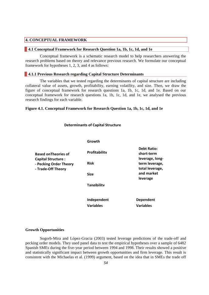
54
4. CONCEPTUAL FRAMEWORK
4.1 Conceptual Framework for Research Question 1a, 1b, 1c, 1d, and 1e
Conceptual framework is a schematic research model to help researchers answering the
research problems based on theory and relevance previous research. We formulate our conceptual
framework for hypotheses 1, 2, 3, and 4 as follows:
4.1.1 Previous Research regarding Capital Structure Determinants
The variables that we tested regarding the determinants of capital structure are including
collateral value of assets, growth, profitability, earning volatility, and size. Then, we draw the
figure of conceptual framework for research questions 1a, 1b, 1c, 1d, and 1e. Based on our
conceptual framework for research questions 1a, 1b, 1c, 1d, and 1e, we analysed the previous
research findings for each variable.
Figure 4.1. Conceptual Framework for Research Question 1a, 1b, 1c, 1d, and 1e
Growth Opportunities
Sogorb-Mira and López-Gracia (2003) tested leverage predictions of the trade-off and
pecking order models. They used panel data to test the empirical hypotheses over a sample of 6482
Spanish SMEs during the five-year period between 1994 and 1998. Their results showed a positive
and statistically significant impact between growth opportunities and firm leverage. This result is
consistent with the Michaelas et al. (1999) argument, based on the idea that in SMEs the trade off
Tangibility
Debt Ratio: short-term leverage, long-term leverage, total leverage, and market leverage
Determinants of Capital Structure
Dependent
Variables
Independent
Variables
Size
Risk
Profitability
Growth
Based onTheories of Capital Structure : - Pecking Order Theory - Trade-Off Theory
55
between independence and financing availability is more pronounced and the major part of debt
financing is short term. Sogorb-Mira and López-Gracia (2003) argued that this positive sign could
be affected by the proxy used to measure growth opportunities (the proportion represented by
intangible assets over total assets), which included, according to Spanish accounting rules, a large
proportion of tangible assets, such as assets financed by leasing, patents, trademarks, etc., and
therefore constituted an imperfect measure of the cited variable.
According to the study of Huang and Song (2002), which contains the market and
accounting data from more than 1000 Chinese listed companies up to the year 2000, to document
the characteristics of these firms in terms of capital structure, concluded that the static trade-off
model seemed better than pecking order hypothesis in explaining the features of capital structure
for Chinese listed companies. They used sales growth rates to measure the past growth experience
and Tobin‟s Q to measure a firm‟s growth opportunity in the future. Their finding showed that
firms with a high growth rate in the past tended to have a higher leverage, while firms that had a
good growth opportunity in the future (a higher Tobin‟s Q) tended to have a lower leverage. They
further explained that firms with brighter growth opportunity in the future preferred to keep
leverage low so they would not give up profitable investment because of the wealth transfer from
shareholders to creditors, also the fast growth firms meant that these firms had good investment
opportunities in the past and had used more debt to finance their investment 1.
Pandey (2001) examined the determinants of capital structure of Malaysian companies
using data from 1984 to 1999. He classified data into four sub-periods that corresponded to
different stages of the Malaysian capital market. Debt was decomposed into three categories:
short-term, long-term, and total debt. Both book value and market value debt ratios were
calculated. The results of pooled OLS regressions showed that growth variable had positive
significant influence on all types of book and market value debt ratios. This finding supports both
trade-off and pecking order theories. He further explained that Malaysian firms have higher short-
term than long-term debt ratios. Thus, it seems that they employ short-term debt to finance their
growth.
Sbeiti (2010) found a negative relation between growth opportunities and leverage and it
was consistent with the predictions of the agency theory that high growth firms used less debt,
since they did not wish to be exposed to possible restrictions by lenders. His explanation was that
growing firms had more options of choosing between risky and safe sources of funds and
managers as agents to shareholders went for risky projects in order to maximise the return to their
shareholders. Creditors, however, would be reluctant to provide funds to such firms as they would
bear more risk for the same return. They would thus demand a higher premium from growing
firms. Faced with this prospect and in order to avoid the extra cost of debt, growing firms will tend
to use less debt and more equity. Hence, the relatively large magnitude of the growth coefficient
may be indicative of a higher degree of information asymmetries in these markets, restricting the
ability of managers to raise external debt capital. He further explains that it is also important to
note that the firm-specific coefficients (such as size, liquidity, profitability and tangibility) are
almost identical. However, variables such as market to book ratio reflect the capital market
valuation of the firm, which in turn is affected by the conditions of the capital market.
1 The Determinants of Capital Structure: Evidence from China Samuel G. H. Huang and Frank M. Song
56
Shah and Khan (2007) found that growth variable was significant at a 10% level and was
negatively related to leverage. As they expected, this negative coefficient of -0.0511 showed that
growing firms did not use debt financing. They concluded that their results were in conformity
with the result of Titman and Wessels (1988); Barclay, et al. (1995) and Rajan and Zingales
(1995). They explained that growing firms had more options of choosing between safe and risky
firms. Managers, being agent to shareholders, would try to go for risky projects and increased
return to shareholders. Creditors would be unwilling to give funds to such firms as they would
bear more risk for the same return. To compensate for the additional risk in growth companies,
creditors would demand a risk premium. Facing extra cost of debt, growing firms would use less
debt and more equity.
Shah and Khan (2007) further explained that, since growing firms ran more risk of
project failure as compared to businesses that were static and were run in conventional ways,
managers might not want to add financial risk in addition to the high operational risk of the new
projects. Thus, the managers' unwillingness to add financial risk to firm resulted in lower debt
ratio for growing firms. Çağlayan and Şak (2010), on the other hand, found that market to book
has positive effect on book leverage found that market to book has positive effect on book
leverage.
A positive sign of the market to book was also along the lines of the pecking order theory.
They explained that theoretical expectations about the relationship of size and leverage, on the
other hand, was ambiguous. Han-Suck Song (2005) either expected a positive relationship between
expected growth and leverage, due to higher demand for funds, or a negative relationship, due to
higher costs of financial distress. However, the results they obtained here showed that there existed
no relationship between expected growth and leverage that was of economic significance. They
indicated that one possible explanation might be the effects of the two different theories
neutralising each other, the measurement used here, the percentage changed in total assets did not
reflect future growth possibilities, only past growth. Thus, other more significant results might be
obtained by using another measure for expected growth, for instance market-to-book ratio, a
commonly used proxy for expected growth.
The study of Gaud, Jani, Hoesli and Bender (2003), found the negative sign of growth
and confirmed the hypothesis that firms with growth opportunities were less levered. To analyse
this relationship further, they divided their sample in two sub-samples using the median growth as
cut-off. The negative sign and significance of the coefficient remained irrespective of the leverage
measure for the high growth firms. Concerning the low growth firms, which were typically no
growth firms as the market-to-book ratio was below one, they observed a negative relationship
between growth and leverage when market values were used, and a positive relation when
leverage was measured with book values.
Drobetz and Fix (2003) tested leverage predictions of the trade-off and pecking order
models using Swiss data. They found that firms with more investment opportunities applied less
leverage, which supported both the trade-off model and a complex version of the pecking order
model. They found that among all proxy variables, the strongest and most reliable relationship was
between investment opportunities and leverage. They explained that companies with high market-
to-book ratios had significantly lower leverage than companies with low market-to-book ratios.
Their result was consistent with both the trade-off theory and the extended version of the pecking
order theory.
Sogorb-Mira and López-Gracia (2003) tested leverage predictions of the trade-off and
pecking order models using Spanish data. They found that firms with more investment

57
opportunities applied less leverage, which supported both the trade-off model and a complex
version of the pecking order model.
According to Pandey (2001), the multivariate-pooled OLS regression results showed that
the coefficient of investment opportunity (market-to-book value ratio) variable was insignificant
throughout. This contradicted the pecking order theory of Myers (1977, 1984) that suggested that
companies with high market-to-book value would have lower long-term debt ratios because of the
problem of under-investment. However, his correlation matrix showed that investment opportunity
variable had inverse relation with book and market value short-term debt and long-term debt
ratios. He explained that correlation implied firms with larger investment opportunities were
perceived by lenders to have higher risk (bankruptcy costs).
Therefore, our hypothesis 1 is as follows.
Hypotheses 1a: “As implied by the trade-off theory and the pecking order theory, we
hypothesise that growth opportunity is positively related to debt ratios”.
Profitability
Drobetz and Fix (2003) tested leverage predictions of the trade-off and pecking order
models using Swiss data. Their results confirmed the pecking order model but contradicted with
the trade-off model, more profitable firms used less leverage. They found that profitability was
negatively correlated with leverage, both for book and market leverage. This result reliably
supported the predictions of the pecking order theory. According to Huang and Song (2002), the
results were consistent with the predictions of theoretical studies and the results of previous
empirical studies. Profitability had strong negative relation with total liabilities ratios.
Pandey (2001) results showed that profitability had a significant inverse relation with all
types of book and market value debt ratios. He showed that the results confirmed findings of
earlier studies and were consistent with pecking order theory (Myers, 1984) that postulated a
negative relationship between profitability and debt ratio. The negative relationship between
profitability and debt ratios contradicted with the tax shield hypothesis. He also showed that
profitability seemed to be the most dominant determinant of debt ratios of Malaysian firms as it
generally had high beta coefficients and t-statistics that were significant at 1% level of
significance.
Rebel A. Cole (2008) measured profitability by the winsorised return on assets, and
showed a consistent negative relation with the loan-to-asset ratio. The coefficients for ROA were
significant at the 0.05 level for three of the four surveys, with 1998 being the exception. As a
robustness test, they replaced return on asset with a simple zero-one indicator for profitable firms.
They found that this variable had a negative and highly significant coefficient in each of the four
surveys. These latter findings were strongly supportive of the pecking order theory, which
predicted that profitable firms used less debt because they could fund projects with retained
earnings, but it was inconsistent with the trade-off theory, which predicted that profitable firms
used more debt to take advantage of the debt tax shield, and because they had lower probability of
financial distress.
Sbeiti (2010) found that firm profitability seemed to have a statistically negative and
significant relationship with both the book and market leverage in the three countries. The
negative coefficient of profitability was indicative of the presence of informational asymmetries
which could lead to higher external financing premiums and pecking order behaviour under which
58
firms preferred internal financing from external, but it may also support the view that the lack of
well-developed financial markets forces firms to rely mostly on internal financing.
He further explained that the latter explanation was consistent with Booth et al. (2001)
who reported the same results for the profitability variable and argued that the importance of
profitability was related to the significant agency and informational asymmetry problems in
developing countries. Booth et al. (2001) indicated that it was also possible that profitability was
correlated with growth opportunities so that the negative correlation between profitability and
leverage, proxied the difficulty in borrowing against intangible growth opportunities. Thus, firms
that generated relatively high internal funds generally tended to avoid gearing. The results were
also consistent with Titman and Wessels (1988), Rajan and Zingales (1995), Cornelli et al. (1996),
Bevan and Danbolt (2002) in developed countries, Pandey (2001), Um (2001), Wiwattanakantang
(1999), Chen (2004), Deesomsak, Paudyal and Pescetto (2004) and Antoniou et al. (2007).
In the Shah and Khan (2007) study, the most important explanatory variable was beyond
doubt the profitability variable which had a very high t-statistics of -21.68 and p-value of 0.0000.
The coefficient was -0.7945. The negative sign and statistical significance validated the acceptance
of our fourth hypothesis. The prediction of information asymmetry hypothesis by Myers and
Majluf (1984) was approved by the negative sign whereas the predictions of bankruptcy theory
and free-cash flow hypothesis by Jensen (1984) were not substantiated. It was thus proved that the
pecking order theory dominated trade-off theory. Frydenberg (2001b) describes retained earning as
the most important source of financing. Good profitability thus reduces the need for external debt.
Shah and Khan (2007) explanations were as follows: One possible bias in the finding
could come from the fact that many firms were family controlled in Pakistan. They inflated the
cost of production and the controlling shareholders took out profit in forms other than dividend.
The result was the unreal negative profit figure in income statement. The year to year negative
profit figure reduced the owner‟s equity and increased the debt percentage in overall financing. In
their initial sample, 32% of all observations for profit were negative. Even though they removed
outliers from our analysis that were 3 standard deviations from the overall mean, still they had a
20.1% negative observation for the profitability variable. This was also evident from the fact that
the average profitability ratio was negative for four industries in the sample years. To check for
this bias, they removed all observation of negative profitability and ran regression, the coefficient
for profitability was still negative, but this time the p-value was 0.83 against a very small t-value
of -0.17. This showed that profitability has no significant relationship with leverage. This is why
the results of their main regression model should be interpreted with care with regard to
profitability.
In the Çağlayan and Şak (2010) study, the paper examined the capital structure of banks,
from the perspective of the empirical capital structure literature, for non-financial firms by using
the panel data analysis method ; investigated which capital structure theories could explain the
capital structure choice of the banks; and identified two sub-periods to determine the differences
across determinants of capital structure in the different periods for Turkish banks after the
financial crises and restructuring periods. Their findings showed that profitability was found to
have negative effect on the book leverage. A negative relationship between profitability and
leverage was observed in the majority of empirical studies. This study provided similar results
confirming the pecking order theory rather than static trade-off theory.
In the Han-Suck Song (2005) study, they found that profitability was negatively
correlated with all three leverage measures, which was in line with the pecking-order theory; firms
preferred using surplus generated by profits to finance investments. Han-Suck Song (2005)
explained that the result might also indicate that firms in general preferred internal funds rather
59
than external funds, irrespective of the characteristic of an asset that should be financed (e.g.
tangible or non-tangible asset).
Gaud, Jani, Hoesli, and Bender (2003) concluded that as reported in several other studies,
the profitability variable was negative and significant in all cases (Rajan and Zingales, 1995;
Booth et al. , 2001; Frank and Goyal, 2002). This finding provides support for the pecking order
theory.
As the contradiction of the pecking order theory and the trade-off theory and also previous
research findings, we hypothesise that:
Hypothesis 1b: “As the pecking order hypothesis, we hypothesise that profitability has a
negative relationship with debt ratios and, based on the trade-off theory, we hypothesise that
profitability has a positive relationship with debt ratio”.
Risk
Drobetz and Fix (2003) found, as expected, the relationship between leverage and
volatility negative. They also showed that their finding supports both the trade-off theory (more
volatile cash flows increased the probability of default) and the pecking order theory (issuing
equity was more costly for firms with volatile cash flows). Huang and Song (2002) results showed
that there was the positive relation between total liabilities ratio and volatility. It was consistent
with Hsia‟s (1981) view that firms with higher leverage level tended to make riskier investment.
They found that the companies with high leverage in China tended to make riskier investments.
They further explained that in China, the credit market was still regulated and the term structures
of interest rates were decided by the central bank rather than by the market force such as the
borrower‟s credibility. Banks only had the right to decide whether borrower‟s application was
approved or not and the listed companies generally were regarded as best companies in China. As
a result, the companies with high business risk still could get bank loans at regulated interest rate,
which was lower than market rate if interest rate was deregulated.
Pandey (2001) found that there was a negative relation of earnings volatility with book
and market value long-term debt ratio, which was consistent with the trade-off theory. And it also
revealed a positive relation between risk and short-term debt ratios. In Shah and Khan (2007)
study, the coefficient for earning volatility was 0.0000 and had a very large p-value of 0.869. They
explained that volatility of income had no impact on the debt level. The magnitude of earning
volatility was a sign of expected bankruptcy. Firms with higher volatility were considered risky
because they could go bankrupt. The cost of debt for such firm should be more and thus, these
firms would employ low level of leverage. They further added that court processes were slow in
Pakistan and there were very few cases of bankruptcy, this could be the possible explanation for
the insignificant relationship between earning volatility and leverage. Creditors did not consider
the income source or the variation in income for the repayment of loan and interest by the firm.
They relied more on the security of fixed assets.
Han-Suck Song (2005) revealed that the effect of income variability on debt was
approximately zero, but still statistically significant. Lööf (2003) also obtained similar results,
according to him, this might be due to the fact that the time period studied (1991 to 1998; this
study: 1992 to 2000) coincided with a period of strong economic recovery and a generally positive
trend in revenues. Gaud, Jani, Hoesli and Bender (2003) concluded that the positive impact of risk
for the fixed effects estimation when using market data implied that firms, which performed below
60
average, were less levered. In other words, companies with a high operating risk tried to control
total risk by limiting financial risk.
Based on the same prediction of the theories but with slightly different reason, our
hypothesis is as follows.
Hypotheses 1c: “In accordance with the pecking order theory and trade-off theory, we
hypothesise a negative relationship between risk (earnings volatility) and debt ratio”.
Size
Drobetz and Fix (2003) found that size was positively related to leverage, indicating that
size was a proxy for a low probability of default. However, the estimated coefficients on size were
generally not significant. They also found that it was in contrast to the results in Rajan and
Zingales (1995), where firms in Germany tended to be liquidated more easily than in the Anglo-
Saxon countries. Large firms had substantially less debt than of small firms. Therefore, Drobetz
and Fix (2003), interpreted their results for Switzerland as size being a proxy for low expected
costs of financial distress, where small firms in Switzerland were especially wary of debt. Again,
they concluded that this result supported the trade-off theory, suggesting that large firms exhibited
lower probability of default.
Sogorb-Mira and López-Gracia (2003) found that firm size and leverage were found to be
positively related. They explained that this relationship could come from the fact that small-
medium enterprise (SMEs) had to face higher bankruptcy costs, greater agency costs and bigger
costs to resolve the higher informational asymmetries. Even within this firm category, SMEs of
greater size could access a higher leverage. They also found that this result was the same as that
obtained by a considerable number of previous studies (Ocaña et al. , 1994; Hutchinson, 1995;
Chittenden et al. , 1996; Berger and Udell, 1998; Michaelas et al. , 1999; Romano et al. , 2000).
Huang and Song (2002) concluded that, on the relationship between size and leverage, if
size was interpreted as a reversed proxy for bankruptcy cost, it should have less or no effect on
Chinese firms‟ leverage because the state kept around 40% of the stocks of these firms and,
because of soft budget constraint, state-controlled firms should have much less chance to go
bankrupt. They argued that although the state was still a controlling shareholder for most listed
firms, these firms were limited corporations; it was unlikely that the state would bail them out,
even in case of trouble, because the central government was only a legal representative of state
shareholder. The beneficiaries of state shares in these listed firms might be local governments,
who could behave just like big private shareholders. They believed the economic force worked
quite well even in an environment where the state was the controlling shareholder.
Pandey (2001) found that size was positively related to all types of book and market
value debt ratios and all of coefficients were significant at 0.01level of significance. He showed
that the positive correlation between size and debt ratios confirmed the hypothesis, that larger
firms tended to be more diversified and less prone to bankruptcy and the direct cost of issuing debt
or equity was smaller. This is consistent with the trade-off theory.
Rebel A. Cole (2008) investigated firm size, as measured by the natural logarithm of total
assets, and found size was inversely related to firm leverage, and this relation was significant at
better than the 0.001 level in each survey. He explained that larger firms used significantly less
debt in their capital structure, and his result was at odds with what Frank and Goyal (2006) cited as
one of the “core set of seven factors that are correlated with cross-sectional differences in
leverage.” Cross-sectional studies of publicly traded firms found that leverage was “robustly
61
related” to firm size, as measured by the log of assets. He added that, clearly, this result did not
hold for privately held firms. This result also is inconsistent with the trade-off theory, which
predicts larger firms should use more leverage than smaller firms.
Sbeiti (2010) investigated the determinants of capital structure in the context of three
GCC countries and the impact of their stock markets' developments on the financing choices of
firms operating in these markets. He found that the coefficient values of the size variable remained
positive and were statistically significant in relation to both book and market leverage ratios across
the three countries. These results confirmed the importance of the size variable as a determinant of
the capital structure decisions of firm operating in the GCC markets.
He added that his result was in line with the results reported by Rajan and Zingales
(1995), Wiwattanakantang (1999), Booth et al. (2001), Pandey (2001), Prasad et al. (2001),
Deesomsak, Paudyal and Pescetto (2004), Antoniou et al. (2007), the size of the coefficient was
positive and statistically significant in the case of all three countries and for both measures of
leverage. He explained that these results were consistent with the theoretical prediction that larger
firms tended to be more diversified, less prone to bankruptcy with smaller direct cost for issuing
debt or equity. If size was a proxy for the inverse probability of bankruptcy, then the positive
relation between size and leverage complied with the predictions of the trade-off theory. This is
because larger firms can diversify their investment projects on a broader basis and limit their risk
to cyclical fluctuations in any one particular line of production. Moreover, informational
asymmetries tend to be less severe for larger firms than for smaller ones; hence, larger firms find it
easier to raise debt finance. It is also noticed that size seems to have only a limited impact on the
capital structure of firms in Oman as compared to Kuwaiti and Saudi Arabia firms. This result may
indicate smaller differences in informational asymmetries between large and small companies in
Oman.
In Shah and Khan (2007) study, size had a positive coefficient but was insignificant, with
the coefficient value of 0.0002, the very small t-value of 0.07, and the p-value of 0.940. They
showed that size variable was not a proper explanatory variable of debt ratio. Their second
hypothesis was based on the Rajan and Zingales‟ (1995) argument that there was less asymmetric
information about the larger firms which reduced the chance of undervaluation of new equity.
Their finding did not confirm to the Titman and Wessels‟ (1988) argument as well that larger firms
were more diversified and have lesser chances of bankruptcy that should motivate the use of debt
financing.
Shah and Khan (2007) explained why their finding on size of a firm with relation to the
leverage ratio did not confirm to the established theories. Trade off theory suggested that firm size
should matter in deciding an optimal capital structure because bankruptcy costs constituted a small
percentage of the total firm value for larger firms and greater percentage of the total firm value for
smaller firms. As debt increased the chances of bankruptcy, hence smaller firms should have lower
debt ratio. In case of Pakistan, the court process was very slow. Negative equity figure in the
balance sheet of a firm year after year and the firm still managed to survive. Among total
observations of equity figure, 15% were in negative. This meant that firms were not much fearful
of bankruptcy. They managed to survive even with negative equity figure. In the given scenario,
size was not a matter. Facing no or very low bankruptcy costs, firms would employ debt regardless
of its size.
They further explained that initial public offerings are negligible in Pakistan both for
small and large firms. There were only a few cases of selling ownership in government owned
enterprises to public in the recent past. It meant that size was not the determinant of new equity
62
issue rather other factors like family control, capital market development, managerial control, etc.,
determine the issue of new equity. Hence, Shah and Khan (2007) concluded that size should not
necessarily be a significant determinant of leverage ratio.
Rajan and Zingales(1995) argued that the problem of undervaluation of new equity issue
for large firm was not severe as there was less information asymmetry about them. Hence size
should be negatively related to leverage. Çağlayan and Şak (2010) research concluded that size
was found to have positive relationships with the leverage of banks. The findings of the
relationship with the size were in line with the static trade-off and agency cost theory.
In the Han-Suck Song (2005) study, the result revealed that size was a significant
determinant of leverage. They explained that while size was positively related to both total debt
and short-term debt ratio, it was negatively correlated with long-term debt ratio, although, the
economic significance was rather small for the latter case. They added that even if the data did not
allow them to further decompose short-term debt, they might still find the results of Bevon and
Danbolt (2000) interesting. They found that while size was positively correlated with both trade
credit and equivalent and short-term securitized debt, it was negatively correlated with short-term
bank borrowing. This might indicate that small firms were supply constrained, in that they did not
have sufficient credit ranking to allow them to long-term borrowing.
Gaud, Jani, Hoesli, and Bender (2003) analysed the determinants of the capital structure
for a panel of 106 Swiss companies listed in the Swiss stock exchange. Both static and dynamic
tests were performed for the period 1991-2000. They found that the size of companies, the
importance of tangible assets and business risk were positively related to leverage, while growth
and profitability were negatively associated with leverage. The sign of these relations suggested
that both the pecking order theory and trade off hypothesis were at work in explaining the capital
structure of Swiss companies, although more evidence existed to validate the latter theory. Their
analysis also showed that Swiss firms adjusted toward a target debt ratio, but the adjustment
process was much slower than in most other countries.
Gaud, Jani, Hoesli, and Bender (2003) found positive impact of size on leverage. They
explained that it was consistent with the results of many empirical studies (Rajan and Zingales,
1995; Booth et al., 2001; Frank and Goyal, 2002). It led them to reject the hypothesis that size
acted an inverse proxy for informational asymmetries, but could suggest that size acted an inverse
proxy for the probability of bankruptcy. They added that the variable size was not significant any
more when leverage was computed with long-term debt only. One possible explanation from them
was that large companies had easier access to the bond markets (Ferri and Jones, 1979). The
development of financial markets has pushed large companies to search for better credit
conditions. Consequently, there has been a tendency for banks to grant more loans to small and
medium size companies. The market for short term debt securities is not well developed in
Switzerland. This allows banks to select between borrowers. As banks will prefer large firms to
small ones, the sign of the size coefficient is positive.
For these differences, we test the following hypothesis.
Hypotheses 1.d: “As suggested by the trade-off theory, we hypothesise that size has a positive
relationship with debt ratio, and as suggested by the pecking order theory of the capital
structure there is a negative relationship between debt ratio and size”.
Tangibility
63
Drobetz and Fix (2003), found that tangibility was almost always positively correlated
with leverage. They showed that the regression coefficient on tangibility was significant in about
half of all regressions and this supported the prediction of the trade-off theory that the debt-
capacity increased with the proportion of tangible assets on the balance sheet. Sogorb-Mira and
López-Gracia (2003) tested leverage predictions of the trade-off and pecking order models using
Spanish data. They showed that at an aggregate level, leverage of Spanish firms was
comparatively low, but the results depended crucially on the exact definition of leverage. The
result confirmed the pecking order model but contradicted with the trade-off model.
Huang and Song (2002) found that, in contrast to theoretical predictions, tangibility was
negatively related with total liability. They explained that the reason for that might be the non-debt
part of total liability did not need collaterals. Long-term debt ratio was positively correlated with
tangibility. Pandey‟s results (2001) indicated a significant negative relation of tangibility (fixed
asset to-total asset ratio) with book and market value short-term debt ratios. The relation of
tangibility with the market value long-term debt ratio was also significantly negative while with
the book value long-term ratio, it was not statistically significant. These results contradicted the
trade-off theory that postulated a positive correlation between long-tem debt ratio and tangibility
since fixed assets act as collateral in debt issues. He also concluded that his results were consistent
with DeAngelo and Masulis (1980) who suggested an inverse correlation between tangibility and
debt ratio.
Rebel A. Cole (2008) studied the tangibility, as measured by the ratio of property, plant
and equipment to total assets. The result was positive across each of the four surveys and was
statistically significant at better level than the 0.05 level for each survey except for the result in
2003. The coefficients ranged from 0.073 to 0.171, indicating that a 100 basis point increased in
the tangible asset ratio was associated with a 7.3 to17.1 basis point increase in the loan-to-asset
ratio. According to Frank and Goyal (2006), the relation between tangibility and leverage was
reliably positive in cross-sectional studies of publicly traded firms. Their results for privately held
firms were broadly consistent with this finding.
Sbeiti (2010) found that the stylized fact that the tangibility variable was positively
related to the availability of collateral and leverage was not consistent with the findings in the
paper, where tangibility was negative and statistically significant in relation to both book and
market value of leverage in the three countries. She added that this negative association between
leverage and tangibility could be explained by the fact that those firms that maintained a large
proportion of fixed assets in their total assets tended to use less debt than those which did not. This
could be due to the fact that a firm with an increasing level of tangible assets might have already
found a stable source of income, which provided it with more internally generated funds and
avoided using external financing.
She further explained that another explanation for this relationship could be the view that
firms with higher operating leverage (high fixed assets) would employ lower financial leverage,
and overall the results were consistent with Cornelli et al. (1996), Hussain and Nivorozhkin
(1997), Booth et al. (2001), and Nivorozhkin (2002) who also suggested a negative relation
between tangibility and debt ratio. Finally, the relatively larger coefficient value of tangibility for
the Saudi firms might indicate that firms in this country had an effective guarantee against
bankruptcy.
In Shah and Khan (2007) study, they used two variants of panel data analysis, attempted
to find the determinants of capital structure of listed none-financial firms for the period 1994-
2002. Pooled regression analysis was applied with the assumption that there were no industry or

64
time effects. They used six explanatory variables to measure their effect on leverage ratio. Three
of their variables were significantly related to leverage ratio whereas the remaining three variables
were not statistically significant in having relationship with the debt ratio. Their results approved
the prediction of trade-off theory in case of tangibility variable whereas the earning volatility and
depreciation variables failed to confirm to trade-off theory. The growth variable confirmed the
agency theory hypothesis whereas profitability approved the predictions of pecking order theory.
Size variable neither confirmed to the prediction of trade-off theory nor to asymmetry of
information theory.
Shah and Khan (2007) found that tangibility, with a coefficient of 0.1304 was
significantly related to debt. It had the second highest t-value of 5.56 against a very low p-value of
0.0000. This showed that tangibility was one of the most important determinants of leverage ratio
in Pakistan. Thus their first hypothesis was confirmed by the statistically significant positive
relationship between tangibility and leverage. This finding was in contrast to the earlier finding by
Shah and Hijazi (2004). They found that tangibility was not significantly related to leverage ratio.
Çağlayan and Şak (2010) investigated the relationship between tangibility and book
leverage, and it was found to be negative in this study. They explained that this significant
negative relationship between tangibility and leverage provided further support for the agency cost
theory and the existence of conflict between debt holders and shareholders.
In Han-Suck Song (2005) study, the paper analysed the explanatory power of some of the
theories that have been proposed in the literature to explain variations in capital structures across
firms. In particular, this study investigated capital structure determinants of Swedish firms based
on a panel data set from 1992 to 2000 comprising about 6000 companies. Swedish firms were on
average very highly leveraged, and furthermore, short-term debt comprised a considerable part of
Swedish firms‟ total debt. An analysis of determinants of leverage based on total debt ratios might
mask significant differences in the determinants of long and short-term forms of debt. Therefore,
their paper studied determinants of total debt ratios as well as determinants of short-term and long-
term debt ratios. The results indicated that most of the determinants of capital structure suggested
by capital structure theories appeared to be relevant for Swedish firms.
The coefficients of tangibility are highly statistically significant for all three debt
measures. But while the results show that tangibility has a positive relationship with total debt
ratio and long-term debt ratio, as expected according to the theoretical discussion above,
tangibility is negatively related to the short-term debt ratio. This finding is consistent with the
results of Bevan and Danbolt (2000), Huchinson et al. (1999), Chittenden et al. (1996) and the
Van der Wijst and Thurik (1993) report (see also Michaleas et.al., 1999).
Gaud, Jani, Hoesli, and Bender (2003) concluded that the coefficient of the TANG
variable was positive and significant for the panel data estimations, and this result was similar to
those reported in previous research (Rajan and Zingales, 1995; Kremp et al., 1999; Frank and
Goyal, 2002). Their result suggested that firms used tangible assets as collateral when negotiating
borrowing, especially long term borrowing. The observed sign of the relationship did not confirm
the sign that would be expected when using the pecking order theory framework. In such a
framework, firms with smaller tangible assets were more subject to informational asymmetries,
and were more likely to use debt - principally short term debt - when they needed external
financing.
Our hypothesis, based on theory and previous research, is as follow.
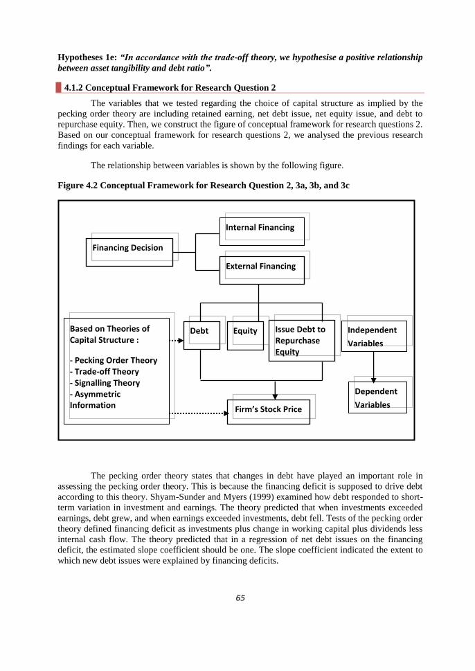
65
Hypotheses 1e: “In accordance with the trade-off theory, we hypothesise a positive relationship
between asset tangibility and debt ratio”.
4.1.2 Conceptual Framework for Research Question 2
The variables that we tested regarding the choice of capital structure as implied by the
pecking order theory are including retained earning, net debt issue, net equity issue, and debt to
repurchase equity. Then, we construct the figure of conceptual framework for research questions 2.
Based on our conceptual framework for research questions 2, we analysed the previous research
findings for each variable.
The relationship between variables is shown by the following figure.
Figure 4.2 Conceptual Framework for Research Question 2, 3a, 3b, and 3c
The pecking order theory states that changes in debt have played an important role in
assessing the pecking order theory. This is because the financing deficit is supposed to drive debt
according to this theory. Shyam-Sunder and Myers (1999) examined how debt responded to short-
term variation in investment and earnings. The theory predicted that when investments exceeded
earnings, debt grew, and when earnings exceeded investments, debt fell. Tests of the pecking order
theory defined financing deficit as investments plus change in working capital plus dividends less
internal cash flow. The theory predicted that in a regression of net debt issues on the financing
deficit, the estimated slope coefficient should be one. The slope coefficient indicated the extent to
which new debt issues were explained by financing deficits.
External Financing
Internal Financing
Financing Decision
Issue Debt to Repurchase Equity
Equity Debt
Firm’s Stock Price
Based on Theories of Capital Structure :
- Pecking Order Theory - Trade-off Theory - Signalling Theory - Asymmetric Information
Dependent
Variables
Independent
Variables
66
Shyam-Sunder and Myers found strong support for pot prediction in a sample of 157
large firms. The coefficient was 0.75 with an R2 of 0.68. They interpreted this evidence to imply
that “pecking order was an excellent first order descriptor of corporate financing behavior”
(Shyam-Sunder and Myers, 1999).
Previous research from Indonesia, Ari Christianti (2008), concluded that: (1) The results
of this study did not fully support the pecking order theory in explaining the behaviour of firms
financing in the Indonesia Stock Exchange (IDX) especially the manufacturing sector. This could
be explained from the results of the estimation that showed a negative and significant coefficient
of pecking order. (2) It may be explained from the results of this study, is the Indonesian capital
market conditions that are different from capital markets in developed countries studied by
Shyam-Sunder and Myers (1999), Frank and Goyal (2003) and Jong, Verbeek, and Verwijmeren
(2005). In addition, the impact of economic crisis in 1997 still affected the economic condition of
Indonesia until 2005.
Previous research from other country: Leary and Roberts (2005) empirically examined
the pecking order theory of capital structure using a new empirical model that was motivated by
the pecking order's decision rule and implied financing hierarchy. A power study of their
associated hypothesis test revealed that the test could distinguish pecking order behaviour from
non-pecking order behaviour, as well as quantify the degree to which firms adhered to the
financing hierarchy. They found that 62% (29%) of the firms in the sample were following the
pecking order in their decision between internal and external (debt and equity) financing and that
most of the equity issuing violations were not due to debt capacity concerns, as suggested by the
modified version of the pecking order. Leary and Roberts (2005) showed empirically that the
pecking order did not seem to be an implication of information asymmetry.
Francisco Sogorb-Mira and José López-Gracia (2003) explored two of the most relevant
theories that explained financial policy in small and medium enterprises (SMEs): pecking order
theory and trade-off theory. Panel data methodology was used to test the empirical hypotheses
over a sample of 6482 Spanish SMEs during the five-year period 1994–1998. Their results
suggested that both theoretical approaches contributed to explain capital structure in SMEs.
However, while they found evidence that SMEs attempted to achieve a target or optimum leverage
(trade-off model), there was less support for the view that SMEs adjusted their leverage level to
their financing requirements (pecking order model). Cotei and Farhat (2008) investigated the
models used in testing the trade-off and pecking order theories. Specifically, for the pecking order
theory, they examined the symmetric behaviour assumption. For the pecking order model, the test
results rejected the symmetric behaviour assumption at the industry level as well as across all
industries.
Under the pecking order model, firms in financing deficit used debt to finance their new
investment, whereas firms in financing surplus ended up retiring debt rather than repurchasing
equity. Hence, their results showed that for the pecking order model, they rejected the hypothesis
that firms had a symmetric behaviour regardless of the sign of the financing variable. Their results
showed that firms had the tendency to reduce debt by a significantly higher proportion when they
had financing surplus compared to the proportion of debt issued when they had financing deficit.
Joher, Ahmed, and Hisham (2009) paper drew on studies from finance and accounting
literature to revisit pecking order and static trade-off-hypothesis in the context of the Malaysia
capital market, using a sample of 102 list firms over a four-year time frame (1999-2003). Their
evidence from the pecking order model suggested that the internal fund deficiency was the most
important determinant that possibly explained the issuance of new debt. Hence, the pecking order

67
hypothesis was well explained in the Malaysian capital market despite the lower predicting power.
This could be the evidence from both pecking order models that exhibited a significant coefficient
for financing deficit, significant at the conventional level, but with very low R2. To address this
issue of low predicting power, the pecking order model was expanded by including the component
of internally generated fund deficiency such as dividend, debt repayment, capital expenditure,
investment on working capital and operating cash flow. The expanded pecking order model
provided more vibrant explanation for debt issuance with higher predictive power.
Meanwhile, their result for static trade-off-model was not fit to explain the issuance of
new debt issue in Malaysian capital market. That was an interesting findings that confirmed the
fact that Malaysian firms did not too much care about tax-shield benefit derived from employing
both debt and non-debt tax-shields. The firm‟s size, which was used to neutralise the size effect,
appeared to provide some explanation for the variation in its capital structure policy choice.
In the Bharath, Pasquariello, and Wu (2008) study, using a novel information asymmetry
index based on measures of adverse selection developed by the market microstructure literature,
they tested whether information asymmetry was an important determinant of capital structure
decisions, as suggested by the pecking order theory. They found that information asymmetry did
affect the capital structure decisions of U.S. firms over the sample period 1973–2002. Overall, this
evidence explained why the pecking order theory was only partially successful in explaining all of
firms‟ capital structure decisions.
The Shyam-Sunder and Myers (1994) paper tested traditional capital structure models
against the alternative of a pecking order model of corporate financing. The basic pecking order
model, which predicted external debt financing driven by the internal financial deficit, had much
greater explanatory power than a static trade-off model which predicted that each firm adjusts
toward an optimal debt ratio. They summarized main conclusions regarding pot as follows: (1)
The pecking order is an effective first-order descriptor of corporate financing behaviour. (2) The
coefficient and significance of the pecking order variable change hardly at all. (3) The strong
performance of the pecking order does not occur just because firms fund unanticipated cash needs
with debt in the short run. Their results indicated that firms planned to finance anticipated deficits
with debt.
Medeirosa and Daherb tested two models with the purpose of finding the best empirical
explanation for the capital structure of Brazilian firms. The models tested were developed to
represent the static tradeoff theory and the pecking order theory. The sample consisted of firms
listed in the São Paulo (Brazil) stock exchange from 1995 through 2002. By using panel data
econometric methods, they aimed at establishing which of the two theories had the best
explanatory power for Brazilian firms. The analysis of the outcomes led to the conclusion that the
pecking order theory provided the best explanation for the capital structure of those firms.
The pecking order theory established that the financial deficit was covered by debt,
permitting the issue of new shares in exceptional cases only. The Frank and Goyal model stated
that the deficit coefficient must be equal to zero in order to validate the strong form of the pecking
order theory. Therefore, the most important test was the one which determined the value of this
coefficient. The results obtained in Medeirosa and Daherb study supported the pecking order
theory in its semi-strong form, since both the aggregate and the disaggregate equations were led to
accept the null that the slopes were equal to one, but to reject the null that the intercepts were equal
to zero.
68
The Lakshmi Shyam-Sunder and Stewart C. Myers (1999) paper tested traditional capital
structure models against the alternative of a pecking order model of corporate financing. The basic
pecking order model, which predicts external debt financing driven by the internal financial
deficit, has much greater timeseries explanatory power than a static tradeoff model, which predicts
that each firm adjusts gradually toward an optimal debt ratio.
Instead, they view the theories as contending hypotheses and examine their relative
explanatory power. The attention to statistical power is an important methodological point. They
summarized the main conclusions regarding pot as follows. (1) The pecking order is an excellent
first-order descriptor of corporate financing behaviour, for their sample of mature corporations. (2)
The strong performance of the pecking order does not occur just because firms fund unanticipated
cash needs with debt in the short run. Their results suggested that firms planned to finance
anticipated deficits with debt.
Therefore, our hypothesis 2 is as follows:
Hypothesis 2: “Firms in the manufacturing sector raise capital for investments externally (with
debt, equity, or debt to repurchase equity)”.
4.1.3 Conceptual Framework for Research Question 3
The variables that we tested regarding the effect of capital structure choices on stock
price as implied by some theories are including firm‟s stock price, net debt issue, net equity issue,
or issue debt to repurchase equity. Then, we construct the figure of conceptual framework for
research questions 3. Based on our conceptual framework for research questions 3, we analysed
the previous research findings for each variable. The relationship between variables is shown by
the figure 4.2.
When a firm issues, repurchases or exchanges one security for another, it changes its
capital structure. There are several theories which explain the relationship between capital
structure and stock price.
Theories which explain the relationship between net debt and equity issue and stock price
are as follow.
Net Debt Issue
Theories implied different implication for the issuance of new debt on firm‟s stock price.
Ross (1977) introduces the notion of signalling in the capital structure theory. According to his
theory, the managers know the true distribution of the company returns, but investors do not. He
argues that higher financial leverage can be used by the managers to signal an optimistic future of
the company since the debt is a contractual obligation to repay both principal and interests. The
failure to make those payments could lead to bankruptcy and by consequence the managers would
lose their jobs. Therefore adding more debt to the capital structure could be interpreted as a good
signal of the managers‟ optimism about their companies.
The issuance that new debt will positively influence a firm‟s stock price is based on
signalling theory through capital structure, the increased level of leverage is accompanied by
higher risk of bankruptcy, the increased level of debt indicates the confidence of the management
in the future prospects of the firm. Hence, it carries greater conviction than a mere announcement
of undervaluation of the firm, by the management. The markets normally react favourably to
moderate increases in leverage.

69
On the other hand, the issuance of new debt will less negatively influence a firm‟s stock
price than the issuance of new equity, or no market reaction, is as implied by the pecking order
theory. The pecking order theory is usually interpreted as predicting that securities with less
adverse selection (debt) will result in less negative or no market reaction.
However, under the trade-off theory, the market response to a leverage change confounds
two pieces of information. Under the theory, firms will only take actions if they expect benefits.
The information contained in security issuance decisions could be either good news or bad news. It
would be good news if the firm is issuing securities to take advantage of a promising new
opportunity that was not previously anticipated. It might be bad news if the firm is issuing
securities because the firm actually needs more resources than anticipated to conduct operations. A
firm may also issue securities now in anticipation of a change in future needs. This implies that the
trade-off theory by itself places no obvious restrictions on the market valuation effects of issuing
decisions. Everything depends on the setting.
Net Equity Issue
Meanwhile, based on signalling theory, agency perspective, and pecking order theory, the
issuance of new equity will negatively influence a firm‟s stock price. As implied by signalling
through capital structure, an issue of equity is a signal that the firm is overvalued. The market
concludes that the management has decided to offer equity because it is valued higher than its
intrinsic worth by the market. The markets normally react negatively to fresh issue of equity.
Jung et al. (1996) suggested an agency perspective and argued that equity issues by firms
with poor growth prospects reflected agency problems between managers and shareholders. If this
is the case, then stock prices will react negatively to the news of equity issues. However, the
pecking order theory is usually interpreted as predicting that securities with more adverse selection
(equity) will result in more negative market reaction.
Myers and Majluf (1984) assumed that company managers have always more information
about the true value of the company than the other investors. Managers will therefore time a new
equity issue if the market price exceeds their own assessment of the stock value – if the stocks are
overvalued by the market. Since investors are aware of the existence of the information
asymmetry, they will interpret the announcement of an equity issue as a signal that the listed
stocks are overvalued, which subsequently will cause a negative price reaction. The managers can
use the information asymmetry to their profit and to reinforce their entrenchment strategy in their
respective companies. Besides, they can use their informational advantage in order to get more
benefits and to maximise their income (Stiglitz and Edlin, 1992). With this intention, the managers
can reduce the threat of the competition of the potential managers on the labor market by two
possible manners: either by setting up investments strongly dependent on their specific
information, or by investing in projects with high information asymmetry.
Based on the undervaluation hypothesis, stock repurchases offer flexibility not only for
distributing the excess of funds but also the timing of distributing these funds. This flexibility in
timing is beneficial because firms can wait to repurchase until the stock price is undervalued. The
undervaluation hypothesis is based on the premise that information asymmetry between insiders
and shareholders may cause a firm to be misvalued. If insiders believe that the stock is
undervalued, the firm may repurchase stock as a signal to the market or to invest in its own stock
and acquire mispriced shares. According to this hypothesis, the market interprets the action as an
indication that the stock is undervalued (Dittmar, 1999). Because of the asymmetric information
70
between managers and shareholders, share repurchase announcements are considered to reveal
private information that managers have about the value of the company (in Smura).
The information/signalling hypothesis has three immediate implications: repurchase
announcements should be accompanied by positive price changes; repurchase announcements
should be followed (though not necessarily immediately) by positive news about profitability or
cash flows; and repurchase announcements should be immediately followed by positive changes in
the market‟s expectation about future profitability (in Gustavo Grullon and Roni Michaely, 2002).
Some previous empirical evidence regarding to debt issue on stock price are the
following: Announcements of ordinary debt issues generate zero market reaction on average
(Eckbo (1986) and Antweiler and Frank (2006)). The zero market reaction to corporate debt issues
is robust to various attempts to control for partial anticipation.
Ross (1977) showed that good corporate performance could give a signal with a high
portion of debt in their capital structure. Ross (1977) assumed the firms that are less good
performance would not use debt in large portion as it would be followed by the high chance of
bankruptcy. By using these assumptions in which the company will use the good performance of
higher debt, while firms that are less good performance will use more of equity. Ross (1977)
assumed that investors would be able to distinguish the company's performance by looking at the
company's capital structure and they would give a higher value on the company with larger debt
portion. It indicated that the result did not support the stating of the signalling theory. The result
indicated that the greater the leverage, the greater the possibility of financial distress leading to
bankruptcy. When the company went bankrupt, shareholders would lose money they have invested
in the company (Peirson et al, 2002).
Exchange of common for debt/preferred stock generates positive stock price reactions
while exchange of debt/preferred for common stock generates negative reactions (Masulis, 1980a).
Summarising the event study evidence, Eckbo and Masulis (1995) concluded that announcements
of security issues typically generated a nonpositive stock price reaction.
In Indonesia, the regression coefficient between leverage and stock price is significantly
negative. The use of high leverage will be responded by the market with a fall in stock prices.The
results are consistent with the findings of a negative relationship between leverage and stock price
as proposed by Frank and Goyal (2003). Relationship between the two variables will be positive at
the time the company has many tangible assets that will secure leverage of companies.
Announcements of convertible debt issues result in mildly negative stock price reactions
(see Dann and Mikkelson (1984) and Mikkelson and Partch (1986)). The valuation effects are the
most negative for common stock issues, slightly less negative for convertible debt issues and least
negative (zero) for straight debt issues. The effects are more negative the larger the issue.
Some previous empirical evidence regarding the equity issue on stock price are the
following: Announcements of equity issues result in significant negative stock price reactions
(Asquith and Mullins Jr., 1986; Masulis and Korwar, 1986; and Antweiler and Frank, 2006).
The negative market reaction to equity issues and zero market reaction to debt issues are
consistent with adverse selection arguments. Indeed, there are other interpretations. Jung et al.
(1996) showed that firms without valuable investment opportunities experienced a more negative
stock price reaction to equity issues than did firms with better investment opportunities. Thus,
agency cost arguments could also explain the existing evidence on security issues. Further support
for the agency view came from the finding that firms without valuable investment opportunities
71
issuing equity invest more than similar firms issuing debt and that firms with low managerial
ownership have worse stock price reaction to new equity issue announcements than do firms with
high managerial ownership.
The impact of equity issues appears to differ between countries. Several studies find
positive market reaction to equity issues around the world (Eckbo et al., 2007). To understand this
evidence, Eckbo and Masulis (1992) and more recently Eckbo and Norli (2004) examine stock
price reactions to equity issues conditional on a firm‟s choice of flotation method. Firms can issue
equity using uninsured rights, standby rights, firm commitment underwriting and private
placements. The stock price reactions to equity issues depend on the floatation method. For U.S.
firms, Eckbo and Masulis (1992) found that the average announcement-period abnormal returns
were insignificant for uninsured rights offerings and they were significantly negative for firm-
commitment underwritten offerings. Eckbo and Norli (2004) studied equity issuances on the Oslo
Stock Exchange. They found that uninsured rights offerings and private placements resulted in
positive stock price reactions while standby rights offerings generated negative market reactions.
These papers interpreted the effect of the flotation method as reflecting different degrees of
adverse selection problems.
Some previous empirical evidence regarding the stock repurchases on stock price are as
follows: Many studies show that repurchases are associated with a positive stock price reaction.
Vermaelen (1981), Dann (1981), and Comment and Jarell (1991) found the positive stock price
reaction at the announcement of a stock repurchase program should correct the misevaluation.
Ikenberry, Lakonishok and Vermaelen (1995) showed that this increase might not be sufficient to
correct the price since repurchasing firms, particularly low market to book firms, earned a positive
abnormal return during the four years subsequent to the announcement. The amount of information
available and the accuracy of the valuation of firms by the market could affect firms‟ repurchase
decisions.
According to Jensen (1986), firms repurchased stock to distribute excess cash flow.
Stephens and Weisbach (1998) supported this hypothesis, as they found a positive relation
between repurchases and levels of cash flow. Stephens and Weisbach also showed that repurchase
activity was negatively correlated with prior stock returns, indicating that firms repurchased stock
when their stock prices were perceived as undervalued. This result agrees with Vermaelen‟s
(1981) findings that firms repurchase stock to signal undervaluation. Thus, firms repurchase stock
when they are undervalued and have the excess cash to distribute. Masulis (1980b), Dann (1981),
and Antweiler and Frank (2006) also found that the announcement effects were positive when
common stock is repurchased. According to Brav et al. (2005.b.) it was discovered on their survey
that only 22.5 percent of executives believed that reducing repurchases had negative
consequences. On the other hand, almost 90 percent thought that reducing dividends had negative
consequences.
Therefore, our hypotheses 3 are as follow:
Hypotheses 3:
(a) If firms issue new debt, then the firm’s stock price will be higher.
(b) If firms issue new equity, then the firm’s stock price will be lower.
(c) If firms issue debt to repurchase equity, then the firm’s stock price will be higher.

72
4.1.4 Conceptual Framework for Research Question 4
The variables that we tested regarding the choice of capital structure over firm‟s life cycle
as implied by the pecking order theory are including net debt issue, net equity issue, and issue debt
to repurchase equity. Then, we construct the figure of conceptual framework for research
questions 4. Based on our conceptual framework for research questions 4, we analysed the
previous research findings for each variable. The relationship between variables is shown by the
figure 4.3.
Figure 4.3 Conceptual Framework for Research Question 4
Research question 4 focusses only on the pecking order theory as only the pecking order
theory, which specifically explains about the specific preference order of firms‟ capital structure
over firms‟ life cycles.
It is important examining the firm capital structure over the life cycle of the firm in
solving the problem of firm financing deficit. Firms in different life cycle stage have different
characteristics especially regarding information asymmetry and dividend payment. Mature firms
have less information asymmetry, whereas growth firms have more information asymmetry. We
test hypothesis 4 to examine which firm‟s life cycle follow the pecking order more closely. It is the
most interesting part of this research as firm in different life cycle stage has different capital
structure choices by considering the characteristics, and information asymmetry as implied by
pecking order theory.
The empirical evidence for the pecking order theory over a firm‟s life cycle has been
mixed. Helwege and Liang (1996) followed a sample of recent IPO firms and found that these
firms‟ decision to access the external finance markets as well as their choice of type of external
finance is inconsistent with the pecking order. Shyam-Sunder and Myers (1999) proposed a direct
test of the pecking order and found strong support for the theory among a sample of large firms.
Frank and Goyal (2003) argued that the Shyam-Sunder and Myers test rejected the pecking order
for small public firms. They concluded that this finding was in contrast to the theory since small
Newly
Retained
Earnings
Financial Deficit
Net
Equity
Issued
Net Debt
Issued
Capital structure
over firm’s life
cycle as implied
by Pecking Order
Theory
Independent
Variables
Dependent Variables
Over firms life cycle stages : growth and mature firms

73
firms were thought to suffer most from asymmetric information problems and hence, should be the
ones following the pecking order.
More recent work by Lemmon and Zender (2004) and Agca and Mozumdar (2004) have
shown that the Shyam-Sunder and Myers test did not account for a firm‟s debt capacity, a
constraint that was particularly binding for small firms. Thus, it was not surprising that this test
failed to find support for the pecking order among small firms. To address this shortcoming,
Lemmon and Zender and Agca and Mozumdar used sub-samples of firms that were the least debt-
constrained and they found support for the pecking order. In addition, once debt capacity
constraints were accounted for, they found that the pecking order performed well even for small
firms.
Bulan and Yan (2009) examined the central prediction of the pecking order theory of
financing among firms in two distinct life cycle stages, namely growth and maturity. They found
that within a life cycle stage, where levels of debt capacity and external financing needs were more
homogeneous, and after sufficiently controlling for debt capacity constraints, firms with high
adverse selection costs followed the pecking order more closely, consistent with the theory.
More importantly, they found that growth firms had greater financing deficits but smaller
debt capacity. It implied that growth firms would reach their debt capacities more often than
mature firms. They argued that within a broad sample of firms, inference regarding the empirical
performance of the pecking order theory was weakened if differences in these two key attributes
were unaccounted for in the empirical test.
Their results were consistent with firms following the pecking order: the coefficient on
the deficit was positive and the coefficient on the deficit-squared was negative. Both growth and
mature firms were issuing debt first, while equity was the residual source of financing once they
reached their debt capacities. Comparing across life cycle stages however, they found that mature
firms had significantly higher debt-deficit sensitivities indicating that mature firms followed the
pecking order more closely. This was contrary to conventional wisdom since they would expect
growth firms to suffer more from information asymmetry problems. Bulan and Yan (2009)
documented this result as a maturity effect in firm financing choice. Mature firms were older,
more stable, and highly profitable with few growth opportunities and good credit histories. Hence,
mature firms were able to borrow more easily and at a lower cost. Therefore, by the very nature of
their life cycle stage, mature firms were pre-disposed to utilizing debt financing first before equity.
Bulan and Yan (2007) studied firms‟ financing behaviour over life cycle stages in the
context of the pecking order theory. They classified firms into two life cycle stages, namely
growth and maturity, and tested the pecking order theory of financing proposed by Myers (1984)
and Myers and Maljuf (1984). They used two different empirical frameworks: the Shyam-Sunder
and Myers (1999) model and the Leary and Roberts (2006) model. Under both specifications, they
identified two effects: a size effect and a maturity effect.
The size effect was consistent with Frank and Goyal (2003), who found that large firms
fitted the pecking order theory better than of small firms, contrary to the predictions of the theory.
However, Bulan and Yan (2007) found that this size effect existed only among firms in their
growth stage. For firms in their mature stage, this size effect was not significant.
When controlling for a firm‟s debt capacity, this size effect disappears altogether, while
the maturity effect remains. Overall, Bulan and Yan (2007) found that the pecking order theory
described the financing patterns of mature firms better than of growth firms. This is contrary to the
theory‟s prediction that firms with the greatest information asymmetry problems (specifically

74
young, growth firms) are precisely those that should be making financing choices according to the
pecking order. In general, the major difference between mature and young firms is not that mature
firms are larger, but because they are more “mature.” Mature firms are older, more stable, higher
profitable with few growth opportunities and good credit histories. They are thus more suited to
use internal funds first, and then debt before equity for their financing needs. These results are
robust under alternative empirical models for testing the pecking order theory.
Bulan and Yan (2007) further saw that growth firms had larger financing deficits, as
expected. The financing deficit is defined as the uses of funds minus internal sources of funds,
which, by an accounting identity, is also the sum of net debt issued and net equity issued. There
seems to be no difference in net debt issued between the two cohorts, while net equity issued is
larger for the growth firms. From this simple comparison, the evidence seems to suggest growth
firms rely more heavily on equity financing rather than debt. This finding is consistent with Agca
and Mozumdar (2004) and Lemmon and Zender (2004).
Overall, Bulan and Yan (2007) found that the pecking order theory described the
financing patterns of mature firms better than that of younger growth firms. Older and more
mature firms are more closely followed by analysts and are better known to investors, and hence,
should suffer less from problems of information asymmetry. Furthermore, mature firms generally
have more internal funds due to higher profitability and lower growth opportunities. Hence, their
findings suggest that it is firm maturation, and not adverse selection, that motivates pecking order
behaviour. Older, more stable and highly profitable firms with few growth opportunities and good
credit histories are more suited to use internal funds first, and then debt before equity for their
financing needs.
Halov and Heider‟s (2003) starting point for the analysis was the empirical puzzle that the
pecking order seems to work well when it should not, i.e., for large mature firms, and seems not to
work well when it should, i.e., for small young non-payers of dividends. They argued that the
original pecking order was based on the mis-pricing of equity caused by not knowing the value of
investments. But when outside investors also do not know the risk of investments, then debt is
mis-priced, too. They argued that asymmetric information about both, value and risk, transformed
the adverse selection logic into a theory of debt and equity.
Their main hypothesis was that firms issued more equity and less debt in situations where
risk was an important element of the adverse selection problem of outside financing. They found
robust empirical support for the hypothesis and document a strong link between asset risk and the
decision to issue debt and equity in a large unbalanced panel of publicly traded US firms from
1971 to 2001.
While Frank and Goyal expected the pecking order to work best for young, small firms
since they argued that these firms should have the most severe asymmetric information problem,
Halov and Heider (2003) explained that the standard pecking order should not work at all for
young, small firms. Risk differences, i.e., differences in failure rates and upside potential play an
important role in the adverse selection problem for young, small firms. Hence, they should issue
equity and not debt, or alternatively, rational investors demand equity and not debt from these
firms.
Suarez (2005) study concluded that, the pecking order‟s high explanatory power could be
the result of sample bias towards large and mature firms. This implies that a sample of smaller
growth firms may not provide the good fit required to establish statistical power to the pecking
order specification. He explained that it has been observed that even small growth firms that had

75
the ability to issue default free debt or venture capital (close ties with local banks) were
characterized by very low levels of debt (even zero) and high levels of equity financing. He added
that it would be interesting to carry out similar procedures with these models using a different firm
sample (i.e. composed of small venture capital firms) to then see if the pecking order model stood
the test.
Frank and Goyal (2003) examined the broad applicability of the pecking order theory.
Their evidence based on a large cross-section of US publicly traded firms over long time periods,
showed that external financing was heavily used by some firms. On average net equity issues track
the financing deficit more closely than do net debt issues.
These facts do not match the claims of the pecking order theory. Frank and Goyal (2003)
evidenced greatest support for pecking order that was found among large firms, which might be
expected to face the least severe adverse selection problem since they received much better
coverage by equity analysts. According to them, even here, the support for pecking order was
declining over time and the support for pecking order among large firms was weaker in the 1990s.
They concluded that the pecking order theory did not explain broad patterns in the data.
Therefore, we hypothesise that,
Hypothesis 4 : In the context of firm’s life cycle, we expect that growth [and small] firms
follow the pecking order theory more closely than mature [and large] firms.

76
5. RESEARCH METHODOLOGY
5.1 Research Design
The objectives of this research are to investigate the determinants of capital structure of
the firms in the manufacturing sector in Indonesian capital market, to analyse how firms in the
manufacturing sector raise capital for investments, internally or externally (with debt, equity, or
debt to repurchase equity), to examine if debt policy does matter, what will happen to the firms‟s
stock price if firms issue new debt, issue new equity, or issue debt to repurchase equity, and to
examine in the context of firm‟s life cycle, can we expect that growth-small-young firms follow
the pecking order more closely. The study is using a combination of quantitative and qualitative
approaches or strategies. The dominant strategy is quantitative. The process of the research is
described as follows:
Figure 5.1. Research Process
Source: Mark Saunders, Phillip Lewis, and Adrian Thornhill (2003)
In Mark Saunders, Phillip Lewis, and Adrian Thornhill (2003), the research process
consists of 9 steps. In this research, we add an overview of capital structure of Indonesian
manufacturing firms between step 1 and step 2.
Step 1: We formulate and clarify the research topic, it is written to assist us in the generation of
ideas, which will help to choose a suitable research topic, and offers advice on what makes a good
Wish to do
research
Formulate and clarify
research topic
Research methodology,
choose research
approach and strategy
Critically review the
literature
Plan data
collection
and collect
the data
Write project report
and prepare
presentation
Analyse data using both
of quantitative and
qualitative method
Submit report and give presentation
Conceptual framework
and hypotheses
formulation

77
research topic. As soon as we have found a research topic, we refine it into one that is feasible.
After the idea has been generated and refined, we turn this idea into clear research questions and
objectives. This step is applied in chapter 1.
Step 2: We reviewed some critical literature to outline what to include and decided on the range of
primary, secondary and tertiary literature sources available. This step is applied in chapter 3.
Step 3: At this step, we wrote the conceptual framework and the hypotheses formulation by
analysing capital structure theories and some previous research. This step is applied in chapter 4.
Step 4: We worked on the research methodology, research approach and the strategy. A clear
research strategy is crucial because the credibility of research findings and conclusions depend on
it.
Step 5: At step five, we plan data collection which is concerned with different methods of
obtaining data.
Step 6: At this stage we analyse data using both of quantitative and qualitative method, outlines,
and discusses the main approaches available to analyse data quantitatively. Steps 4, 5, and 6 are
applied in chapter 5.
Step 7: In this chapter, we write the project report and the prepare presentation with the structure,
content and style of final project report and any associated oral presentations. This step is applied
in chapter 6.
Step 8: After we finish all of the earlier steps of the research process, we hope we will submit the
research report (the thesis) and give presentation in time.
5.2Research Strategy
In this research, our research strategy for hypotheses 1, 3, and 4 is quantitative strategy,
while for hypothesis 2 we apply both quantitative and qualitative research strategy. The following
is its analysis.
5.2.1. Quantitative Strategy
In this study, we have used quantitative and combination of quantitative and qualitative
approaches or strategies as all research methods have limitations. One method can be nested
within another method to provide insight into different levels or units of analysis (Tashakkori and
Teddlie, 1998).
A quantitative approach is one in which the investigator primarily uses post-positivist
claims for developing knowledge (cause and effect thinking, reduction to specific variables and
hypotheses and questions, use of measurement and observation, and the test of theories), employs
strategies of inquiry such as experiments and surveys, and collects data on predetermined
instruments that yield statistical data (Creswell, 2003). Therefore, the following hypotheses are
treated with using quantitative approach:
Hypotheses 1a: “As implied by the trade-off theory and the pecking order theory, we hypothesise
that growth opportunity is positively related to debt ratios”.
78
Hypotheses 1b: “As in the pecking order hypothesis, we hypothesise that profitability has a
negative relationship with debt ratios and based on the trade-off theory we hypothesise that
profitability has a positive relationship with debt ratio”.
Hypotheses 1c: “In accordance with the pecking order theory and trade-off theory, we hypothesise
a negative relationship between risk (earnings volatility) and debt ratio”.
Hypotheses 1d: “As suggested by the trade-off theory, we hypothesise that size has a positive
relationship with debt ratio, and as suggested by the pecking order theory of the capital structure
there is a negative relationship between debt ratio and size.
Hypotheses 1e: “In accordance with the trade-off theory, we hypothesise a positive relationship
between asset tangibility and debt ratio.
Hypotheses 3:
(a) If firms issue new debt, then the firms‟s stock price will be higher.
(b) If firms issue new equity, then the firms‟s stock price will be lower.
(c) If firms issue debt to repurchase equity, then the firms‟s stock price will be higher.
Hypothesis 4:
In the context of firm‟s life cycle, we expect that growth [and small] firms follow the
pecking order theory more closely than mature [and large] firms.
5.2.2. Mixed Method Strategy
The following hypothesis 2 is analysed by using the mixed method approach to make
more in-depth analysis of our results. The dominant strategy used is quantitative strategy.
Hypotheses 2: Firms in the manufacturing sector raise capital for investments externally (with
debt, equity, or debt to repurchase equity).
5.3 Data Collection
Research samples that we used were all manufacturing companies which incorporated in
the LQ45 Index, one of the index in Indonesian Stock Exchange. LQ45 consists of 45 companies
with large capitalisation value. Therefore, our research samples are 26 manufacturing companies
in the LQ index from the years 1994 to 2007.
We collected the data from the book of data published by IDX. The book of data consists
of financial statement of each firm.

79
Figure 5.2. Data Analysis and Collection
Source: Creswell et al. (2003)
For hypothesis 2, we used the combination of quantitative and qualitative research
strategy; our strategy priority was quantitative. Therefore, we only collected the quantitative data,
followed by quantitative data analysis, qualitative data analysis, and interpretation of entire
analysis.
For hypotheses 1, 3, and 4, we used quantitative research strategy. Hence, we applied
quantitative data collection followed by quantitative data analysis.
5.4. Sampling Design and Procedure
We took all firms of the manufacturing sector in LQ45 during the period of 1994 to 2007.
Then we got 26 manufacturing firms as our sample. The following figure 5.3 describes our
sampling design.
Figure 5.3. Sampling Design
The JSX LQ45 Index was created to provide the market with an index that represented 45
of the most liquid stocks. To date, the LQ45 Index covers at least 70% of market capitalisation and
transaction values in the regular market. The LQ45 Index historical calculation was defined at July
LQ45 Index
from the Year 1994 to the Year 2007
Non-Manufacturing Sector
Manufacturing Sector
QUAN
Data
Collection
QUAL
Data
Collectio
n
Interpretation of Entire Analysis
QUAL
Data
Analysis
QUAN
Data
Analysis
Qualitative (QUAL)
Quantitative (QUAN)
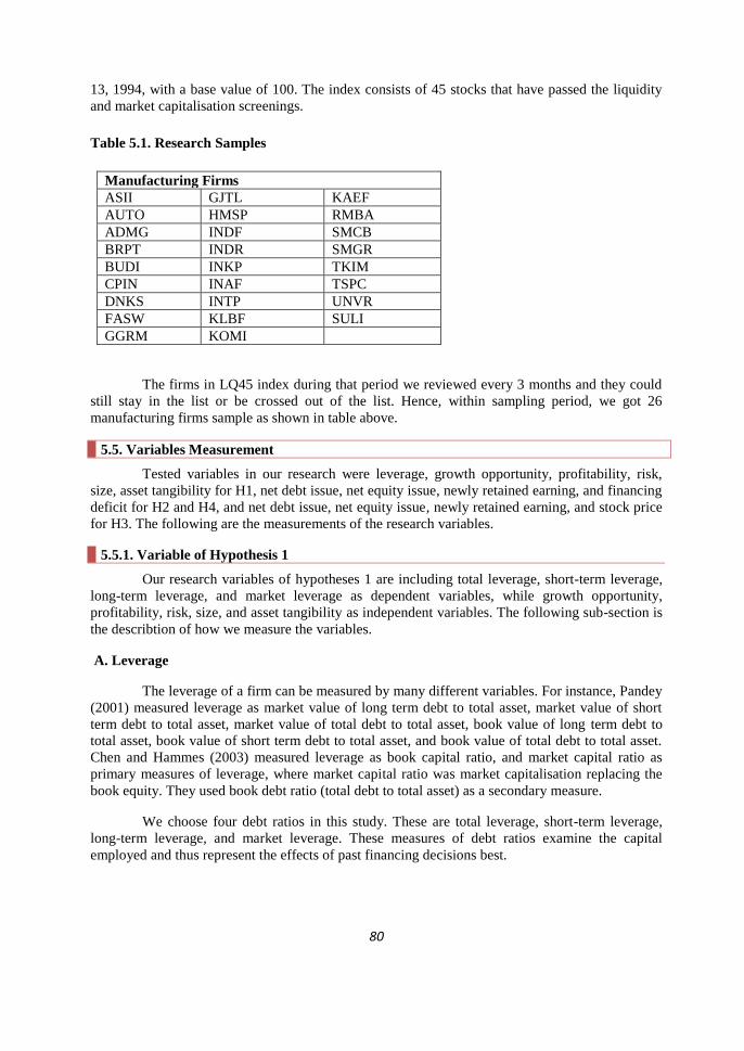
80
13, 1994, with a base value of 100. The index consists of 45 stocks that have passed the liquidity
and market capitalisation screenings.
Table 5.1. Research Samples
Manufacturing Firms
ASII GJTL KAEF
AUTO HMSP RMBA
ADMG INDF SMCB
BRPT INDR SMGR
BUDI INKP TKIM
CPIN INAF TSPC
DNKS INTP UNVR
FASW KLBF SULI
GGRM KOMI
The firms in LQ45 index during that period we reviewed every 3 months and they could
still stay in the list or be crossed out of the list. Hence, within sampling period, we got 26
manufacturing firms sample as shown in table above.
5.5. Variables Measurement
Tested variables in our research were leverage, growth opportunity, profitability, risk,
size, asset tangibility for H1, net debt issue, net equity issue, newly retained earning, and financing
deficit for H2 and H4, and net debt issue, net equity issue, newly retained earning, and stock price
for H3. The following are the measurements of the research variables.
5.5.1. Variable of Hypothesis 1
Our research variables of hypotheses 1 are including total leverage, short-term leverage,
long-term leverage, and market leverage as dependent variables, while growth opportunity,
profitability, risk, size, and asset tangibility as independent variables. The following sub-section is
the describtion of how we measure the variables.
A. Leverage
The leverage of a firm can be measured by many different variables. For instance, Pandey
(2001) measured leverage as market value of long term debt to total asset, market value of short
term debt to total asset, market value of total debt to total asset, book value of long term debt to
total asset, book value of short term debt to total asset, and book value of total debt to total asset.
Chen and Hammes (2003) measured leverage as book capital ratio, and market capital ratio as
primary measures of leverage, where market capital ratio was market capitalisation replacing the
book equity. They used book debt ratio (total debt to total asset) as a secondary measure.
We choose four debt ratios in this study. These are total leverage, short-term leverage,
long-term leverage, and market leverage. These measures of debt ratios examine the capital
employed and thus represent the effects of past financing decisions best.

81
Our measurement of book leverage is as measured by Rajan and Zingales (1995), Leary
and Roberts (2005), and Sbeiti (2010), and of market leverage is as measured by Bulan and Yan
(2009).
TLV=TD/TA
MRL = (TLV) / (TA+MV of Equity-TE)
Where TLV is total leverage, MRL is market leverage, TA is total asset, MV of equity is market
value of equity, and TE is total equity.
B. Growth Opportunities
The growth potential of a firm can be measured by many different variables. Rajan and
Zingales (1995) measured growth as Tobin‟s Q, Laarni Bulan and Zhipeng Yan (2009) measured
growth as market-to-book ratio as market equity/book equity, and Akhtar and Oliver (2006)
defined it as the average percentage change in total assets over the previous four years.
Chen and Hammes (2003), Leary and Roberts (2005), and Sbeiti (2010) measured growth
opportunities as the ratio of market value of assets (book value of assets plus market value of
equity less book value of equity) to book value of assets.
We measure growth opportunities as:
Growth = the ratio of market value of assets (book value of assets plus market value of
equity less book value of equity) to book value of assets.
C. Profitability
Profitability plays an important role in leverage decisions. Profitability is proxied by
return on assets. ROA represents the contribution of the firm‟s assets on profitability creation.
Profitability is a measure of earning power of a firm. The earning power of a firm is generally the
basic concern of its shareholders.
Akhtar and Oliver (2006) measured profitability as the average net income to total sales
for the past four years. Wafaa Sbeiti (2010) measured profitability as the ratio of operating profit
to book value of total assets. Titman and Wessels (1988), Drobetz and Fix (2003) measured it as
the ratio of operating income over total assets (ROA) and the ratio of operating income over sales.
Chen and Hammes (2003), Rajan and Zingales (1995), Abimbola Adedeji, Francisco
Sogorb-Mira y José López-Gracia (2003) measured profitability as earnings before interest and
taxes divided by total asset.
We measure profitability as:
Profitability = earnings before interest and taxes divided by total asset.
D. Risk
Earnings volatility measures the variability of the firm's cash flows as a proxy for the
costs of monitoring managers and of the risk of an insider's position. The use of longer time
periods causes a significant loss of the sample size.

82
Several measures of volatility were used in different studies, such as Bradley, Jarrell and
Kim (1984), Drobetz and Fix (2003) used variability as the standard deviation of the first
difference in annual earnings, scaled by the average value of the firm‟s total assets over time,
Booth et al. , (2001) the standard deviation of the return on sales.
Leary and Roberts (2005) measured cash flow volatility as the standard deviation of
earnings before interest and taxes, however they were based on (up to) the previous 10 years of
data for a given firm-year observation while we were up to the previous 3 years of data for a given
firm-year observation.
Risk = coefficient of variation in earnings before interest and taxes (EBIT) over three years.
E. Size
Firm size provides a measure of the agency costs of equity and the demand for risk
sharing. Firm size is likely to capture other firm characteristics as well (e.g., their reputation in
debt markets or the extent their assets are diversified).
Titman and Wessels (1988) and Drobetz and Fix (2003) measured firm size as the natural
logarithm of net sales. Chen and Hammes (2003) measured firm size as in Rajan and Zingales
(1995) that is the natural logarithm of total turnover.
Akhtar and Oliver (2006), Leary and Roberts (2005), Francisco Sogorb-Mira y José López-Gracia
(2003), and Sbeiti (2010) measured size as the natural logarithm of total assets.
Size = the natural logarithm of total assets.
F. Tangibility
The tangibility of assets represents the effect of the collateral value of assets of the firm‟s
gearing level. There are various conceptions for the effect of tangibility on leverage decisions. If
debt can be secured against assets, the borrower is restricted to using debt funds for specific
projects. Creditors have an improved guarantee of repayment, but without collateralised assets,
such a guarantee does not exist.
Leary and Roberts (2005), Bulan and Yan (2009) measured tangibility as net property,
plant and equipment divided by total assets. Huang and Song, Drobetz and Fix (2003), Abimbola
Adedeji, Dilek Teker,Ozlem Tasseven, and Ayca Tukel (2009) measured tangibility as fixed assets
divided by total assets.
Tangibility = fixed assets divided by total assets.
5.5.2 Measuring Variables of Hypotheses 2, 3, and 4
A. Financing Deficits
Bharath, Pasquariello, and Wu (2008) measure firms‟ financing deficits, dividends,
investments, and cash flow separately. Frank and Goyal (2003) measure deficit as dividend plus
investment and cashflow. Meanwhile, investment measured as capital expenditure and working
capital to capture a firm‟s demand for funds due to its real investments. Bulan and Yan (2009)
measure deficit as the financing deficit in period t scaled by total assets at the beginning of period
t, financing deficit as net equity plus net debt issues, and capital expenditures as capital
83
expenditures divided by total assets. Frank and Goyal (2007) measure the deficit as cash dividends
plus investments plus change in working capital minus internal cash flow.
Sogorb-Mira and López-Gracia measured the financing deficit would be as ∆ Fixed
current investment as the sum of capital expenditures, increase in investments, acquisitions, and
other use of funds, less sale of plant, property, and equpment and sale of investment. Cash flow
defined as cash flow after interest and taxes net of dividends, respectively.
Financing Deficit = DIV + CAPEX + LTD payment + Δ WC – CF
in which DIV is dividend payments, CAPEX is capital expenditures, ΔWC is the net change in
working capital, and CF is operating cash flow (after interest and taxes), long-term debt payment.
All variables are scaled by total assets, as in Frank and Goyal (2003).
B. Net Debt Issue
Leary and Roberts (2005) measure debt issuances as a change in total debt (long term
plus short term) divided by total assets in an excess of 5%. Frank and Goyal (2007) net debt issued
as long-term debt issuance minus long-term debt redemption. Bulan and Yan (2009) measure net
debt issued scaled by total assets, or net debt [long-term debt issuance minus long-term debt
reduction divided by total assets.
Net debt issue = (dTA/TA) - (Net equity issue) – (dRE/TA)
Where TA is total asset, dTA is change in total asset, and dRE is change in retained earning.
C. Net Equity Issue
Leary and Roberts (2005) measured equity issuances for year t as sale of common and
preferred stock net of purchase of common and preferred stock. Frank and Goyal (2007) measured
net equity issued as the issue of stock minus the repurchase of stock. Bulan and Yan (2009)
measured net equity as sale of common and preferred stock minus purchase of common and
preferred stock divided by total assets..
Net equity issue = (dEq/TA) - (dRE/TA), and
NRE = dRE/TA
Where TA is total asset, dEq is change in book equity, NRE is newly retained earning, and dRE is
change in retained earning.
5.6. Hypotheses Testing
We have tested hypotheses 1-4 using regression. We used this statistical technique as we
explored linear relationships between the predictor and criterion variables. The criterion variable
and the predictor variable we used for making a prediction should be measured on a continuous
scale (ratio scale). We also tested H2 by using an augmented model.

84
5.6.1. Hypothesis 1
The objective of testing hypothesis 1 is to examine the influence of growth opportunity,
profitability, risk, size, and asset tangibility on short-term leverage, long-term leverage, total
leverage, and market leverage.
The regression equation for hypotheses 1a, 1b, 1c, 1d, 1e, 1f, is as follows:
Y = a + β1 * X1 + β2 * X2 + β3 * X3 + β4 * X4 + β5 * X5 + e
Where:
Y = is the value of the dependent variable, Debt ratio
a = is the intercept of the regression line on the Y axis when X= 0
β = is the slope of the regression line
X1 = Growth opportunity
X2 = Profitability
X3 = Risk
X4 = Size
X5 = Asset tangibility
5.6.2. Hypothesis 2
The objective of testing hypothesis 2 is to examine how firms in the manufacturing sector
raise capital for investments externally (with debt, equity, or debt to repurchase equity).
Hypothesis 2 was analysed by using the mixed method approach.
A. Quantitative Analysis
For testing hypothesis 2, the independent variable was financing deficit, and net debt
issue, net equity issue, and net debt issue to repurchase equity were the dependent variables.
Therefore, the steps to analyse the relationship between variables are as follows:
A.1. Measuring the Financing Deficit/Surplus
The financing deficit would be approximated as:
FINANCING DEFICIT = DIV + CAPEX + ΔWC + LTD payment − CF
In which DIV is dividend payments, CAPEX is capital expenditures, ΔWC is the net change in
working capital, and CF is operating cash flow (after interest and taxes), LTD payment is long-
term debt payment. All variables are scaled by total assets, as in Frank and Goyal (2003).
A positive value of financing deficit indicates a financing deficit and a negative one
indicates financing surplus. The financing deficit/surplus in equation is equivalent to the one used
in previous studies.
85
A.2. Testing the Pecking Order Theory
In Bulan and Yan (2007), the pecking order theory of Myers and Majluf (1984) and
Myers (1984)) and its extensions (Lucas and McDonald (1990)) is based on the idea of
asymmetric information between managers and investors. Managers know more about the true
value of the firm and the firm‟s riskiness than less informed outside investors. If the information
asymmetry causes the underpricing of the firm‟s equity and the firm is required to finance a new
project by issuing equity, the underpricing may be so severe that new investors accept the largest
part of the net present value of the project, resulting in a net loss to existing shareholders. Thus,
managers who work in the greatest interest of the current shareholders will reject the project. To
avoid the underinvestment problem, managers will search for financing the new project using a
security that is not undervalued in the market, such as internal funds.
Consequently, this affects the choice between internal and external financing. The
pecking order theory is capable to explain why firms tend to depend on internal sources of funds
and prefer debt to equity if external financing is required. Thus, a firm‟s leverage is simply the
cumulative results of the firm‟s attempts to mitigate information asymmetry. Due to the valuation
discount that less-informed investors apply to newly issued securities, so firms choose internal
funds first, then debt and equity last to satisfy their financing needs (Bulan and Yan, 2007).
In this section, we implement a test of the pecking order theory proposed by Shyam-
Sunder and Myers (1999) given by the following:
Net Debt Issue = a + b1 * Deficit + ε
Where net debt issued and financing deficit, i.e. uses of funds minus internal sources of funds,
(both scaled by total assets). This deficit is financed with debt and/or equity. If firms are consistent
with the pecking order, changes in debt should track changes in the deficit one-for-one. Hence, the
expected coefficient on the deficit is 1. Frank and Goyal (2003) showed that this test performed
poorly for small firms and performed best for large firms. However, since small firms were
thought to suffer most from asymmetric information problems, hence they should be the ones
following the pecking order.
A.3. Testing the Pecking Order and Debt Capacity with an Augmented Model
In Laarni Bulan Zhipeng Yan (2007, as an alternative means of accounting for a firm‟s
debt capacity, Lemmon and Zender (2007) and Agca and Mozumdar (2004) augmented equation
with the deficit-squared:
Net Debt Issue = a + b1 * Deficit + b2 * Deficit2 + ε
To estimate equation, we follow Bulan and Yan (2009). Firms that in accordance with the
pecking order more strongly should have a debt-deficit sensitivity that is closer to one. The
quadratic specification was used to account for requiring debt capacity constraints. This deficit is
financed with debt and/or equity. If firms follow the pecking order, variations in debt should
follow changes in the deficit one-for-one (Shyam-Sunder and Myers, 1999). If firms are financing
their deficit with debt first and issue equity only when they achieve their debt capacities, then net
debt issued is a concave function of the deficit (Chirinko and Singha, 2000) and the coefficient on
the squared deficit term would be negative. The larger the deficit, the more probably it is for a firm
to attain its debt capacity. In these instances, the debt-deficit sensitivity should be lower. A
negative coefficient on the squared deficit term implies that firms are limited by their debt capacity
inadequacy and they have to choice to issuing equity. A squared deficit coefficient that is large in

86
absolute value describes a greater reliance on equity finance for larger values of the financing
deficit. If firms are issuing equity first and debt is the residual source of financing, then this
relationship should be convex and the coefficient on the squared deficit term would be positive. If
debt and equity are issued in static proportions, the deficit would have no influence on net debt
issued.
B. Qualitative Analysis
To make sure that our regression result is robust, we also analyse the results qualitatively
by using graphics and table analysis.
5.6.3. Hypothesis 3
The objective of testing H3 is to test the effect of issuing net debt, issuing net equity, and
issuing net debt to repurchase equity, on the firm‟s stock price. The regression equation for
hypothesis 3a, 3b, and 3c are as follow:
Y1 = a + β1 * X1 + e
Y2 = a + β2 * X2 + e
Y3 = a + β3 * X3 + e
Where:
Y = stock price
X1 = net debt issue
X2 = net equity issue
X3 = debt issue to repurchase equity
a = is the intercept of the regression line on the Y axis when X=0
β = is the slope of the regression line
5.6.4. Hypothesis 4
The objective of testing hypothesis 4 is to examine the firm‟s capital structure over the
life cycle of the firm to solve the problem of firm financing deficit. In testing the hypothesis, we
first classified firms into two cohorts according to their life cycle stage, namely, firms in their
growth stage and firms in their mature stage. Then we classified firms into small firms and large
firms, and additionally young firms and old firms.
Since we would like to examine how growth-mature firms and small-large firms finance
their deficit, hence, it is important to make sub distinctions in the theoretical framework between
growth-mature firms and small-large firms. Maturity and size can be regarded as a proxy for
information asymmetry between firm insiders and the capital markets. Mature [large] firms are
more closely observed by analysts and should therefore be more capable of issuing more equity,
and have lower debt (e.g., their reputation in debt markets or the extent their assets are diversified).
Growth [small] firms are on the other hand. Therefore, it is important to make sub distinctions in
the theoretical framework between growth-mature firms and small-large firms.
87
In the context of a firm‟s life cycle, we expected that asymmetric information problems
were more severe among growth [small] firms compared to firms that have reached maturity.
Hence, the theory predicts that fast-growing [smaller] firms should be following the pecking order
more closely.
Life Cycle Definition
Bulan and Yan (2009) defined the growth stage as the first six-year period after the year
of the firm‟s initial public offering (IPO). This definition may not necessarily apply to some firms
from a mechanical point of view. However, the IPO itself is an important financing decision that a
firm has to make. Here, Bulan and Yan (2009) treated the IPO as the starting point of the growth
stage (or the “new growth” stage).
DeAngelo, DeAngelo and Stulz (2006), among others, found that a firm‟s propensity to
pay dividends was a function of the stage where the firm is in its life cycle. In particular, Bulan,
Subramanian and Tanlu (2007) found that dividend initiators were mature firms. Based on this
body of work, they identified firms in their mature stage by their dividend initiation history. First,
they used the entire compustat industrial annual database to find consecutive six-year periods for
which a firm has positive dividends. They required that such a period should immediately follow
at least one year with zero or missing dividends. They considered these 6-year dividend payment
periods as the mature stage of a firm‟s life cycle.
1. Growth Firms and Mature Firms
We took Grullon, Michaely and Swaminathan (2000), DeAngelo, DeAngelo and Stulz
(2005) and Bulan, Subramanian and Tanlu as the references (2007) who found that firms initiated
dividends were mature firms. Thus, we identified firms in their mature stage by their dividend
history. Halov and Heider (2005), Leary and Roberts (2006) and Byoun (2007) showed that firm
financing choice was complex and was driven by many factors which included both pecking order
and trade-off theory considerations.
We constructed two samples of firms according to their life cycle stage: firms in their
growth stage and firms in their mature stage. Bulan and Yan (2007) set the length of each stage to
be 6 years. Evans (1987) defined six years old or younger as young firms and seven years or older
as old firms. We followed Bulan and Yan (2007) to set the length of each stage to be 6 years.
Growth Stage
Our sample was constructed from the manufacturing sector of the LQ45 index over the
1994- 2007 period. Some previous research defined the growth stage to be the first six-year period
after the year of the firm‟s IPO, however we defined the growth stage to be the firms that paid
dividend less then 5 years sequencialy.
Mature Stage
Bulan, Subramanian and Tanlu (2007) found that firms initiated dividends are mature
firms. Thus Bulan and Yan (2007) identified firms in their mature stage by their dividend history.
We took Bulan and Yan (2007) as a reference to construct the sample as follows: we included the
former 6-year period in our sample. This 10-year requirement was to ensure that whatever reason
for the dividend omission, the firm had fully recovered and re-emerged as a regular dividend
payer. We consider these 6-year dividends payment periods as the mature stage of a firm‟s life

88
cycle. We found that 10 firms had one 6-year dividend payment period; while 16 firms had less
than one 6-year dividend payment periods among the 26 firms.
Table 5.2. Growth Firms
No. Firm Life Cycle
1 ADMG Growth
2 BRPT Growth
3 BUDI Growth
4 CPIN Growth
5 DNKS Growth
6 FASW Growth
7 GJTL Growth
8 INDR Growth
9 INKP Growth
10 INAF Growth
11 INTP Growth
12 KOMI Growth
13 SMCB Growth
14 TKIM Growth
15 TSPC Growth
16 SULI Growth
Table 5.3. Mature Firms
No. Firm Life Cycle
1 ASII Mature
2 AUTO Mature
3 GGRM Mature
4 HMSP Mature
5 INDF Mature
6 KAEF Mature
7 KLBF Mature
8 RMBA Mature
9 SMGR Mature
10 UNVR Mature
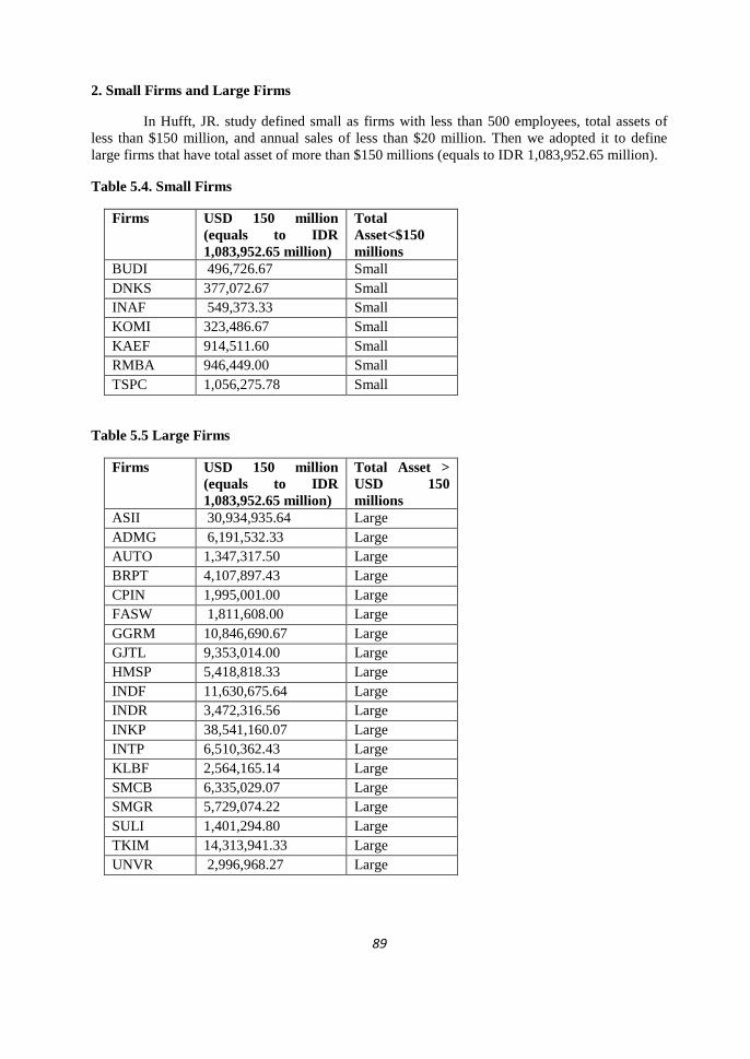
89
2. Small Firms and Large Firms
In Hufft, JR. study defined small as firms with less than 500 employees, total assets of
less than $150 million, and annual sales of less than $20 million. Then we adopted it to define
large firms that have total asset of more than $150 millions (equals to IDR 1,083,952.65 million).
Table 5.4. Small Firms
Firms USD 150 million
(equals to IDR
1,083,952.65 million)
Total
Asset<$150
millions
BUDI 496,726.67 Small
DNKS 377,072.67 Small
INAF 549,373.33 Small
KOMI 323,486.67 Small
KAEF 914,511.60 Small
RMBA 946,449.00 Small
TSPC 1,056,275.78 Small
Table 5.5 Large Firms
Firms USD 150 million
(equals to IDR
1,083,952.65 million)
Total Asset >
USD 150
millions
ASII 30,934,935.64 Large
ADMG 6,191,532.33 Large
AUTO 1,347,317.50 Large
BRPT 4,107,897.43 Large
CPIN 1,995,001.00 Large
FASW 1,811,608.00 Large
GGRM 10,846,690.67 Large
GJTL 9,353,014.00 Large
HMSP 5,418,818.33 Large
INDF 11,630,675.64 Large
INDR 3,472,316.56 Large
INKP 38,541,160.07 Large
INTP 6,510,362.43 Large
KLBF 2,564,165.14 Large
SMCB 6,335,029.07 Large
SMGR 5,729,074.22 Large
SULI 1,401,294.80 Large
TKIM 14,313,941.33 Large
UNVR 2,996,968.27 Large

90
3. Young Firms and Old Firms
Evans (1987) defined six years old firms or younger as young firms and seven years firms
or older as old firms. We followed this study and set the length of each stage to be 7 years
(however, this restriction is not true for some firms from a manufacturing point of view). To take
an example, KAEF was founded in 1969 and went public also in 2001. This firm is “old” enough
and is mature in many respects. However, the IPO itself is an important financing decision that a
firm has to make, and in many cases, indicates a significant change in the firm‟s development over
its life cycle. Here, we treated the IPO as an important turning point in a firm‟s history and as the
starting point of the old/young stage. Table showed that INAF and KAEF are 6 years from listing
date to 2007 as our sampling period from 1994 to 2007.
Table 5.6. Young and Old Firms
Established Listed How Old Listed in IDX (no.
of years from
listed to 2007)
ASII 20 Feb 1957 04 Apr 1990 50 17
AUTO 04 Apr 1979 01 Okt 1993 28 14
ADMG 25-Apr-1986 20-Oct-1993 21 14
BRPT 04-Apr-1979 01-Oct-1993 28 14
BUDI 15-Jan-1979 08-May-1995 28 12
CPIN 07 Jan 1972 18 Mar 1991 35 16
DNKS 25-Mar-1974 13-11-1989 33 18
FASW 13-Jun 87 19-Dec 1994 20 13
GGRM 26-Jun 1958 27-Aug 1990 49 17
GJTL 24-Aug 1951 08-May 1990 56 17
HMSP 27-Mar-1905 15-Aug-1990 102 17
INDF 14-Aug-1990 14-Jul-1994 17 13
INDR 03-Apr-1974 03-Aug-1990 33 17
INKP 07-Dec-1976 16-Jul-1990 31 17
INAF 02-Jan-1996 17-Apr-2001 11 6
INTP 16 Jan 1985 05 Des 1989 22 18
KLBF 10-Sep-1966 30-Jul-1991 41 16
KOMI 13-Dec-1982 31-Oct-1995 25 12
KAEF 23-Jan-1969 04-Jul-2001 38 6
RMBA 19-Jan-1979 05-Mar-1990 28 17
SMCB 15-Jun-1971 10-Aug-1977 36 30
SMGR 25-Mar-1953 08-Jul-1991 54 16
TKIM 02-Oct-1972 03-Apr-1990 35 17
TSPC 20-May-1970 17-Jun-1994 37 13
UNVR 05-Dec-1933 11-Jan-1982 74 25
SULI 14-Apr-1980 21-Mar-1994 27 13

91
As the equations applied in hypothesis 2, we also tested hypothesis 4 by following a test
of the pecking order theory proposed by Shyam-Sunder and Myers (1999) over the life cycle of the
firm.
5.7. Regression Analysis
Our regression analysis consists of the un-standardised Beta coefficients, the standardised
Beta coefficients, analysis of variance (ANOVA), coefficients of determination (R2), descriptive
statistics, and regression assumptions of hypotheses 1-4.
A. The Un-standardised Beta Coefficients
The Un-standardised Beta Coefficients (B) is the value for the regression equation for
predicting the dependent variable from the independent variable. These are called un-standardised
coefficients because they are measured in their natural units. As such, the coefficients cannot be
compared with one another to determine which one is more influential in the model, because they
can be measured on different scales.
B. The Standardised Beta Coefficients
The Standardised Beta coefficients give a measure of the contribution of each variable to
the model. A large value indicates that a unit change in this predictor variable has a large effect on
the criterion variable. The t and sig (p) values give a rough indication of the impact of each
predictor variable a big absolute t value and small p value suggests that a predictor variable is
having a large impact on the criterion variable.
When we have only one predictor variable in our model, then beta is equivalent to the
correlation coefficient between the predictor and the criterion variable. This equivalence makes
sense, as this situation is a correlation between two variables.
C. Analysis of Variance (ANOVA)
Analysis of variance enables an extrapolation of the t test results of two groups to three or
more groups. The F-statistic will be calculated for analysis of variance (ANOVA) to test whether
group population means are all equal or not. When the F-statistic is found significant, we may
conclude that at least one of the population means of the groups differs from the others, but
ANOVA does not tell us which groups are different from which. If this is the case, a multiple-
comparison analysis by pairwise group comparison will be an appropriate answer to this question
(Bekiro, 2001).
The statistical significance as depicted in the ANOVA analysis of the models for firms
reach statistical significance at significance value of p<0.05 (Coakes and Steed, 2003; and Pallant,
2005).
D. The Coefficient of Determination (R2)
The multiple correlation coefficients (R) are the linear correlation between the model-
predicted and the observed values of the dependent variable. The coefficient of determination, or
simply R-squared, has its value always between 0 and 1, and is interpreted as the percentage of
variation of the response variables explained by the regression line. If there is no linear relation
between the dependent and independent variable, R2
is 0 or very small. If all the observations fall
on the regression line, R2
is 1. This measure of the goodness of fit of a linear model is also called
the coefficient of determination. The sample estimate of R2
tends to be an optimistic estimate of

92
the population value. Adjusted R Square is designed to more closely reflect how well the model
fits the population and is usually of interest for models with more than one predictor.
A high value of R2, suggesting that the regression model explains the variation in the
dependent variable well, is obviously important if one wishes to use the model for predictive or
forecasting purposes. To be sure, a large unexplained variation in the dependent variable will
increase the standard error of the coefficients in the model (which are a function of the estimated
variance of the noise term), and hence regressions with low values of R2 will often (but by no
means always) yield parameter estimates with small t-statistics for any null hypothesis. Because
this consequence of a low R2 will be reflected in the t-statistics, however, it does not afford any
reason to be concerned about a low R2 per se. R Square (R
2) is the square of the measure of
correlation and indicates the proportion of the variance in the criterion variable which is accounted
for by our model.
E. Descriptive Statistics
Descriptive statistics describe the value of each variable including mean, minimum, and
maximum values.
F. Regression Assumptions of Hypothesis 1-4
Before analyzing regression coefficients of variables, we must first make several
assumptions about the population of the research. They represent an idealisation of reality, and as
such, they are never likely to be entirely satisfied for the population in any real study (Van Horne,
1998). A good regression model should not have the following assumptions:
1. Multicollinearity
Multicollinearity implies that for some set of explanatory variables, there is an exact
linear relationship in the population between the means of the response variable and the values of
the explanatory variables (Van Horne, 1998). The goal of the multicollinearity test is to analyse
whether there is correlation between independent variables.
Multicollinearity in the regression model can be detected such as by testing the R2 value
and/or analysing the correlation matrix (Ghozali, 2002). The other ways to detect the problem of
multicollinearity are the tolerance values and VIF (Hair et al., 1998).
Correlations between Variables
For correlations between variables, we do not want strong correlations between the
criterion and the predictor variables.
The Tolerance and VIF
The tolerance values are a measure of the correlation between the predictor variables and
can vary between 0 and 1. The closer to zero the tolerance value is for a variable, the stronger the
relationship between this and the other predictor variables. We should worry about variables that
have a very low tolerance (Van Horne, 1998). SPSS will not include a predictor variable in a
model if it has a tolerance of less that 0.0001. However, we may want to set your own criteria
rather higher – perhaps excluding any variable that has a tolerance level of less than 0.01.
Meanwhile, VIF is an alternative measure of collinearity (in fact it is the reciprocal of
tolerance) in which a large value indicates a strong relationship between predictor variables.

93
2. Autocorrelation
Autocorrelation requires probabilistic independence of the errors. This assumption means
that information on some of the errors provides no information on other errors. For time series data
this assumption is often violated. This is because of a property called autocorrelation (Van Horne,
1998).
Test of autocorrelation aims to examine whether in a linear regression model has
correlation between trouble errors in the period t with an error in the period t-1 (before). One of
the methods that can be used to detect autocorrelation is the Durbin Watson (DW). DW value
shows that there is no autocorrelation in regression model.
Durbin Watson (DW) Test Statistic
In Field (2008), Durbin Watson test statistic, a test for correlation between errors.
Specifically, it tests whether adjacent residuals are correlated. In short, this option is important for
testing whether the assumption of independent errors is tenable. The test statistic can vary between
0 and 4 with a value of 2 meaning that the residuals are uncorrelated. A value greater than 2
indicates a negative correlation between adjacent residuals whereas a value below 2 indicates a
positive correlation. The size of the DW statistic depends upon the number of predictors in the
model, and the number of observations. As a conservative rule of thumb, Field (2009) suggested
that, values less than 1 or greater than 3 gave definitely cause for concern, however values closer
to 2 may still be problematic depending on the sample and model.
3. Heteroscedasticity
This assumption concerns variation around the population regression line. Specifically, it
states that the variation of the Y‟s about the regression line is the same, regardless of the value of
the X‟s (Van Horne, 1998).
Test of heteroscedasticity aims to interpret whether the regression model has the
differences residual variance from one observation to another observation (Ghozali, 2002). If the
residual variance from one observation to another observation is the same, it is called
homoscedasticity.
The graphic of scatterplot (in appendix) shows that the dots have not established a
specific pattern. Some of the dots located adjacent but some other dots spread above and below the
numbers of 0 at the axis Y. Thus, the data in the graphics exhibits homoscedasticity.
4. Normally Distributed
The assumption states that the errors are normally distributed. We can check this by
forming a histogram of the residuals. If the assumption holds, then the histogram should be
approximately symmetric and bell-shaped. But if there is an obvious skewness, too many residual
more than, say, two standard deviations from the mean, or some other non-normal property, then
this indicates a violation of the assumption (Van Horne, 1998).
From the graphics of histogram and normal P-P plot (in appendix), we concluded that the
histogram gave the normal pattern of distribution. Meanwhile, the graphic of normal P-P plot
shows that the dots spread around the diagonal line, and the spreading follows the diagonal line.
Both graphics show that the data meets reasonable assumption of normality.

94
Based on the results of assumptions of population described above, the regression model
does not have the assumptions of heteroscedasticity, multicollinearity, autocorrelation, and the
data are normally distributed. Thus, our regression model is appropriate to use for testing the
hypothesis 1- 4.
5.8. The Credibility of Research Findings
Underpinning the above discussion on multi-method usage has been the issue of the
credibility of research findings. This is neatly expressed by Raimond (1993) and Rogers (1961,
cited by Raimond, 1993). Reducing the probability of getting the answer wrong means that
concentration has to paid to two particular emphases on research design, namely, reliability and
validity.
5.8.1 Reliability
Reliability examines whether the measurement can be repeated; that is, whether we are
measuring something that can be replicated over time instead of a random effect. Reliability can be
evaluated by using the following three questions (Easterby-Smith et al., 2002):
1. Will the measures yield the same results on other occasions?
2. Will similar observations be reached by other observers?
3. Is there transparency in how sense was made from the raw data?
To ensure that this research has answered these three questions, we have reviewed the previous
research findings concluded by other researchers from many research setting and time period.
5.8.2 Validity
Validity is concerned with whether the findings are really about what they illustrate to be
about. Is the relationship between two variables a causal relationship? We minimised the potential
lack of validity in the conclusions by analysing the results obtained quantitatively and
qualitatively. Even though analysing results obtained quantitatively and qualitatively does not
minimise the potential lack of validity, the results obtained should be consistent with each other.
5.8.3 Generalisability
Generalisability is sometimes referred to as external validity. A concern we may have in
the design of our research is the extent to which your research results are generalisable: that is,
whether our findings may be equally applicable to other research settings, such as other
organisations.
In this research, the purpose of our research will not be to produce a theory that is
generalisable to all populations. Our objective will be simply to try to explain what is happened in
Indonesia Capital Market. Therefore, our results can not be generalised.
5.9. The Limitations of Research Design
There is no research project without limitations; and there is no research as a perfectly
designed study. It is in line with Patton (1990), who noted that “there are no perfect research
designs and there are always trade-offs”. Yin (2003) also noted that limitations derived from the
conceptual framework and the study‟s design. Furthermore, each method, tool or technique has its
unique strengths and weaknesses (Smith, 1975).

95
Since all different methods will have different effects, it makes sense if we use different
methods to avoid the „method effect‟. It will lead us to greater confidence being placed in our
conclusions. Therefore, it is quite usual for a single study to combine quantitative and qualitative
methods and/or to use primary and secondary data. There are two major advantages to employ
multi-methods in the same study. First, different methods can be used for different purpose in a
study. The second advantage of applying multi-methods is that it enables triangulation to take
place. Triangulation refers to the use of different data collections methods within one study in
order to ensure that the data are telling us what we believe they are describing us.
In our research, we had two limitations as follow, the first is regarding to the limitation of
data, as sometimes the data are not complete. The second is regarding to the data analysis.
Therefore, we used regression and augmented equations and also qualitative analysis to explain the
finding of hypotheses.
96
6. PRESENTATION OF DATA AND ANALYSIS OF RESULTS
6.1 Research Question 1, Hypotheses, Hypotheses Testing, and Result Analysis
Chapter 6 described the hypothesis testing for research questions one and two, three, and
four, and discussed the results obtained in detail. The chapter discussed the results for each
research question.
In chapter 1, four research questions were introduced. A total of 4 major hypotheses were
constructed to assist in answering the research questions. Chapters 6 now discuss the findings from
this inquiry. It presented and discussed the results of testing hypotheses 1, 2, 3, and 4 that
belonged to research question one, two, three, and four respectively. The remaining research
questions, the associated hypotheses and the results are presented below.
6.1.1. Research Question 1
In this research, our minor research questions are as follow:
What are the determinants of capital structure of the firms in the manufacturing sector in
Indonesia?
a. As implied by the trade-off theory and the pecking order theory, do growth
opportunities have a positive relationship with debt ratio?
b. As the pecking order hypothesis, does a firm‟s profitability have a negative
relationship with level of debt? And as implied by the trade-off theory, does a firm‟s
profitability have a positive relationship with the debt ratio?
c. In accordance with the pecking order theory and trade-off theory, is there a negative
relationship between risk (earnings volatility) and debt ratio?
d. As suggested by the trade-off theory, does size has a positive relationship with debt
ratio? And as suggested by the pecking order theory of the capital structure, is there a
negative relationship between level of debt and size of the firm?
e. In accordance with the trade-off theory, is there a positive relationship between asset
tangibility and level of debt?
6.1.2. Hypothesis One (H1)
In this research, our minor hypotheses one (H1) are as follow:
H1.a: As implied by the trade-off theory and the pecking order theory, we hypothesise that growth
opportunity is positively related to debt ratios.
H1.b: As the pecking order hypothesis, we hypothesise that profitability has a negative
relationship with debt ratios and based on the trade-off theory we hypothesise that profitability has
a positive relationship with debt ratio.
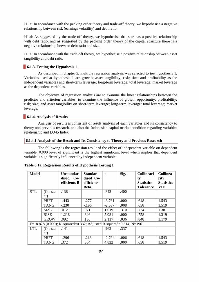
97
H1.c: In accordance with the pecking order theory and trade-off theory, we hypothesise a negative
relationship between risk (earnings volatility) and debt ratio.
H1.d: As suggested by the trade-off theory, we hypothesise that size has a positive relationship
with debt ratio, and as suggested by the pecking order theory of the capital structure there is a
negative relationship between debt ratio and size.
H1.e: In accordance with the trade-off theory, we hypothesise a positive relationship between asset
tangibility and debt ratio.
6.1.3. Testing the Hypothesis 1
As described in chapter 5, multiple regression analysis was selected to test hypothesis 1.
Variables used at hypothesis 1 are growth; asset tangibility; risk; size; and profitability as the
independent variables and short-term leverage; long-term leverage; total leverage; market leverage
as the dependent variables.
The objective of regression analysis are to examine the linear relationships between the
predictor and criterion variables, to examine the influence of growth opportunity; profitability;
risk; size; and asset tangibility on short-term leverage; long-term leverage; total leverage; market
leverage.
6.1.4. Analysis of Results
Analysis of results is consistent of result analysis of each variables and its consistency to
theory and previous research, and also the Indonesian capital market condition regarding variables
relationship and LQ45 Index.
6.1.4.1 Analysis of the Result and Its Consistency to Theory and Previous Research
The following is the regression result of the effect of independent variable on dependent
variable. 0.000 level of significant is the highest significant level which implies that dependent
variable is significantly influenced by independent variable.
Table 6.1a. Regression Results of Hypothesis Testing 1
Model Unstandar
dised Co-
efficients B
Standar
dised Co-
efficients
Beta
t Sig. Collineari
ty
Statistics
Tolerance
Collinea
rity
Statistics
VIF
STL (Consta
nt)
.138 .843 .400
PRFT -.443 -.277 -3.761 .000 .648 1.543
TANG -.230 -.196 -2.687 .008 .658 1.519
SIZE .012 .071 1.019 .310 .724 1.381
RISK 1.218 .346 5.081 .000 .758 1.319
GROW .092 .136 2.117 .036 .848 1.179
F=18.878 (0.000); R-squared=0.332; Adjusted R-squared=0.314; N=196
LTL (Consta
nt)
.141 .962 .337
PRFT -.296 -.213 -2.794 .006 .648 1.543
TANG .372 .364 4.822 .000 .658 1.519
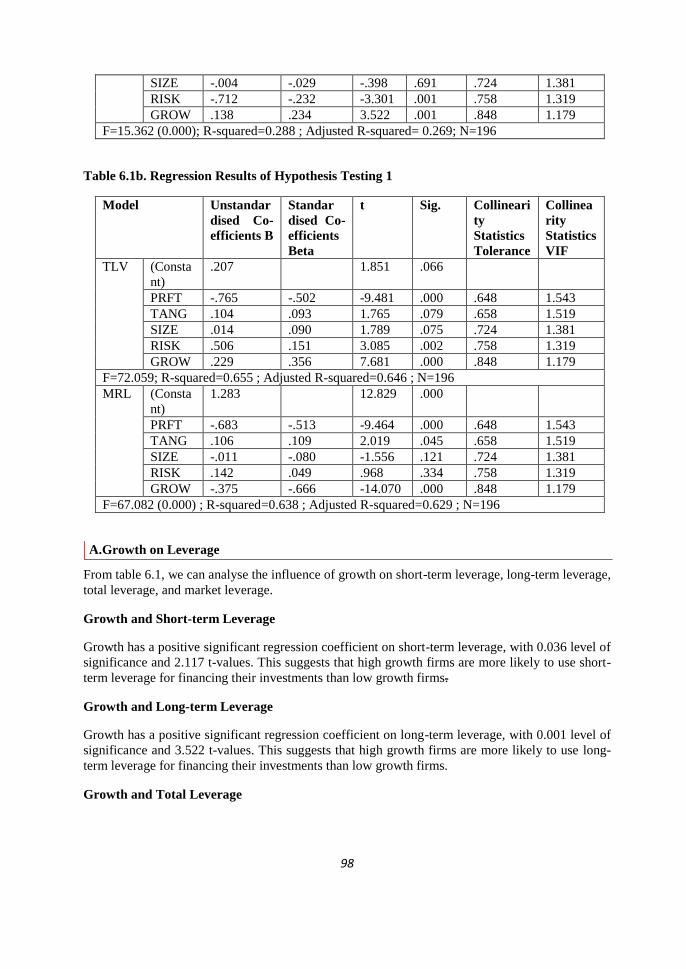
98
SIZE -.004 -.029 -.398 .691 .724 1.381
RISK -.712 -.232 -3.301 .001 .758 1.319
GROW .138 .234 3.522 .001 .848 1.179
F=15.362 (0.000); R-squared=0.288 ; Adjusted R-squared= 0.269; N=196
Table 6.1b. Regression Results of Hypothesis Testing 1
Model Unstandar
dised Co-
efficients B
Standar
dised Co-
efficients
Beta
t Sig. Collineari
ty
Statistics
Tolerance
Collinea
rity
Statistics
VIF
TLV (Consta
nt)
.207 1.851 .066
PRFT -.765 -.502 -9.481 .000 .648 1.543
TANG .104 .093 1.765 .079 .658 1.519
SIZE .014 .090 1.789 .075 .724 1.381
RISK .506 .151 3.085 .002 .758 1.319
GROW .229 .356 7.681 .000 .848 1.179
F=72.059; R-squared=0.655 ; Adjusted R-squared=0.646 ; N=196
MRL (Consta
nt)
1.283 12.829 .000
PRFT -.683 -.513 -9.464 .000 .648 1.543
TANG .106 .109 2.019 .045 .658 1.519
SIZE -.011 -.080 -1.556 .121 .724 1.381
RISK .142 .049 .968 .334 .758 1.319
GROW -.375 -.666 -14.070 .000 .848 1.179
F=67.082 (0.000) ; R-squared=0.638 ; Adjusted R-squared=0.629 ; N=196
A.Growth on Leverage
From table 6.1, we can analyse the influence of growth on short-term leverage, long-term leverage,
total leverage, and market leverage.
Growth and Short-term Leverage
Growth has a positive significant regression coefficient on short-term leverage, with 0.036 level of
significance and 2.117 t-values. This suggests that high growth firms are more likely to use short-
term leverage for financing their investments than low growth firms.
Growth and Long-term Leverage
Growth has a positive significant regression coefficient on long-term leverage, with 0.001 level of
significance and 3.522 t-values. This suggests that high growth firms are more likely to use long-
term leverage for financing their investments than low growth firms.
Growth and Total Leverage

99
Growth has a positive significant regression coefficient on total leverage, with 0.000 level of
significance and 7.681 t-values. This suggests that high growth firms are more likely to use total
leverage for financing their investments than low growth firms.
Growth and Market Leverage
Growth has a negative significant regression coefficient on market leverage, with 0.000 level of
significance and -14.070 t-values. This suggests that high growth firms are less likely to use
market leverage for financing their investments than low growth firms.
Our results showed that growth was positively related with short-term leverage, long-term
leverage, and total leverage. It was consistent with the pecking order theory. According to the
pecking order theory hypothesis, a firm will first use internally generated funds which may not be
sufficient for a growth firm. And the next option for the growth firms is to use debt financing
which implies that a growth firm will have a high leverage (Drobetz and Fix 2003).
Applying pecking order arguments, growth firms place a greater demand on the internally
generated funds of the firm. Consequentially, firms with relatively high growth will tend to issue
securities less subject to information asymmetries, i.e. short-term debt. This should lead firms with
relatively higher growth to having more leverage.
Our results were consistent with what Sogorb-Mira and Lopez-Gracia (2003) said that
there was a positive relation between growth and short-term leverage, long-term leverage, and
total leverage. Sogorb-Mira and López-Gracia (2003) tested leverage predictions of the trade-off
and pecking order models. They used panel data Spanish SMEs. Their result showed a positive
and statistically significant impact between growth opportunities and firm leverage. This result is
consistent with the Michaelas et al. (1999) argument, based on the idea that in SMEs the trade off
between independence and financing availability is more pronounced and the major part of debt
financing is short term.
Pandey (2001) examined the determinants of capital structure of Malaysian companies
and showed that growth variable had a positive significant influence on all types of book and
market value debt ratios. This finding supported both trade-off and pecking order theories. On the
other hand, according to Çağlayan and Şak (2010), market to book was found to have positive
effect on book leverage. Positive sign of market to book was also along the lines of pecking order
theory.
Our results were in line with what agency costs / trade-off theory that the growth was
negatively related with market leverage. Agency costs for growth firms are expected to be higher
as these firms have more flexibility with regard to future investments. The reason is that
bondholders fear that such firms may go for risky projects in future as they have more choice of
selection between risky and safe investment opportunities. Deeming their investments at risk in
future, bondholders will impose higher costs at lending to growth firms. Growth firms that are
facing higher cost of debt will use less debt and more equity. Congruent with this, Titman and
Wessels (1988), Barclay et al. (1995) and Rajan and Zingales (1995), all found a negative
relationship between growth opportunities and leverage.
Following the trade-off theory, for companies with growth opportunities, the use of debt
is limited as in the case of bankruptcy, the value of growth opportunities will be close to zero,
growth opportunities are particular case of intangible assets (Myers, 1984; Williamson, 1988 and
Harris and Raviv, 1990). Firms with less growth prospects should use debt because it has a
disciplinary role (Jensen, 1986; Stulz, 1990). Firms with growth opportunities may invest sub-
100
optimally, and therefore creditors will be more reluctant to lend for long horizons. This problem
can be solved by short-term financing (Titman and Wessels, 1988) or by convertible bonds (Jensen
and Meckling, 1976; Smith and Warner, 1979).
According to agency costs, on the other hand, Myers (1977) argued that due to agency
problems, firms invested in assets that might generate high growth opportunities in the future
faced difficulties in borrowing against such assets. For this reason, we might now instead expect a
negative relationship between growth and leverage.
Some research found the negative result, such as Huang and Song (2002), concluded that
the static trade-off model seemed better than the pecking order hypothesis in explaining the
features of capital structure for Chinese listed companies. They used sales growth rate to measure
the past growth experience and Tobin‟s Q to measure a firm‟s growth opportunity in the future.
Their finding showed that firms with a high growth rate in the past tended to have higher leverage,
while firms that had a good growth opportunity in the future (a higher Tobin‟s Q) tended to have
lower leverage.
Sbeiti (2010) found a negative relation between growth opportunities and leverage, it was
consistent with the predictions of the agency theory that high growth firms used less debt, since
they did not wish to be exposed to possible restrictions by lenders. However, variables such as
market to book ratio reflected the capital market valuation of the firm, which in turn was affected
by the conditions of the capital market.
In the Shah and Khan (2007) study, growth variable was significant and was negatively
related to leverage. As expected, this negative coefficient showed that growth firms did not use
debt financing. Their results were in conformity with the result of Titman and Wessels (1988);
Barclay, et al. (1995) and Rajan and Zingales (1995). The usual explanation was that growing
firms had more options of choosing between safe and risky firms.
In Gaud, Jani, Hoesli, and Bender (2003), the negative sign of growth confirmed the
hypothesis that firms with growth opportunities were less levered. To analyse further this
relationship, they observed a negative relationship between growth and leverage when market
values were used, and a positive relation when leverage was measured with book values.
B. Profitability on Leverage
We can see from table 6.1 to imply the influence of profitability on short-term leverage,
long-term leverage, total leverage, and market leverage.
Profitability and Short-term Leverage
Profitability has a negative significant regression coefficient on short-term leverage, with
0.000 level of significance and -3.761 t-values. This suggests that high profitability firms are less
likely to use short-term leverage for financing their investments than firms with low profitability.
High profitability firms in the manufacturing sector of the LQ45 Index are less likely to use short-
term leverage for financing their investments than low profitability firms.
Profitability and Long-term Leverage
Profitability has a negative significant regression coefficient on long-term leverage, with
0.006 level of significance and -2.794 t-values. This suggests that high profitability firms are less
likely to use long-term leverage for financing their investments than firms with low profitability.

101
Profitability and Total Leverage
Profitability has a negative significant regression coefficient on total leverage, with 0.000
level of significance and -9.481 t-values. This suggests that high profitability firms are less likely
to use total leverage for financing their investments than firms with low profitability.
Profitability and Market Leverage
Profitability has a negative significant regression coefficient on market leverage, with
0.000 level of significance and -9.464 t-values. This suggests that high profitability firms are less
likely to use market leverage for financing their investments than firms with low profitability.
Profitability has negative correlation with short-term leverage, long-term leverage, total
leverage, and market leverage. Comparing the results with the theory, all of our results are
negative and they are in line with the pecking order theory but contradicting with the trade-off
theory.
The pecking order theory, based on works by Myers and Majluf (1984) suggests that
firms have a pecking-order in the choice of financing their activities. Roughly, this theory states
that firms prefer internal funds rather than external funds. If external finance is required, the first
choice is to issue debt, then possibly with hybrid securities such as convertible bonds, then
eventually equity as a last resort (Brealey and Myers, 1991). This behaviour may be due to the
costs of issuing new equity, as a result of asymmetric information or transaction costs.
All things being equal, the more profitable the firms are, the more internal financing they
will have, and therefore we should expect a negative relationship between leverage and
profitability. This relationship is one of the most systematic findings in the empirical literature
(Harris and Raviv, 1991; Rajan and Zingales, 1995; Booth et al., 2001). There are conflicting
theoretical predictions on the effects of profitability on leverage (Rajan and Zingales, 1995); while
Myers and Majluf (1984) predicted a negative relationship according to the pecking order theory,
Jensen (1986) predicted a positive relationship. Following the pecking order theory, profitable
firms, which have access to retained profits, can use these for firm financing rather than accessing
outside sources.
However, in a trade-off theory framework, an opposite conclusion is expected. When
firms are profitable, they should prefer debt to benefit from the tax shield. In addition, if past
profitability is a good proxy for future profitability, profitable firms can borrow more as the
likelihood of paying back the loans is greater. From the trade-off theory point of view more
profitable firms are exposed to lower risks of bankruptcy and have greater incentive to employ
debt to exploit interest tax shields. Hence, high profitability firms in the manufacturing sector of
the LQ45 Index do not want to take benefit from the tax shield.
Meanwhile, based on agency theory, there are two possible explanations. Jensen (1986)
predicted a positive relationship between profitability and financial leverage, if the market for
corporate control was effective, such relation occurred because debt reduced the free cash flow
generated by profitability. However, if it was ineffective, Jensen (1986) predicted a negative
relationship between profitability and leverage.
Comparing the results with previous studies, they were consistent. Drobetz and Fix
(2003) tested leverage predictions of the trade-off and pecking order models using Swiss data.
Their results were in conformity with the pecking order model but contrary to the trade-off model,
more profitable firms used less leverage. They found that profitability was negatively correlated
102
with leverage, both for book and market leverage. This result reliably supported the predictions of
the pecking order theory.
The Huang and Song (2002) study results were consistent with the predictions of
theoretical studies and the results of previous empirical studies. Profitability was strongly
negatively related with total liabilities ratios. The Pandey (2001) results showed that profitability
had a significant inverse relation with all types of book and market value debt ratios. He showed
that the results confirmed findings of earlier studies and were consistent with pecking order theory
(Myers, 1984) that postulated a negative relationship between profitability and debt ratio.
Cole (2008) showed a consistent negative relation between profitability with the loan-to-
asset ratio. The coefficients for return on asset were significant. These later findings were strongly
supportive to the pecking order theory which predicted that profitable firms used less debt because
they could fund projects with retained earnings. It was inconsistent with trade-off theory that
predicted profitable firms used more debt to take advantage of the debt tax shield The other reason
was they had lower probability of financial distress.
Sbeiti (2010) found that firm profitability seemed to have a statistically negative and
significant relationship with both the book and market leverage in the three countries. It was
consistent with Booth et al. (2001), who reported the same results for the profitability variable and
argued that the importance of profitability was related to the significant agency and informational
asymmetry problems in developing countries. The results were also consistent with Titman and
Wessels (1988), Rajan and Zingales (1995), Cornelli et al. (1996), Bevan and Danbolt (2002) in
developed countries, Pandey (2001), Um (2001), Wiwattanakantang (1999), Chen (2004),
Deesomsak, Paudyal and Pescetto (2004) and Antoniou et al. (2007).
The Shah and Khan (2007) study found the negative sign and statistical significance.
Frydenberg (2001b) described retained earning as the most important source of financing. Good
profitability thus reduced the need for external debt. In Çağlayan and Şak (2010) study,
profitability was found to have negative effect on the book leverage. A negative relationship
between profitability and leverage was observed in the majority of empirical studies. This study
provided similar results confirming the pecking order theory rather than static trade-off theory.
In the Han-Suck Song (2005) study, profitability was negatively correlated with all three
leverage measures, which was in line with the pecking-order theory. Firms preferred using surplus
generated by profits to finance investments. This result might also indicate that firms in general
always preferred internal funds rather than external funds, irrespective of the characteristic of an
asset that should be financed (e.g. tangible or nontangible asset). Gaud, Jani, Hoesli and Bender
(2003), reported in several other studies that the profitability variable was negative and significant
in all cases (Rajan and Zingales, 1995; Booth et al., 2001; Frank and Goyal, 2002). This finding
provides support for the pecking order theory.
In Indonesia, previous empirical testing showed a significant negative relationship
between profitability and leverage. This phenomenon indicates that the lower the profitability, the
higher the leverage or vice versa. If the indication happens, it leads to a state that firm‟s debt to
help increasing liquidity but it is not supported by the firm‟s performance. This indicates the
occurrence of agency problems. If the opposite happens then the relationship is consistent with the
pot which states that profitability is negatively related to leverage. In this case the firm is the low
use of debt with high profitability. According to pecking order theory, high profitability firms
borrow less because such firms have more internal financing, while firms with lower profitability
require external funding and the consequence is debt accumulation (Sugiarto, 2009).

103
C. Risk on Leverage
The following result is the analysis of the effect of risk on short-term leverage, long-term
leverage, total leverage, and market leverage (table 6.1).
Risk and Short-term Leverage
Risk has a positive significant regression coefficient on short-term leverage, with 0.000
level of significance and 5.081 t-values. This suggests that high risk firms are more likely to use
short-term leverage for financing their investments than low risk firms.
Risk and Long-term Leverage
Risk has a negative significant regression coefficient on long-term leverage, with 0.001
level of significance and -3.301 t-values. This suggests that high risk firms are less likely to use
long-term leverage for financing their investments than low risk firms.
Risk and Total Leverage
Risk, has a positive significant regression coefficient on total leverage, with 0.002 level
of significance and 3.085 t-values. This suggests that high risk firms are more likely to use total
leverage for financing their investments than low risk firms.
Risk and Market Leverage
Risk has a positive but not significant regression coefficient on market leverage, with
0.334 level of significance and 0.968 t-values. This suggests that high risk firms are more likely to
use market leverage for financing their investments than low risk firms.
Our result showed that risk has positive influence on short-term leverage, total leverage,
and market leverage, while it has negative effect on long-term leverage. The negative result
supported both the trade-off theory that the more volatile cash flows the higher the probability of
default and the pecking order theory that issuing equity is more costly for firms with high volatile
cash flows. Our positive result supported the agency theory that the problem of underinvestment
decreased when the volatility of the firms returns increased, hence, firms use more leverage.
Bradley et al., (1984); Kester, (1986); Titman and Wessels (1988) found that since higher
variability in earnings indicates that the probability of bankruptcy increases, they expect that firms
with higher income variability have lower leverage. Firms that have high operating risk can lower
the volatility of the net profit by reducing the level of debt. A negative relation between operating
risk and leverage is also expected from a pecking order theory perspective: firms with high
volatility of results try to accumulate cash during good years, to avoid under-investment issues in
the future. Drobetz and Fix (2003) found as expected, the leverage was negatively related to the
volatility. They also showed that their finding supported both the trade-off theory (more volatile
cash flows increase the probability of default) and the pecking order theory (issuing equity is more
costly for firms with volatile cash flows).
Pandey (2001) found that there was a negative relation of earnings volatility with book
and market value long-term debt ratio, which was consistent with the trade-off theory. It also
revealed a positive relation between risk and short-term debt ratios.

104
We found that risk was positively related with the short-term leverage, and risk was also
positively related with the total leverage and market leverage. Those were in line with the agency
theory that Cools (1993) said it suggested positive relationship between earning volatility and
leverage. He said that the problem of underinvestment decreased when the volatility of the firms
return increased.
The Huang and Song (2002) results showed that there was a positive relation between
total liabilities ratio and volatility. It was consistent with Hsia‟s (1981) view that firms with a
higher leverage level tended to make riskier investment. They found that the companies with high
leverage in China tended to make riskier investments.
D. Size on Leverage
Table 6.1 indicates the regression result of the effect of size on short-term leverage, long-
term leverage, total leverage, and market leverage. Our analysis is as follows:
Size and Short-term Leverage
Size has a positive but not significant regression coefficient on short-term leverage, with
0.310 level of significance and 1.019 t-values. This suggests that larger firms are more likely to
use short-term leverage for financing their investments than small size firms.
Size and Long-term Leverage
Size has a negative but not significant regression coefficient on long-term leverage, with
0.691 level of significance and -0.398 t-values. This suggests that larger size firms are less likely
to use long-term leverage for financing their investments than small size firms.
Size and Total Leverage
Size has a positive but not significant regression coefficient on total leverage, with 0.075
level of significance and 1.789 t-values. This suggests that larger size firms are more likely to use
total leverage for financing their investments than small size firms.
Size and Market Leverage
Size has a negative significant regression coefficient on market leverage, with 0.121 level
of significance and -1.556 t-values. This suggests that larger size firms are less likely to use market
leverage for financing their investments than small size firms.
Our results which describe that the size was positively related with total leverage and
short-term leverage were consistent with trade-off theory, meanwhile our results which show that
the size was negatively related with market leverage and long-term leverage were consistent with
pecking order theory. Rajan and Zingales (1995) argued that there was less asymmetrical
information about the larger firms. This reduced the chances of undervaluation of the new equity
issue and thus encouraged the large firms to use equity financing.
Static trade-off theory is generally interpreted as predicting that large firms will have
more debt since larger firms are more diversified and have lower default risk. Larger firms are also
typically more mature firms. These firms have a reputation in debt markets and consequently face
lower agency costs of debt. Hence, the trade-off theory predicts that leverage and firm size should
be positively related. The pecking order theory is usually interpreted as predicting an inverse
105
relation between leverage and firm size. The argument is that large firms have been around longer
and are better known. Thus, large firms face lower adverse selection and can more easily issue
equity compared to small firms where adverse selection problems are severe. Large firms also
have more assets and thus the adverse selection may be more important if it impinges on a larger
base.
There are several theoretical reasons why firm size is related to the capital structure.
Smaller firms may find it relatively more costly to resolve informational asymmetries with lenders
and financiers, which discourages the use of outside financing (Chung, 1993; Grinblatt and
Titman, 1998) and should increase the preference of smaller firms for equity relative to debt
(Rajan and Zingales, 1995). However, this problem may be mitigated with the use of short term
debt (Titman and Wessels, 1988). Relative bankruptcy costs and probability of bankruptcy (larger
firms are more diversified and fail less often) are an inverse function of firm size (Warner, 1977;
Ang et al. , 1982; Pettit and Singer, 1985; Titman and Wessels, 1988). A further reason for smaller
firms to have lower leverage ratios is that smaller firms are more likely to be liquidated when they
are in financial distress (Ozkan, 1996).
Some previous studies conclude positive relationship, for example Drobetz and Fix
(2003) found that size was positively related to leverage, indicating that size was a proxy for a low
probability of default. This is in contrast to the results in Rajan and Zingales (1995), where firms
in Germany tend to be liquidated more easily than in the Anglo-Saxon countries. Large firms have
substantially less debt than of small firms. Therefore, Drobetz and Fix (2003), concluded that this
result supported the trade-off theory, suggesting that large firms showed lower probability of
default.
Sogorb-Mira and López-Gracia (2003) found that firm size and leverage were positively
related. They explained that this relationship could come from the fact that SMEs had to face
higher bankruptcy costs, greater agency costs and bigger costs to resolve the higher informational
asymmetries. Even within this firm category, SMEs of greater size could access a higher leverage.
Their result was also the same as that obtained by a considerable number of previous studies
(Ocaña et al., 1994; Hutchinson, 1995; Chittenden et al., 1996; Berger and Udell, 1998; Michaelas
et al., 1999; and Romano et al., 2000).
Pandey (2001) showed that the positive correlation between size and debt ratios
confirmed the hypothesis, that larger firms tended to be more diversified and less prone to
bankruptcy and the direct cost of issuing debt or equity was smaller. This is consistent with the
trade-off theory.
Sbeiti (2010) investigated the determinants of capital structure in the context of three
GCC countries and the impact of their stock markets' development on the financing choices of
firms operating in these markets. He found that the coefficient values of the size variable remained
positive and were statistically significant in relation to both book and market leverage ratios across
the three countries. The result was in line with results reported by Rajan and Zingales (1995),
Wiwattanakantang (1999), Booth et al. (2001), Pandey (2001), Prasad et al. (2001), Deesomsak,
Paudyal and Pescetto (2004), and Antoniou et al. (2007), the size coefficient was positive and
statistically significant in the case of all three countries and for both measures of leverage.
In Shah and Khan (2007) study, size had a positive coefficient but was insignificant. The
coefficient value was 0.0002. However, the t-value of 0.07 was very small and the p-value was
0.940. This showed that size variable was not a proper explanatory variable of debt ratio. This
finding did not confirm our second hypothesis. Our second hypothesis was based on the Rajan and
106
Zingales‟ (1995) argument that there was less asymmetric information about the larger firms
which reduced the chance of undervaluation of new equity. Our finding did not confirm the
Titman and Wessels‟ (1988) argument as well that larger firms were more diversified and had
lesser chances of bankruptcy that should motivate the use of debt financing. Why did our finding
on size of a firm with relation to the leverage ratio not confirm the established theories? Trade off
theory suggested that firm size should matter in deciding an optimal capital structure because
bankruptcy costs constituted a small percentage of the total firm value for larger firms and greater
percentage of the total firm value for smaller firms. As debt increased the chances of bankruptcy,
hence smaller firms should have lower debt ratio.
Çağlayan and Şak (2010) showed size was found to have positive relationships with the
leverage of banks in this study. The findings of the relationship with the size were in line with the
static trade-off and agency cost theory.
In the Han-Suck Song (2005) study, the results revealed that size was a significant
determinant of leverage. But while size was positively related to both total debt and short-term
debt ratio, it was negatively correlated with long-term debt ratio, although the economic
significance was rather small for the latter case. Even if the data did not allow us to further
decompose short-term debt, we might still find the results of Bevon and Danbolt (2000)
interesting. They found that while size was positively correlated with both trade credit and
equivalent and short-term securitized debt, it was negatively correlated with short-term bank
borrowing. This may indicate that small firms were supply constrained, in that they did not have
sufficient credit ranking to allow them to long-term borrowing.
Gaud, Jani, Hoesli and Bender (2003) analysed the determinants of the capital structure
Swiss companies listed in the Swiss stock exchange. They found the positive impact of size on
leverage was consistent with the results of many empirical studies (Rajan and Zingales, 1995;
Booth et al., 2001; Frank and Goyal, 2002). It led them to reject the hypothesis that size acted as
an inverse proxy for informational asymmetries, but could suggest that size acted as an inverse
proxy for the probability of bankruptcy.
Some previous studies which had negative result for this relationship were as follows.
Huang and Song (2002) concluded that, on the relationship between size and leverage, if size is
interpreted as a reversed proxy for bankruptcy cost, it should have less or no effect on Chinese
firms‟ leverage because the state kept around 40% of the stocks of these firms and, because of soft
budget constraint, state-controlled firms should have much less chance to go bankrupt. Cole
(2008), stated that firm size, as measured by the natural logarithm of total assets, was inversely
related to firm leverage, and this relation was significant better than the 0.001 level in each survey.
In other words, larger firms used significantly less debt in their capital structure.
In Indonesia, firm size has positive regression coefficient on short-term and long-term
liabilities. It indicates that larger firms tend to have more debt. Firm size is a proxy for information
asymmetry between the firm and market. According to the pecking order theory, there will be a
negative relationship between leverage and firm size. Because, the bigger the firm the greater the
access to capital markets, so that firms will reduce their leverage and prefer to issue equity.
Previous empirical finding in Indonesia showed that there was a negative relationship existing
between firm size and leverage (in Sugiharto, 2009).
E. Tangibility on Leverage
Finally, table 6.1 implies the regression result of the influence of tangibility on short-term
leverage, long-term leverage, total leverage, and market leverage. Our analysis is as follows:
107
Tangibility and Short-term Leverage
Tangibility has a negative significant regression coefficient on short-term leverage, with
0.008 level of significance and -2.687 t-values. This suggests that high tangibility firms are less
likely to use short-term leverage for financing their investments than firms with low tangibility.
Tangibility and Long-term Leverage
Tangibility has a positive significant regression coefficient on long-term leverage, with
0.000 level of significance and 4.822 t-values. This suggests that high tangibility firms are more
likely to use long-term leverage for financing their investments than firms with low tangibility.
Tangibility and Total Leverage
Tangibility has a positive but not significant regression coefficient on total leverage, with
0.079 level of significance and 1.765 t-values. This suggests that high tangibility firms are more
likely to use total leverage for financing their investments than firms with low tangibility.
Tangibility and Market Leverage
Tangibility has a positive significant regression coefficient on total leverage, with 0.045
level of significance and 2.019 t-values. This suggests that high tangibility firms are more likely to
use market leverage for financing their investments than firms with low tangibility.
Our results show that high tangibility firms in the manufacturing sector of the LQ45
Index use more long-term leverage, total leverage, and market leverage. However, high tangibility
firms use less short-term leverage, it implies that short-term leverage needs less tangibility of
assets. If we compare our results to the theory, that the tangibility is negatively related with short-
term leverage, it is in line with the agency cost theory. Based on the agency problems between
managers and shareholders, Harris and Raviv (1990) suggested that firms with more tangible
assets should take more debt. This is due to the behaviour of managers who refuse to liquidate the
firm even when the liquidation value is higher than the value of the firm as a going concern.
Indeed, by increasing the leverage, the probability of default will increase for the benefit of the
shareholders. In an agency theory framework, debt can have another disciplinary role: by
increasing the debt level, the free cash flow will decrease (Grossman and Hart, 1982; Jensen,
1986; Stulz, 1990). As opposed to the former, this disciplinary role of debt should mainly occur in
firms with few tangible assets, because in such a case it is very difficult to monitor the excessive
expenses of managers.
Previous studies with negative correlation between variables are as follows. Huang and
Song (2002) found that, in contrast to theoretical predictions, tangibility was negatively related
with total liability. They explained that the reason for that might be the non-debt part of total
liability did not need collaterals. Long-term debt ratio is positively correlated with tangibility.
Pandey‟s results (2001) indicated a significant negative relation of tangibility with book
and market value short-term debt ratios. The relation of tangibility with the market value long-
term debt ratio was also significantly negative whilst with book value long-term ratio was not
statistically significant. These results contradicted with the trade-off theory that postulated a
positive correlation between long-term debt ratio and tangibility since fixed assets acted as
collateral in debt issues.

108
Sbeiti (2010) found that the stylised fact that the tangibility variable was positively
related to the availability of collateral and leverage was not consistent with the findings in the
paper, where tangibility was negative and statistically significant in relation to both book and
market value of leverage in the three countries. In general, this negative association between
leverage and tangibility can be explained by the fact that those firms that maintain a large
proportion of fixed assets in their total assets tend to use less debt than those which do not. This is
due to the fact that a firm with an increasing level of tangible assets may have already found a
stable source of income, which provides it with more internally generated funds and avoid using
external financing. Another explanation for this relationship could be the view that firms with
higher operating leverage (high fixed assets) would employ lower financial leverage. Overall the
results are consistent with Cornelli et al. (1996), Hussain and Nivorozhkin (1997), Booth et al.
(2001), Nivorozhkin (2002) who also suggested a negative relation between tangibility and debt
ratio. Finally, the relatively larger coefficient value of tangibility for the Saudi firms may indicate
that firms in this country have an effective guarantee against bankruptcy.
Çağlayan and Şak (2010) found that the relationship between tangibility and book
leverage was also found to be negative in this study. This significant negative relationship between
tangibility and leverage provided further support for the agency cost theory and the existence of
conflict between debt holders and shareholders. These results also confirmed with results of
empirical studies for developing countries whereas studies for developed countries showed a
positive relationship.
Our results show that high tangibility firms use more long-term leverage, more total
leverage, and more market leverage. These are in line with the pecking order theory and trade-off
theory. According to the pecking order theory and the trade-off theory, a firm with a large amount
of fixed asset can borrow at relatively lower rate of interest by providing the security of these
assets to creditors. Having the incentive of getting debt at lower interest rate, a firm with a higher
percentage of fixed asset is expected to borrow more than a firm which cost of borrowing is higher
because of having less fixed assets. Thus, there is a positive relationship between tangibility of
assets and leverage.
From a pecking order theory perspective, firms with few tangible assets are more
sensitive to informational asymmetries. These firms will thus issue debt rather than equity when
they need external financing (Harris and Raviv, 1991), leading to an expected negative relation
between the importance of intangible assets and leverage. Most empirical studies concluded to a
positive relation between collaterals and the level of debt (Rajan and Zingales, 1995; Kremp et al.,
1999; Frank and Goyal, 2002). Inconclusive results were reported for instance by Titman and
Wessels (1988).
Some previous studies which conclude positive relationship are as follows: Drobetz and
Fix (2003), found that tangibility was almost always positively correlated with leverage. They
showed that this supported the prediction of the trade-off theory that the debt-capacity increased
with the proportion of tangible assets on the balance sheet.
Rebel A. Cole (2008) found tangibility was positive across each of the four surveys and
was statistically significant at better than the 0.05 level for each survey except for the year 2003.
According to Frank and Goyal (2006), the relation between tangibility and leverage was reliably
positive in cross-sectional studies of publicly traded firms. Shah and Khan (2007) found that
tangibility, with coefficient of 0.1304 was significantly related to debt. Thus their hypothesis was
confirmed by the statistically significant positive relationship between tangibility and leverage.
This finding was in contrast to the earlier finding by Shah and Hijazi (2004). They found that
tangibility was not significantly related to leverage ratio.
109
In the Han-Suck Song (2005) study, as can be seen, the coefficients of tangibility were
highly statistically significant for all three debt measures. But while the results showed that
tangibility had a positive relationship with the total debt ratio and the long-term debt ratio, as
expected according to the theoretical discussion above, tangibility was negatively related to the
short-term debt ratio. This finding was consistent with the results of Bevan and Danbolt (2000),
Huchinson et al. (1999), Chittenden et al. (1996) and Van der Wijst and Thurik (1993) report
(Michaleas et al., 1999). Indeed, this result supported the maturity matching principle: long-term
debt forms were used to finance fixed (tangible) assets, while non-fixed assets were financed by
short-term debt (Bevan and Danbolt, 2000).
Gaud, Jani, Hoesli and Bender (2003) showed that the coefficient of the tangibility
variable was positive and significant for the panel data estimations, and this result was similar to
those reported in previous research (Rajan and Zingales, 1995; Kremp et al., 1999; Frank and
Goyal, 2002). This result suggested that firms used tangible assets as collateral when negotiating
borrowing, especially long term borrowing. The observed sign of the relationship did not confirm
the sign that would be expected when using the pecking order theory framework. In such a
framework, firms with less tangible assets are more subject to informational asymmetries, and are
more likely to use debt principally short term debt when they need external financing.
Relationship between tangibility, risk, and leverage in the context of Indonesia are as
follows: Result showed that asset tangibility had negative regression coefficient on short-term
liability while it had positive regression coefficient on long-term liability. It indicated that firms
with higher tangible asset tended to have less short-term debt but had more long-term debt. This
result was consistent with the finding which showed that firm‟s risk had positive regression
coefficient on short-term liability while it had negative regression coefficient on long-term
liability. It indicated that firms with higher risk of bankruptcy and low tangible asset tended to
have more short-term debt but had less long-term debt. Chen and Hammes (2003) found that
tangible assets positively related to leverage. Previous empirical findings in Indonesia found that
the negative coefficient of tangible assets to leverage. This indicated the possibility that the larger
proportion of tangible assets, the lower the leverage, or the lower the tangible asset the higher the
leverage. The significant negative coefficient of tangible assets indicated giving debt to the firm
without considering the firm tangible assets. Therefore, firms that have higher proportion of
tangible assets can borrow more (Rajan and Zingales, 2005).
6.1.4.2 Analysis of the Indonesian Condition
Our findings are implied that high growth firms in the manufacturing sector of the LQ45
Index are more likely to use short-term leverage, long-term leverage, and total leverage for
financing their investments than low growth firms. However, firms with relatively high growth use
less market leverage. Market leverage and firm size have negative correlation and growth and firm
size has positive correlation which shows that high growth firms use less market leverage as they
are large firms. 16/26 of our samples are growth firms. Firms with relatively high growth will tend
to issue securities less subject to information asymmetries, i.e. shot-term debt. Firms in the
manufacturing sector of the LQ45 Index with relatively high growth are also use more long-term
and total leverage as when they use long-term leverage and total leverage for financing their
investments, they have asset tangibility to secure their long-term debt. It is shown by positive
correlation between long-term leverage and total leverage and tangibility.
Even though high growth firms will face more information asymmetries, the Indonesian
capital market has already had the regulation to minimise information asymmetries, such as
regulation of capital market supervisory agency – financial institution, regarding disclosure of

110
information that must be announced to the public, and decision of the board of directors of
Indonesia Stock Exchange, concerning the obligation to deliver information.
For firms in the manufacturing sector of the LQ45 Index, financing constraints will be
more easily solved, as they have more access to banking. Banks will be more recognised and
trusted the companies. It is not excessive considering each moment banks can determine the
condition of the company's financial through various disclosure of information which announced
by the company in the Stock exchange. With this condition, not only the process of granting new
loans will be easier, but also rate of interest charged may also be lower considering that the credit
risk of public companies is relatively smaller. Firms also have easier access to the company to
enter into money markets through the issuance of debt, both short and long term. Generally the
buyer of a letter of debt would certainly prefer if the company which issues a letter of Debt has
become a public company especially firms from LQ45 Index.
High profitability firms in the manufacturing sector of the LQ45 Index are less likely to
use short-term leverage, long-term leverage, total leverage, and market leverage for financing their
investments than low profitability firms. Even though profitability has negative correlation with
risk, which implies that high profitability firms in the manufacturing sector has low risk, firms
prefer use more internal funds rather than more external funds. Comparing the results with the
theory, all of our results are negative and they are in line with the pecking order theory, but
contradicting the trade-off theory. Hence, high profitability firms in the manufacturing sector of
the LQ45 Index use their retained earning and do not want to take benefit from the tax shield.
Result showed that high risk firms in the manufacturing sector of the LQ45 Index have
lower long-term leverage than low risk firms, and it was in line with the pecking order theory and
trade-off theory. As long-term leverage needs more collateral to secure this leverage, the firms
with high risk should have lower long-term leverage. The correlation table indicates that high risk
firms have low profitability, low tangibility, and low size; hence, they use less long-term leverage.
Earning volatility is proxy for the probability of financial distress and the firm will have to pay
risk premium to outside fund providers. To reduce the cost of capital, a firm will first use
internally generated funds and then outsider funds. This suggests that earning volatility is
negatively related with leverage, especially long-term leverage.
However, our results showed that high risk firms in the manufacturing sector use more
short-term leverage, total leverage, and market leverage than low risk firms. In Indonesia, for firms
in the manufacturing sector of the LQ45 Index, financing constraints will be more easily solved,
and rate of interest charged may also be lower, considering that the credit risk of public companies
is relatively smaller, and generally the buyer of a letter of debt would certainly prefer if the
company is from the LQ45 Index.
Our results showed a positive relation between firm size in the manufacturing sector of
the LQ45 Index and short-term leverage, and between size and total leverage. These are consistent
with the following theories: As trade-off theory states, first, large firms did not consider the direct
bankruptcy costs as an active variable in deciding the level of leverage as these costs were fixed by
constitution and constituted a smaller proportion of the total firm‟s value. And also, larger firms
were more diversified and had lesser chances of bankruptcy. Meanwhile, small firms often suffer
the problems associated with asymmetric information, such as adverse selection, and they have to
face higher bankruptcy costs, greater agency costs and bigger costs to resolve the higher
informational asymmetries. That is why there is a positive relationship between size and short-
term leverage and total leverage of our manufacturing firm.
111
Our results show that the size was negatively related to market leverage and long-term
leverage and they were consistent with the pecking order theory. As Rajan and Zingales (1995)
argued there was less asymmetrical information about the larger firms. This reduced the chances
of undervaluation of the new equity issue and thus encouraged the large firms to use equity
financing. Hence, larger firms in the manufacturing sector of the LQ45 Index have less long-term
leverage and market leverage. Meanwhile, size positively related to total leverage and short-term
leverage was consistent with trade-off theory. It implies that larger firms would take the tax shield
benefit.
Our results show that high tangibility firms in the manufacturing sector of the LQ45
Index use more long-term leverage, total leverage, and market leverage. According to the pecking
order theory and trade-off theory, a firm with a large amount of fixed asset can borrow at a
relatively lower rate of interest by providing the security of these assets to creditors. Having the
incentive of getting debt at lower interest rate, a firm with a higher percentage of fixed assets is
expected to borrow more as compared to a firm whose cost of borrowing is higher because of
having less fixed assets. However, high tangibility firms in the manufacturing sector of the LQ45
Index use less short-term leverage; it implies that short-term leverage needs less tangibility of
assets.
6.2. Research Question 2, Hypothesis 2, Hypothesis Testing, and Result Analysis
In this sub-section, we will analyse hypothesis 2 with quantitative and qualitative
analysis. The research question two, hypothesis two, hypothesis testing, and the result of the
analysis are as follow:
6.2.1. Research Question 2
In this research, our research question two is as follows: How do firms in the
manufacturing sector in Indonesia raise capital for investments, internally or externally (with debt,
equity, or debt to repurchase equity)?
6.2.2. Hypothesis 2
Based on research question two, our hypothesis two (H2) is as follows: Firms in the
manufacturing sector in Indonesia raise capital for investments externally (with debt, equity, or
debt to repurchase equity).
6.2.3. Testing the Hypothesis 2
As described in the chapter on research methodology, for testing hypothesis 2, with the
independent variable as financing deficit, and net debt issue, net equity issue, and issue debt to
repurchase equity as the dependent variables, we apply multiple regression analysis and
augmented analysis to test hypothesis 2.
The objective of regression analysis is to examine which firm is following the pecking
order theory more, growth firms or mature firms. If the firms follow the pecking order, the deficit
is financed with internal financing, if they use the external financing, the financing deficit is
financed with debt first, then equity. The firms which follow the pecking order have the changes in
debt with track changes in the deficit one-for-one. Hence, the expected coefficient on the deficit is
1.
The objective of augmented analysis is to examine how growth and mature firms finance
the deficit, with debt first or equity first. If the firms follow the pecking order, changes in debt
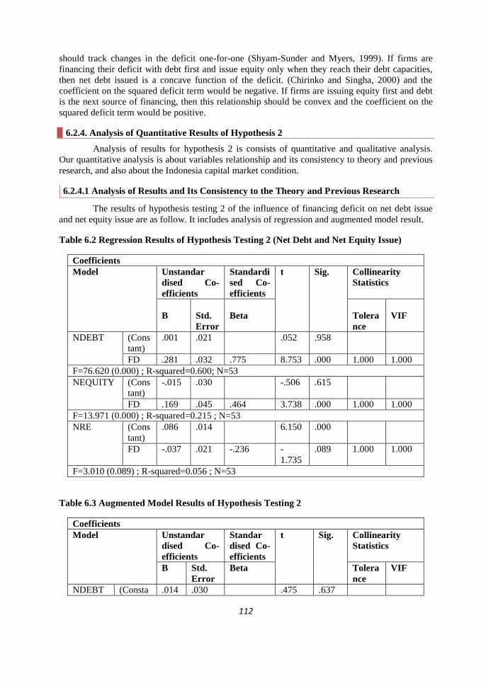
112
should track changes in the deficit one-for-one (Shyam-Sunder and Myers, 1999). If firms are
financing their deficit with debt first and issue equity only when they reach their debt capacities,
then net debt issued is a concave function of the deficit. (Chirinko and Singha, 2000) and the
coefficient on the squared deficit term would be negative. If firms are issuing equity first and debt
is the next source of financing, then this relationship should be convex and the coefficient on the
squared deficit term would be positive.
6.2.4. Analysis of Quantitative Results of Hypothesis 2
Analysis of results for hypothesis 2 is consists of quantitative and qualitative analysis.
Our quantitative analysis is about variables relationship and its consistency to theory and previous
research, and also about the Indonesia capital market condition.
6.2.4.1 Analysis of Results and Its Consistency to the Theory and Previous Research
The results of hypothesis testing 2 of the influence of financing deficit on net debt issue
and net equity issue are as follow. It includes analysis of regression and augmented model result.
Table 6.2 Regression Results of Hypothesis Testing 2 (Net Debt and Net Equity Issue)
Coefficients
Model Unstandar
dised Co-
efficients
Standardi
sed Co-
efficients
t Sig. Collinearity
Statistics
B
Std.
Error
Beta
Tolera
nce
VIF
NDEBT (Cons
tant)
.001 .021 .052 .958
FD .281 .032 .775 8.753 .000 1.000 1.000
F=76.620 (0.000) ; R-squared=0.600; N=53
NEQUITY (Cons
tant)
-.015 .030 -.506 .615
FD .169 .045 .464 3.738 .000 1.000 1.000
F=13.971 (0.000) ; R-squared=0.215 ; N=53
NRE (Cons
tant)
.086 .014 6.150 .000
FD -.037 .021 -.236 -
1.735
.089 1.000 1.000
F=3.010 (0.089) ; R-squared=0.056 ; N=53
Table 6.3 Augmented Model Results of Hypothesis Testing 2
Coefficients
Model Unstandar
dised Co-
efficients
Standar
dised Co-
efficients
t Sig. Collinearity
Statistics
B Std.
Error
Beta Tolera
nce
VIF
NDEBT (Consta .014 .030 .475 .637

113
nt)
FD .239 .075 .659 3.182 .003 .185 5.410
FDSQR .023 .037 .128 .618 .539 .185 5.410
Independent Variable: FD
F=38.037 (0.000) ; R-squared=0.603 ; Adjusted R-squared=0.588 ; N=53
A. Regression Model Result
Y is net debt issued and deficit is the financing deficit. This deficit is financed with debt
and/or equity. If firms follow the pecking order, changes in debt should track changes in the deficit
one-for-one. Therefore, the expected coefficient on the deficit is 1.
Net Debt Issued
From the tables we can conclude that the financing deficit has positive significant effects
on net debt issue with t-value of 8.753 and significance value of 0.000. This result suggests that
high deficit firms would tend to issue more net debt. However, the coefficient on the deficit is
0.281 and constant value is 0.001.
Net Equity Issued
The financing deficit has positive significant effects on net equity issue with t-value of
3.738 and significance value of 0.000. This result suggests that high deficit firms would tend to
issue more net equity. The coefficient on the deficit is 0.169 and constant value is -0.015.
Newly Retained Earning
The financing deficit has negative but not significant effects on newly retained earning with t-
value of -1.735 and significance value of 0.089. This result suggests that high deficit firms would
not tend to use newly retained earning. The coefficient on the deficit is -0.037 and constant value
is 0.086.
B. Augmented Model Result
The augmented model is an alternative means of accounting for a firm‟s debt capacity. If
firms are issuing equity first and debt is the next source of financing, then this relationship should
be convex and the coefficient on the squared deficit term would be positive.
For the augmented model, our result shows a positive coefficient on the financial deficit
and on the squared deficit term. However, for the squared deficit term, the coefficient was not
significant. A squared deficit coefficient that is not large in absolute value implies a less reliance
on equity finance for values of the financing deficit.
Table 6.4. Regression Results of Hypothesis Testing 2 (Issue Debt to Repurchase Equity)
Coefficients
Model Unstandar
dised Co-ef
ficients
Standardi
sed Co-
efficients
t Sig. Collinearity
Statistics
B Std.
Error
Beta Tolera
nce
VIF

114
Issue
Debt
(Constant) .025 .051 .502 .620
FD .179 .062 .508 2.890 .008 1.000 1.00
0
F=8.354 (0.008) ; R-squared=0.258 ; N=26
Repo
Equity
(Constant)
-.021
.020
-
1.054
.302
FD .000 .024 -.002 -.009 .993 1.000 1.00
0
Independent Variable: FD
F=0.000 (0.993) ; R-squared=3.18E-6 ; N=26
Issue Debt
From the tables we can conclude that the financing deficit has positive significant effects
on the net debt issue with t-value of 2.890 and significance value of 0.008. This result suggests
that high deficit firms would tend to issue more net debt. However, the coefficient on the deficit is
0.179 and constant value is 0.025.
Repurchase Equity
The financing deficit has negative but not significant effects on repurchase equity with t-
value of -0.009 and significance value of 0.993. This result suggests that high deficit firms would
not tend to repurchase equity. The coefficient on the deficit is 0.000 and constant value is -0.021.
From table 6.2-6.4, we concluded about firms preferring external or internal financing
and prefer debt or equity.
Prefer External or Internal Financing?
The coefficient of financing deficit on newly retained earning of the firms in the sample
is insignificantly negative. The coefficient of financing deficit on net debt and on net equity issue
is significantly positive. The coefficient of financing deficit on repurchase equity is insignificantly
negative. Therefore, we can conclude that our firms of sample prefer external to internal financing.
In addition, the firms would not repurchase equity to finance the deficit.
Prefer Debt or Equity?
The results of the firms that adopted the pecking order were consistent. The coefficient on
the deficit is significantly positive but the coefficient on the deficit-squared is insignificantly
positive. It indicates that firms issue debt at the first place, and debt is also the residual source of
financing once they have reached their debt capacities. Our evidence seems to suggest firms to rely
more heavily on debt financing rather than equity financing and it follows the pecking order
theory.
The pecking order theory states that changes in debt have played an important role in
assessing the pecking order theory. This is because the financing deficit is supposed to drive debt
according to this theory. Shyam-Sunder and Myers (1999) examined how debt responded to short-
term variation in investment and earnings. The theory predicts that when investments exceed
earnings, debt grows, and when earnings exceed investments, debt falls. Tests of the pecking order
115
theory define financing deficit as investments plus change in working capital plus dividends less
internal cash flow. The theory predicts that in a regression of net debt issues on the financing
deficit, the estimated slope coefficient should be one. The slope coefficient indicates the extent to
which new debt issues are explained by financing deficits.
Meanwhile, according to Myers (1984) a firm is said to follow a pecking order if it
prefers internal to external financing and debt to equity if external financing is used. In the Frank
and Goyal (2008) study, the definition of “prefer” internal financing can be interpreted in two
different views. The meaning could be that the firm uses all existing sources of internal finance
before issuing any debt or equity or “other things equal”, that the firm mostly uses internal
financing before using external financing. Meanwhile, they imply the strict interpretation of
“preference of debt over equity” which suggested that after the IPO, equity should never be issued
unless debt had for some reason become insufficient. This leads to the view of a “debt capacity”
which serves to limit the amount of debt and to allow for the use of equity within the pecking
order.
Pecking order models can be derived based on adverse selection considerations, agency
considerations, or other factors. There seem to be a couple of common features that inspire
pecking order theories. The first element is the linearity of the firm‟s objective function, which
means that costs tend to drive the results to corner solutions. The second common element of
pecking order models is the relative simplicity of the model (Frank and Goyal, 2008).
If we compared the previous research to our result, there were some research findings that
were not consistent with our results, for instance, previous research finding from Indonesia, (Ari
Christianti, 2008), concluded that: (1) The results of this study did not fully support the pecking
order theory in explaining the behaviour of firm financing in the IDX especially the manufacturing
sector. This could be explained from the results of the estimation that showed a negative and
significant coefficient of pecking order. (2) It might be explained from the results of this study that
the Indonesian capital market conditions were different from capital markets in developed
countries studied by Shyam-Sunder and Myers (1999), Frank and Goyal (2003) and Jong,
Verbeek, and Verwijmeren (2005). In addition, the impact of the economic crisis in 1997 still
affected the economic condition of Indonesia until 2005.
Leary and Roberts (2005) empirically examined the pecking order theory of capital
structure using a new empirical model that was motivated by the pecking order's decision rule and
implied financing hierarchy. They found that 62% (29%) of the firms in the sample were following
the pecking order in their decision between internal and external (debt and equity) financing and
that most of the equity issuing violations were not due to debt capacity concerns, as suggested by
the modified version of the pecking order. They showed empirically that the pecking order did not
seem to be an implication of information asymmetry.
The Cotei and Farhat (2008) study concluded that for the pecking order model, the test
results rejected the symmetric behaviour assumption at the industry level as well as across all
industries. Under the pecking order model, firms in financing deficit used debt to finance their new
investment whereas firms in financing surplus ended up retiring debt rather than repurchasing
equity. The results showed that firms had the tendency to reduce debt by a significantly higher
proportion when they had financing surplus compared to the proportion of debt issued when they
had financing deficit.
However, there were some research findings which were consistent to our results, for
example Sogorb-Mira and López-Gracia (2003) who explored pecking order theory and trade-off
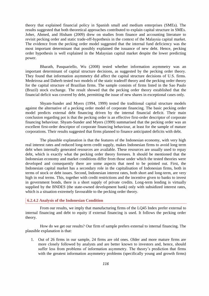
116
theory that explained financial policy in Spanish small and medium enterprises (SMEs). The
results suggested that both theoretical approaches contributed to explain capital structure in SMEs.
Joher, Ahmed, and Hisham (2009) drew on studies from finance and accounting literature to
revisit pecking order and static trade-off-hypothesis in the context of the Malaysia capital market.
The evidence from the pecking order model suggested that the internal fund deficiency was the
most important determinant that possibly explained the issuance of new debt. Hence, pecking
order hypothesis is well explained in the Malaysian capital market despite the lower predicting
power.
Bharath, Pasquariello, Wu (2008) tested whether information asymmetry was an
important determinant of capital structure decisions, as suggested by the pecking order theory.
They found that information asymmetry did affect the capital structure decisions of U.S. firms.
Medeirosa and Daherb tested two models of the static tradeoff theory and the pecking order theory
for the capital structure of Brazilian firms. The sample consists of firms listed in the Sao Paulo
(Brazil) stock exchange. The result showed that the pecking order theory established that the
financial deficit was covered by debt, permitting the issue of new shares in exceptional cases only.
Shyam-Sunder and Myers (1994, 1999) tested the traditional capital structure models
against the alternative of a pecking order model of corporate financing. The basic pecking order
model predicts external debt financing driven by the internal financial deficit. Their main
conclusion regarding pot is that the pecking order is an effective first-order descriptor of corporate
financing behaviour. Shyam-Sunder and Myers (1999) summarised that the pecking order was an
excellent first-order descriptor of corporate financing behaviour, at least for the sample of mature
corporations. Their results suggested that firms planned to finance anticipated deficits with debt.
The plausible explanation is that the features of the Indonesian economy, with very high
real interest rates and reduced long-term credit supply, makes Indonesian firms to avoid long term
debt when internally generated resources are available. These resources are usually used to repay
debt, which is exactly what the pecking order theory foresees. It should be mentioned that the
Indonesian economy and market conditions differ from those under which the tested theories were
developed and consequently there are some aspects that need to be pointed out. First, the
Indonesian capital market has a secondary role in the capitalisation of Indonesian firms, both in
terms of stock or debt issues. Second, Indonesian interest rates, both short and long-term, are very
high in real terms. This, together with credit restrictions and the incentive given to banks to invest
in government bonds, there is a short supply of private credits. Long-term lending is virtually
supplied by the BNDES (the state-owned development bank) only with subsidized interest rates,
which is a situation extremely favourable to the pecking order theory.
6.2.4.2 Analysis of the Indonesian Condition
From our results, we imply that manufacturing firms of the LQ45 Index prefer external to
internal financing and debt to equity if external financing is used. It follows the pecking order
theory.
How do we get our results? Our firm of sample prefers external to internal financing. The
plausible explanation is that:
1. Out of 26 firms in our sample, 24 firms are old ones. Older and more mature firms are
more closely followed by analysts and are better known to investors and, hence, should
suffer less from problems of information asymmetry. The theory‟s prediction that firms
with the greatest information asymmetry problems (specifically young and growth firms)

117
are precisely those that should be making financing choices according to the pecking
order.
However, in Indonesia all listed firms, including older-mature-large and young-growth-
small firms have less problems of information asymmetry as the government of Indonesia
has issued the regulations in order to make all listed firms announcing all information
about firms.
2. Firms in the manufacturing sector of the LQ45 Index firms have a good reputation to
mitigate the adverse selection problem between borrowers and lenders. In Indonesia, by
listing on the Indonesia Stock Exchange, banks will be more recognised and trusted than
companies. It is not excessive considering each moment banks can determine the condition
of the company's financials through various disclosure of information announced by the
company in the stock exchange. Rate of interest charged may also be lower considering
that the credit risk of public companies is relatively smaller.
3. Furthermore, older firms, more stable and highly profitable firms with few growth
opportunities and good credit histories are more suited to use external fund, both debt and
equity. Firms also have easier access to the company to enter into money markets through
the issuance of debt, both short and long term. Generally, the buyer of a letter of debt
would certainly prefer if the company issuing letters of debt has become a public company,
especially firms from the LQ45 Index.
4. However, some empirical evidence for the pecking order theory is inconsistent from our
results. The plausible explanation is that the Indonesian economy and market conditions
differ from those under which the previous research was developed.
If firms managers of manufacturing sector of the LQ45 issue equity, the most common
motivation based on the pecking order could be adverse selection developed by Myers and Majluf
(1984) and Myers (1984). The key idea is that the owner-manager of the firm knows the true value
of the firm‟s assets and growth opportunities. Outside investors can only guess these values. If the
manager offers to sell equity, then the outside investor must ask why the manager is willing to do
so. In many cases the manager of an overvalued firm will be happy to sell equity, while the
manager of an undervalued firm will not.
In the Indonesian capital market, by issuing equity, many benefits can be obtained by the
company including: obtaining large amounts of funds with costs of fund that are relatively smaller
than the funds obtained through banks, the various constraints and problems faced by the company
to survive and to develop are becoming the problems of stock holders by participating to think of
the best solutions so that the company can continue to grow, any increase in operational
performance and financial performance would have an impact on stock prices, which will
ultimately increase the value of the company.
6.2.5 Qualitative Analysis of Hypothesis 2
The following tables 6.5, 6.6a, 6.6b, 6.6c, 6.6d, are our research sample that consists of
26 firms and its classification, namely: growth (16 firms) and mature (10 firms), small (7 firms)
and large (19 firms), young (2 firms, INAF and KAEF) and old firms (24 firms).
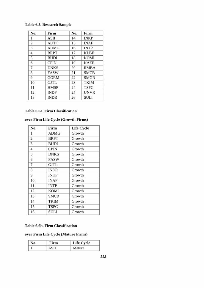
118
Table 6.5. Research Sample
No. Firm No. Firm
1 ASII 14 INKP
2 AUTO 15 INAF
3 ADMG 16 INTP
4 BRPT 17 KLBF
5 BUDI 18 KOMI
6 CPIN 19 KAEF
7 DNKS 20 RMBA
8 FASW 21 SMCB
9 GGRM 22 SMGR
10 GJTL 23 TKIM
11 HMSP 24 TSPC
12 INDF 25 UNVR
13 INDR 26 SULI
Table 6.6a. Firm Classification
over Firm Life Cycle (Growth Firms)
No. Firm Life Cycle
1 ADMG Growth
2 BRPT Growth
3 BUDI Growth
4 CPIN Growth
5 DNKS Growth
6 FASW Growth
7 GJTL Growth
8 INDR Growth
9 INKP Growth
10 INAF Growth
11 INTP Growth
12 KOMI Growth
13 SMCB Growth
14 TKIM Growth
15 TSPC Growth
16 SULI Growth
Table 6.6b. Firm Classification
over Firm Life Cycle (Mature Firms)
No. Firm Life Cycle
1 ASII Mature
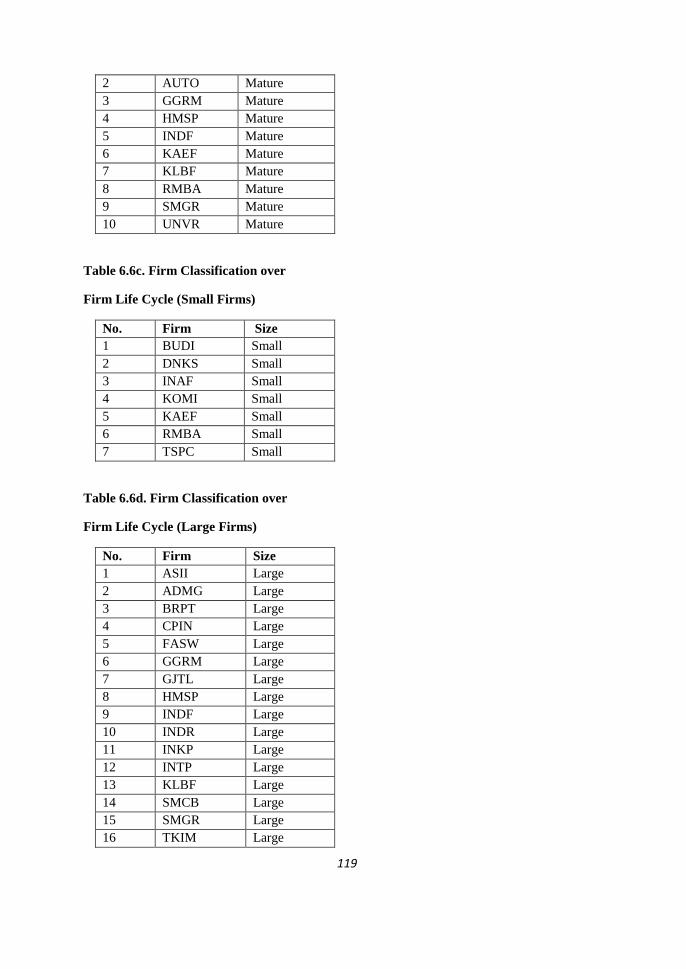
119
2 AUTO Mature
3 GGRM Mature
4 HMSP Mature
5 INDF Mature
6 KAEF Mature
7 KLBF Mature
8 RMBA Mature
9 SMGR Mature
10 UNVR Mature
Table 6.6c. Firm Classification over
Firm Life Cycle (Small Firms)
No. Firm Size
1 BUDI Small
2 DNKS Small
3 INAF Small
4 KOMI Small
5 KAEF Small
6 RMBA Small
7 TSPC Small
Table 6.6d. Firm Classification over
Firm Life Cycle (Large Firms)
No. Firm Size
1 ASII Large
2 ADMG Large
3 BRPT Large
4 CPIN Large
5 FASW Large
6 GGRM Large
7 GJTL Large
8 HMSP Large
9 INDF Large
10 INDR Large
11 INKP Large
12 INTP Large
13 KLBF Large
14 SMCB Large
15 SMGR Large
16 TKIM Large
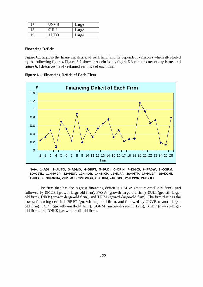
120
17 UNVR Large
18 SULI Large
19 AUTO Large
Financing Deficit
Figure 6.1 implies the financing deficit of each firm, and its dependent variables which illustrated
by the following figures. Figure 6.2 shows net debt issue, figure 6.3 explains net equity issue, and
figure 6.4 describes newly retained earnings of each firm.
Figure 6.1. Financing Deficit of Each Firm
The firm that has the highest financing deficit is RMBA (mature-small-old firm), and
followed by SMCB (growth-large-old firm), FASW (growth-large-old firm), SULI (growth-large-
old firm), INKP (growth-large-old firm), and TKIM (growth-large-old firm). The firm that has the
lowest financing deficit is BRPT (growth-large-old firm), and followed by UNVR (mature-large-
old firm), TSPC (growth-small-old firm), GGRM (mature-large-old firm), KLBF (mature-large-
old firm), and DNKS (growth-small-old firm).
Financing Deficit of Each Firm
0
0.2
0.4
0.6
0.8
1
1.2
1.4
1 2 3 4 5 6 7 8 9 10 11 12 13 14 15 16 17 18 19 20 21 22 23 24 25 26
firm
%
Note: 1=ASII, 2=AUTO, 3=ADMG, 4=BRPT, 5=BUDI, 6=CPIN, 7=DNKS, 8=FASW, 9=GGRM,
10=GJTL, 11=HMSP, 12=INDF, 13=INDR, 14=INKP, 15=INAF, 16=INTP, 17=KLBF, 18=KOMI,
19=KAEF, 20=RMBA, 21=SMCB, 22=SMGR, 23=TKIM, 24=TSPC, 25=UNVR, 26=SULI
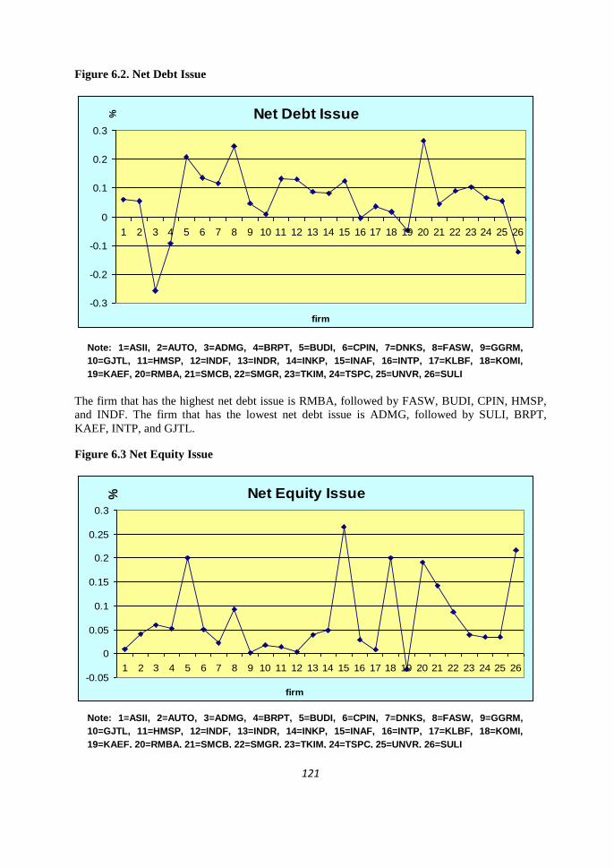
121
Figure 6.2. Net Debt Issue
The firm that has the highest net debt issue is RMBA, followed by FASW, BUDI, CPIN, HMSP,
and INDF. The firm that has the lowest net debt issue is ADMG, followed by SULI, BRPT,
KAEF, INTP, and GJTL.
Figure 6.3 Net Equity Issue
Net Debt Issue
-0.3
-0.2
-0.1
0
0.1
0.2
0.3
1 2 3 4 5 6 7 8 9 10 11 12 13 14 15 16 17 18 19 20 21 22 23 24 25 26
firm
%
Net Equity Issue
-0.05
0
0.05
0.1
0.15
0.2
0.25
0.3
1 2 3 4 5 6 7 8 9 10 11 12 13 14 15 16 17 18 19 20 21 22 23 24 25 26
firm
%
Note: 1=ASII, 2=AUTO, 3=ADMG, 4=BRPT, 5=BUDI, 6=CPIN, 7=DNKS, 8=FASW, 9=GGRM,
10=GJTL, 11=HMSP, 12=INDF, 13=INDR, 14=INKP, 15=INAF, 16=INTP, 17=KLBF, 18=KOMI,
19=KAEF, 20=RMBA, 21=SMCB, 22=SMGR, 23=TKIM, 24=TSPC, 25=UNVR, 26=SULI
Note: 1=ASII, 2=AUTO, 3=ADMG, 4=BRPT, 5=BUDI, 6=CPIN, 7=DNKS, 8=FASW, 9=GGRM,
10=GJTL, 11=HMSP, 12=INDF, 13=INDR, 14=INKP, 15=INAF, 16=INTP, 17=KLBF, 18=KOMI,
19=KAEF, 20=RMBA, 21=SMCB, 22=SMGR, 23=TKIM, 24=TSPC, 25=UNVR, 26=SULI
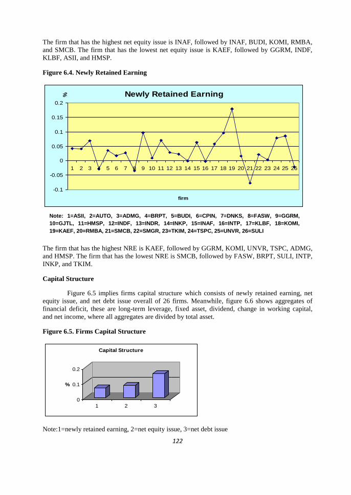
122
The firm that has the highest net equity issue is INAF, followed by INAF, BUDI, KOMI, RMBA,
and SMCB. The firm that has the lowest net equity issue is KAEF, followed by GGRM, INDF,
KLBF, ASII, and HMSP.
Figure 6.4. Newly Retained Earning
The firm that has the highest NRE is KAEF, followed by GGRM, KOMI, UNVR, TSPC, ADMG,
and HMSP. The firm that has the lowest NRE is SMCB, followed by FASW, BRPT, SULI, INTP,
INKP, and TKIM.
Capital Structure
Figure 6.5 implies firms capital structure which consists of newly retained earning, net
equity issue, and net debt issue overall of 26 firms. Meanwhile, figure 6.6 shows aggregates of
financial deficit, these are long-term leverage, fixed asset, dividend, change in working capital,
and net income, where all aggregates are divided by total asset.
Figure 6.5. Firms Capital Structure
Note:1=newly retained earning, 2=net equity issue, 3=net debt issue
Newly Retained Earning
-0.1
-0.05
0
0.05
0.1
0.15
0.2
1 2 3 4 5 6 7 8 9 10 11 12 13 14 15 16 17 18 19 20 21 22 23 24 25 26
firm
%
0
0.1
0.2
%
1 2 3
Capital Structure
Note: 1=ASII, 2=AUTO, 3=ADMG, 4=BRPT, 5=BUDI, 6=CPIN, 7=DNKS, 8=FASW, 9=GGRM,
10=GJTL, 11=HMSP, 12=INDF, 13=INDR, 14=INKP, 15=INAF, 16=INTP, 17=KLBF, 18=KOMI,
19=KAEF, 20=RMBA, 21=SMCB, 22=SMGR, 23=TKIM, 24=TSPC, 25=UNVR, 26=SULI
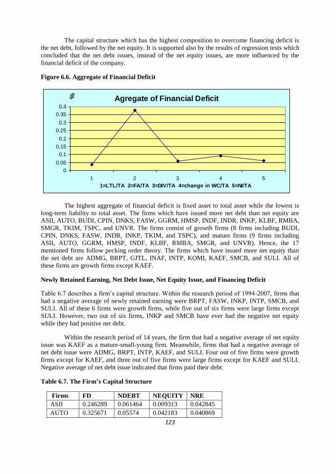
123
The capital structure which has the highest composition to overcome financing deficit is
the net debt, followed by the net equity. It is supported also by the results of regression tests which
concluded that the net debt issues, instead of the net equity issues, are more influenced by the
financial deficit of the company.
Figure 6.6. Aggregate of Financial Deficit
The highest aggregate of financial deficit is fixed asset to total asset while the lowest is
long-term liability to total asset. The firms which have issued more net debt than net equity are
ASII, AUTO, BUDI, CPIN, DNKS, FASW, GGRM, HMSP, INDF, INDR, INKP, KLBF, RMBA,
SMGR, TKIM, TSPC, and UNVR. The firms consist of growth firms (8 firms including BUDI,
CPIN, DNKS, FASW, INDR, INKP, TKIM, and TSPC), and mature firms (9 firms including
ASII, AUTO, GGRM, HMSP, INDF, KLBF, RMBA, SMGR, and UNVR). Hence, the 17
mentioned firms follow pecking order theory. The firms which have issued more net equity than
the net debt are ADMG, BRPT, GJTL, INAF, INTP, KOMI, KAEF, SMCB, and SULI. All of
these firms are growth firms except KAEF.
Newly Retained Earning, Net Debt Issue, Net Equity Issue, and Financing Deficit
Table 6.7 describes a firm‟s capital structure. Within the research period of 1994-2007, firms that
had a negative average of newly retained earning were BRPT, FASW, INKP, INTP, SMCB, and
SULI. All of these 6 firms were growth firms, while five out of six firms were large firms except
SULI. However, two out of six firms, INKP and SMCB have ever had the negative net equity
while they had positive net debt.
Within the research period of 14 years, the firm that had a negative average of net equity
issue was KAEF as a mature-small-young firm. Meanwhile, firms that had a negative average of
net debt issue were ADMG, BRPT, INTP, KAEF, and SULI. Four out of five firms were growth
firms except for KAEF, and three out of five firms were large firms except for KAEF and SULI.
Negative average of net debt issue indicated that firms paid their debt.
Table 6.7. The Firm’s Capital Structure
Firms FD NDEBT NEQUITY NRE
ASII 0.246289 0.061464 0.009313 0.042845
AUTO 0.325671 0.05574 0.042183 0.040869
Agregate of Financial Deficit
0
0.05
0.1
0.15
0.2
0.25
0.3
0.35
0.4
1 2 3 4 5
1=LTL/TA 2=FA/TA 3=DIV/TA 4=change in WC/TA 5=NI/TA
%
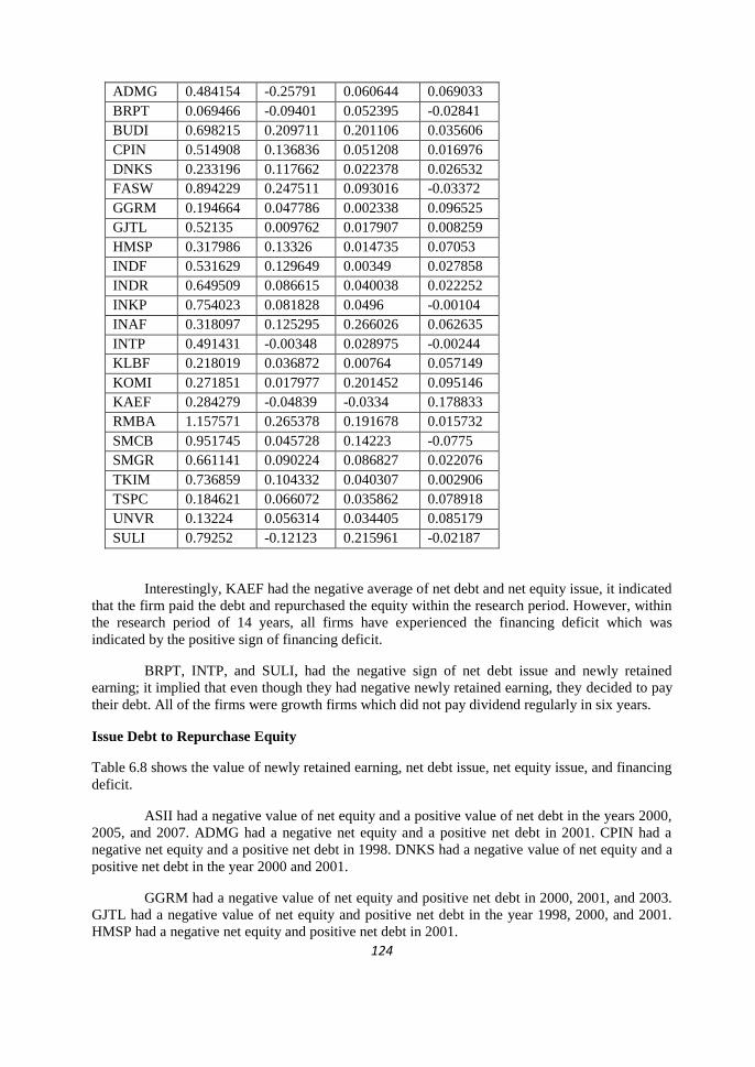
124
ADMG 0.484154 -0.25791 0.060644 0.069033
BRPT 0.069466 -0.09401 0.052395 -0.02841
BUDI 0.698215 0.209711 0.201106 0.035606
CPIN 0.514908 0.136836 0.051208 0.016976
DNKS 0.233196 0.117662 0.022378 0.026532
FASW 0.894229 0.247511 0.093016 -0.03372
GGRM 0.194664 0.047786 0.002338 0.096525
GJTL 0.52135 0.009762 0.017907 0.008259
HMSP 0.317986 0.13326 0.014735 0.07053
INDF 0.531629 0.129649 0.00349 0.027858
INDR 0.649509 0.086615 0.040038 0.022252
INKP 0.754023 0.081828 0.0496 -0.00104
INAF 0.318097 0.125295 0.266026 0.062635
INTP 0.491431 -0.00348 0.028975 -0.00244
KLBF 0.218019 0.036872 0.00764 0.057149
KOMI 0.271851 0.017977 0.201452 0.095146
KAEF 0.284279 -0.04839 -0.0334 0.178833
RMBA 1.157571 0.265378 0.191678 0.015732
SMCB 0.951745 0.045728 0.14223 -0.0775
SMGR 0.661141 0.090224 0.086827 0.022076
TKIM 0.736859 0.104332 0.040307 0.002906
TSPC 0.184621 0.066072 0.035862 0.078918
UNVR 0.13224 0.056314 0.034405 0.085179
SULI 0.79252 -0.12123 0.215961 -0.02187
Interestingly, KAEF had the negative average of net debt and net equity issue, it indicated
that the firm paid the debt and repurchased the equity within the research period. However, within
the research period of 14 years, all firms have experienced the financing deficit which was
indicated by the positive sign of financing deficit.
BRPT, INTP, and SULI, had the negative sign of net debt issue and newly retained
earning; it implied that even though they had negative newly retained earning, they decided to pay
their debt. All of the firms were growth firms which did not pay dividend regularly in six years.
Issue Debt to Repurchase Equity
Table 6.8 shows the value of newly retained earning, net debt issue, net equity issue, and financing
deficit.
ASII had a negative value of net equity and a positive value of net debt in the years 2000,
2005, and 2007. ADMG had a negative net equity and a positive net debt in 2001. CPIN had a
negative net equity and a positive net debt in 1998. DNKS had a negative value of net equity and a
positive net debt in the year 2000 and 2001.
GGRM had a negative value of net equity and positive net debt in 2000, 2001, and 2003.
GJTL had a negative value of net equity and positive net debt in the year 1998, 2000, and 2001.
HMSP had a negative net equity and positive net debt in 2001.
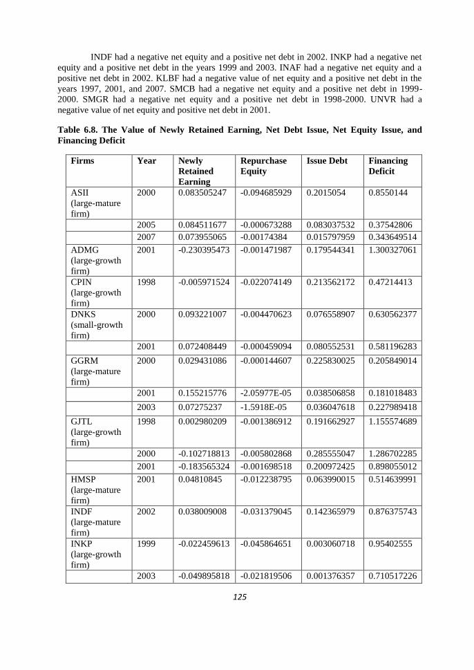
125
INDF had a negative net equity and a positive net debt in 2002. INKP had a negative net
equity and a positive net debt in the years 1999 and 2003. INAF had a negative net equity and a
positive net debt in 2002. KLBF had a negative value of net equity and a positive net debt in the
years 1997, 2001, and 2007. SMCB had a negative net equity and a positive net debt in 1999-
2000. SMGR had a negative net equity and a positive net debt in 1998-2000. UNVR had a
negative value of net equity and positive net debt in 2001.
Table 6.8. The Value of Newly Retained Earning, Net Debt Issue, Net Equity Issue, and
Financing Deficit
Firms Year Newly
Retained
Earning
Repurchase
Equity
Issue Debt Financing
Deficit
ASII
(large-mature
firm)
2000 0.083505247 -0.094685929 0.2015054 0.8550144
2005 0.084511677 -0.000673288 0.083037532 0.37542806
2007 0.073955065 -0.00174384 0.015797959 0.343649514
ADMG
(large-growth
firm)
2001 -0.230395473 -0.001471987 0.179544341 1.300327061
CPIN
(large-growth
firm)
1998 -0.005971524 -0.022074149 0.213562172 0.47214413
DNKS
(small-growth
firm)
2000 0.093221007 -0.004470623 0.076558907 0.630562377
2001 0.072408449 -0.000459094 0.080552531 0.581196283
GGRM
(large-mature
firm)
2000 0.029431086 -0.000144607 0.225830025 0.205849014
2001 0.155215776 -2.05977E-05 0.038506858 0.181018483
2003 0.07275237 -1.5918E-05 0.036047618 0.227989418
GJTL
(large-growth
firm)
1998 0.002980209 -0.001386912 0.191662927 1.155574689
2000 -0.102718813 -0.005802868 0.285555047 1.286702285
2001 -0.183565324 -0.001698518 0.200972425 0.898055012
HMSP
(large-mature
firm)
2001 0.04810845 -0.012238795 0.063990015 0.514639991
INDF
(large-mature
firm)
2002 0.038009008 -0.031379045 0.142365979 0.876375743
INKP
(large-growth
firm)
1999 -0.022459613 -0.045864651 0.003060718 0.95402555
2003 -0.049895818 -0.021819506 0.001376357 0.710517226
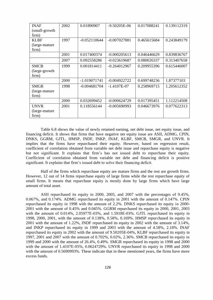
126
INAF
(small-growth
firm)
2002 0.01890907 -9.50205E-06 0.017088241 0.139112319
KLBF
(large-mature
firm)
1997 -0.052110644 -0.007027881 0.465615684 0.243849179
2001 0.017400374 -0.000205613 0.046446629 0.839836767
2007 0.092558286 -0.023619687 0.080026337 0.313407658
SMCB
(large-growth
firm)
1999 0.001814411 -0.264012967 0.209955396 0.615446007
2000 -1.019071741 -0.004922722 0.699748236 1.87377103
SMGR
(large-mature
firm)
1998 -0.004681704 -1.4107E-07 0.258969715 1.205612352
2000 0.032699452 -0.000624729 0.017395451 1.112214508
UNVR
(large-mature
firm)
2001 0.118556144 -0.005690993 0.046673976 0.077622313
Table 6.8 shows the value of newly retained earning, net debt issue, net equity issue, and
financing deficit. It shows that firms that have negative net equity issue are ASII, ADMG, CPIN,
DNKS, GGRM, GJTL, HMSP, INDF, INKP, INAF, KLBF, SMCB, SMGR, and UNVR. It
implies that the firms have repurchased their equity. However, based on regression result,
coefficient of correlation obtained from variable net debt issue and repurchase equity is negative
but not significant. It explains that firm‟s has not issued debt to repurchase their equity.
Coefficient of correlation obtained from variable net debt and financing deficit is positive
significant. It explains that firm‟s issued debt to solve their financing deficit.
Half of the firms which repurchase equity are mature firms and the rest are growth firms.
However, 12 out of 14 firms repurchase equity of large firms while the rest repurchase equity of
small firms. It means that repurchase equity is mostly done by large firms which have large
amount of total asset.
ASII repurchased its equity in 2000, 2005, and 2007 with the percentages of 9.45%,
0.067%, and 0.174%. ADMG repurchased its equity in 2001 with the amount of 0.147%. CPIN
repurchased its equity in 1998 with the amount of 2.2%. DNKS repurchased its equity in 2000-
2001 with the amount of 0.45% and 0.045%. GGRM repurchased its equity in 2000, 2001, 2003
with the amount of 0.014%, 2.05977E-03%, and 1.5918E-03%. GJTL repurchased its equity in
1998, 2000, 2001, with the amount of 0.138%, 0.58%, 0.169%. HMSP repurchased its equity in
2001 with the amount of 1.22%, INDF repurchased its equity in 2002 with the amount of 3.14%,
and INKP repurchased its equity in 1999 and 2003 with the amount of 4.58%, 2.18%. INAF
repurchased its equity in 2002 with the amount of 9.50205E-04%, KLBF repurchased its equity in
1997, 2001 and 2007 with the amount of 0.702%, 0.02%, 2.36%. SMCB repurchased its equity in
1999 and 2000 with the amount of 26.4%, 0.49%. SMGR repurchased its equity in 1998 and 2000
with the amount of 1.4107E-05%, 0.0624729%. UNVR repurchased its equity in 1998 and 2000
with the amount of 0.5690993%. These indicate that in these mentioned years, the firms have more
excess funds.
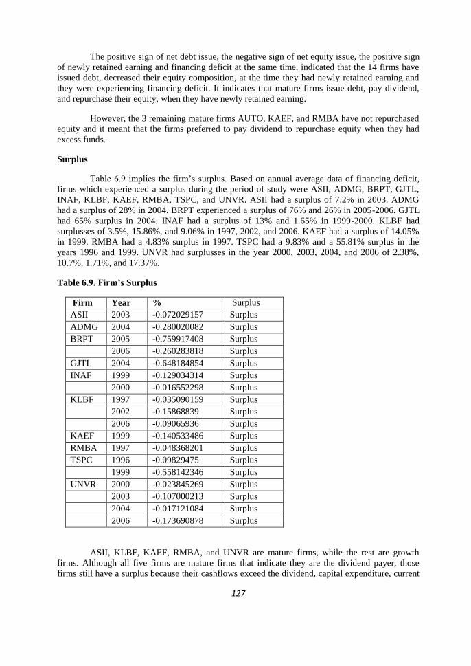
127
The positive sign of net debt issue, the negative sign of net equity issue, the positive sign
of newly retained earning and financing deficit at the same time, indicated that the 14 firms have
issued debt, decreased their equity composition, at the time they had newly retained earning and
they were experiencing financing deficit. It indicates that mature firms issue debt, pay dividend,
and repurchase their equity, when they have newly retained earning.
However, the 3 remaining mature firms AUTO, KAEF, and RMBA have not repurchased
equity and it meant that the firms preferred to pay dividend to repurchase equity when they had
excess funds.
Surplus
Table 6.9 implies the firm‟s surplus. Based on annual average data of financing deficit,
firms which experienced a surplus during the period of study were ASII, ADMG, BRPT, GJTL,
INAF, KLBF, KAEF, RMBA, TSPC, and UNVR. ASII had a surplus of 7.2% in 2003. ADMG
had a surplus of 28% in 2004. BRPT experienced a surplus of 76% and 26% in 2005-2006. GJTL
had 65% surplus in 2004. INAF had a surplus of 13% and 1.65% in 1999-2000. KLBF had
surplusses of 3.5%, 15.86%, and 9.06% in 1997, 2002, and 2006. KAEF had a surplus of 14.05%
in 1999. RMBA had a 4.83% surplus in 1997. TSPC had a 9.83% and a 55.81% surplus in the
years 1996 and 1999. UNVR had surplusses in the year 2000, 2003, 2004, and 2006 of 2.38%,
10.7%, 1.71%, and 17.37%.
Table 6.9. Firm’s Surplus
Firm Year % Surplus
ASII 2003 -0.072029157 Surplus
ADMG 2004 -0.280020082 Surplus
BRPT 2005 -0.759917408 Surplus
2006 -0.260283818 Surplus
GJTL 2004 -0.648184854 Surplus
INAF 1999 -0.129034314 Surplus
2000 -0.016552298 Surplus
KLBF 1997 -0.035090159 Surplus
2002 -0.15868839 Surplus
2006 -0.09065936 Surplus
KAEF 1999 -0.140533486 Surplus
RMBA 1997 -0.048368201 Surplus
TSPC 1996 -0.09829475 Surplus
1999 -0.558142346 Surplus
UNVR 2000 -0.023845269 Surplus
2003 -0.107000213 Surplus
2004 -0.017121084 Surplus
2006 -0.173690878 Surplus
ASII, KLBF, KAEF, RMBA, and UNVR are mature firms, while the rest are growth
firms. Although all five firms are mature firms that indicate they are the dividend payer, those
firms still have a surplus because their cashflows exceed the dividend, capital expenditure, current
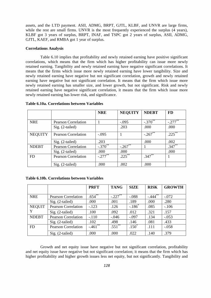
128
assets, and the LTD payment. ASII, ADMG, BRPT, GJTL, KLBF, and UNVR are large firms,
while the rest are small firms. UNVR is the most frequently experienced the surplus (4 years),
KLBF got 3 years of surplus, BRPT, INAF, and TSPC got 2 years of surplus, ASII, ADMG,
GJTL, KAEF, and RMBA got 1 year of surplus.
Correlations Analysis
Table 6.10 implies that profitability and newly retained earning have positive significant
correlations, which means that the firm which has higher profitability can issue more newly
retained earning. Tangibility and newly retained earning have negative significant correlations. It
means that the firms which issue more newly retained earning have lower tangibility. Size and
newly retained earning have negative but not significant correlation, growth and newly retained
earning have negative but not significant correlation. It means that the firm which issue more
newly retained earning has smaller size, and lower growth, but not significant. Risk and newly
retained earning have negative significant correlation, it means that the firm which issue more
newly retained earning has lower risk, and significance.
Table 6.10a. Correlations between Variables
NRE NEQUITY NDEBT FD
NRE Pearson Correlation 1 -.095 -.370**
-.277**
Sig. (2-tailed) .203 .000 .000
NEQUITY Pearson Correlation -.095 1 -.267**
.225**
Sig. (2-tailed) .203 .000 .002
NDEBT Pearson Correlation -.370**
-.267**
1 .347**
Sig. (2-tailed) .000 .000 .000
FD Pearson Correlation -.277**
.225**
.347**
1
Sig. (2-tailed) .000 .002 .000
Table 6.10b. Correlations between Variables
PRFT TANG SIZE RISK GROWTH
NRE Pearson Correlation .654**
-.227**
-.088 -.444**
-.072
Sig. (2-tailed) .000 .001 .189 .000 .280
NEQUIT
Y
Pearson Correlation -.123 .126 -.186* .085 -.106
Sig. (2-tailed) .100 .092 .012 .321 .157
NDEBT Pearson Correlation -.110 -.046 -.097 .134 -.053
Sig. (2-tailed) .102 .498 .146 .081 .433
FD Pearson Correlation -.461**
.551**
.150* .111 -.058
Sig. (2-tailed) .000 .000 .022 .140 .379
Growth and net equity issue have negative but not significant correlation, profitability
and net equity issue have negative but not significant correlation; it means that the firm which has
higher profitability and higher growth issues less net equity, but not significantly. Tangibility and

129
net equity issue have positive but not significant correlation, risk and net equity issue have positive
but not significant correlation, it means that the firm which has higher tangibility and higher risk
issues more net equity, but not significantly. Size and net equity issue have negative significant
correlation, it means that the firm which has larger size and issue less net equity, and significantly.
Profitability and net debt issue have negative but not significant correlation, tangibility
and net debt issue have negative but not significant correlation, size and net debt issue have
negative but not significant correlation, growth and net debt issue have negative but not significant
correlation; it means that the firm which has larger size, higher profitability, tangibility, and
growth, issues less net equity, but not significantly. Risk and net debt issue have positive but not
significant correlation. It means that the firm which has higher risk, issues more net debt, but not
significantly.
Profitability and financing deficit have negative significant correlation; it means that the
firm which has higher financing deficit has lower profitability, and the correlation is significant.
Growth and financing deficit have negative but not significant correlation; it means that the firm
which has higher financing deficit has lower growth, but it is not significant. Tangibility and
financing deficit have positive significant correlation, Size and financing deficit have positive
significant correlation, it means that the firm which has higher financing deficit, is a larger firm,
and has higher asset tangibility, and the correlation is significant. Risk and financing deficit have
positive but not significant correlation, it means that the firm which has higher financing deficit, is
high risk firm, but not significant.
6.3. Research Question 3, Hypothesis, Hypothesis Testing, and Result Analysis
As applied in hypothesis 1, we also use quantitative strategy in testing hypothesis 3. The following
sub-sections are explaining research questions three, hypotheses three, hypotheses testing three,
and results analysis.
6.3.1. Research Question Three
Based on the asymmetric information and signalling theory, our major and minor
research questions are as follow:
Does debt policy matter?
(a) If firms issue new debt, what will happen to the firm‟s stock price?
(b) If firms issue new equity, what will happen to the firm‟s stock price?
(c) If firms issue debt to repurchase equity, what will happen to the firm‟s stock price?
6.3.2. Hypothesis 3
By formulating research question three, therefore, our major and minor hypotheses three
are as follow:
Debt does policy matter.
(a) If firms issue new debt, then the firms‟s stock price will be higher.
(b) If firms issue new equity, then the firms‟s stock price will be lower.
(c) If firms issue debt to repurchase equity, then the firms‟s stock price will be higher.
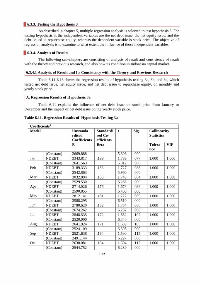
130
6.3.3. Testing the Hypothesis 3
As described in chapter 5, multiple regression analysis is selected to test hypothesis 3. For
testing hypothesis 3, the independent variables are the net debt issue, the net equity issue, and the
debt issued to repurchase equity, whereas the dependent variable is stock price. The objective of
regression analysis is to examine to what extent the influence of those independent variables.
6.3.4. Analysis of Results
The following sub-chapters are consisting of analysis of result and consistency of result
with the theory and previous research, and also how its condition in Indonesia capital market.
6.3.4.1 Analysis of Result and Its Consistency with the Theory and Previous Research
Table 6.11-6.13 shows the regression results of hypothesis testing 3a, 3b, and 3c, which
tested net debt issue, net equity issue, and net debt issue to repurchase equity, on monthly and
yearly stock price.
A. Regression Results of Hypothesis 3a
Table 6.11 explains the influence of net debt issue on stock price from January to
December and the impact of net debt issue on the yearly stock price.
Table 6.11. Regression Results of Hypothesis Testing 3a
Coefficientsa
Model Unstanda
rdised
Coefficients
Standardi
sed Co-
efficients
t Sig. Collinearity
Statistics
B Beta Tolera
nce
VIF
Jan
(Constant) 2669.888 5.806 .000
NDEBT 3343.817 .189 1.789 .077 1.000 1.000
Feb
(Constant) 2641.563 5.812 .000
NDEBT 3189.333 .183 1.727 .088 1.000 1.000
Mar
(Constant) 2542.863 5.960 .000
NDEBT 3032.894 .185 1.749 .084 1.000 1.000
Apr
(Constant) 2529.530 6.288 .000
NDEBT 2714.026 .176 1.673 .098 1.000 1.000
May
(Constant) 2590.855 6.400 .000
NDEBT 2812.141 .181 1.722 .089 1.000 1.000
Jun
(Constant) 2588.295 6.510 .000
NDEBT 2780.620 .182 1.734 .086 1.000 1.000
Jul
(Constant) 2674.262 6.287 .000
NDEBT 2848.535 .172 1.652 .102 1.000 1.000
Aug
(Constant) 2520.000 6.340 .000
NDEBT 2641.924 .171 1.639 .105 1.000 1.000
Sep
(Constant) 2524.109 6.508 .000
NDEBT 2521.638 .164 1.590 .115 1.000 1.000
Oct
(Constant) 2491.144 6.227 .000
NDEBT 2638.081 .164 1.604 .112 1.000 1.000
(Constant) 2544.752 6.289 .000
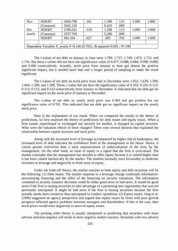
131
Nov NDEBT 2669.798 .161 1.589 .115 1.000 1.000
Dec
(Constant) 2642.126 6.410 .000
NDEBT 2786.625 .159 1.598 .113 1.000 1.000
yearly (Constant) 3557.769 5.286 .000
NDEBT 945.164 .027 .383 .702 1.000 1.000
Dependent Variable: P_yearly F=0.146 (0.702) ; R-squared=0.001 ; N=196
The t-values of net debt on January to June were 1.789; 1.727; 1.749; 1.673; 1.722; and
1.734. But these t-values did not have the significance value of 0.077; 0.088; 0.084; 0.098; 0.089;
and 0.086 consecutively. Actually, stock price from January to June got almost the positive
significant impact, but it needed more data and a longer period of sampling to make the result
significant.
The t-values of net debt on stock price from July to December were 1.652; 1.639; 1.590;
1.604; 1.589; and 1.598. Those, t-value did not have the significance value of 0.102; 0.105; 0.115;
0.112; 0.115; and 0.133 consecutively from January to December. It indicated that net debt got no
significant impact on the stock price of January to December.
The t-value of net debt on yearly stock price was 0.383 and got positive but not
significance value of 0.702. This indicated that net debt got no significant impact on the yearly
stock price.
Here is the explanation of our result. When we compared the results to the theory of
predictions, we first analysed the theory of predictions for debt issues and equity issues. When a
firm issued, repurchased or exchanged one security for another, it changed its capital structure.
What were the valuation effects of these changes? There were several theories that explained the
relationship between capital structure and stock price.
Along with the increased level of leverage accompanied by higher risk of bankruptcy, the
increased level of debt indicates the confidence level of the management in the future. Hence, it
carries greater conviction than a mere announcement of undervaluation of the firm, by the
management. On the other hand, an issue of equity is a signal that the firm is overvalued. The
market concludes that the management has decided to offer equity because it is valued higher than
it has been valued intrinsically by the market. The markets normally react favourably to moderate
increases in leverage and negatively to fresh issue of equity.
Under the trade-off theory, the market reaction to both equity and debt securities will be
the following: (1) Debt issues. The market response to a leverage change confounds information:
necessitating financing and the effect of the financing on security valuations. The information
contained in security issuance decisions could be either good news or bad news. It would be good
news if the firm is issuing securities to take advantage of a promising new opportunity that was not
previously anticipated. It might be bad news if the firm is issuing securities because the firm
actually needs more resources than anticipated to conduct operations. (2) Equity issues. Jung et al.
(1996) suggested an agency perspective and argued that equity issues by firms with poor growth
prospects reflected agency problems between managers and shareholders. If this is the case, then
stock prices would react negatively to news of equity issues.
The pecking order theory is usually interpreted as predicting that securities with more
adverse selection (equity) will result in more negative market reaction. Securities with less adverse

132
selection (debt) will result in less negative or no market reaction. This of course, still rest on some
assumptions about market anticipations.
Conclusion: Our result is positive. Therefore, our result is consistent with signalling
through capital structure, as the increased level of leverage is accompanied by higher risk of
bankruptcy, the increased level of debt indicates the confidence of the management in the future.
Hence it carries greater conviction than a mere announcement of undervaluation of the firm by the
management.
Our result is also consistent with the pecking order theory, as securities with less adverse
selection (debt) will result in less negative or no market reaction. Finally, our result is in line with
trade off theory. If the firm issued securities to take advantage of a promising new opportunity, so
it would be good news to the market.
If compared to previous empirical evidence, our result is consistent with the following
findings, for example, announcements of ordinary debt issues generate zero market reaction on
average (Eckbo (1986) and Antweiler and Frank (2006)). The zero market reaction to corporate
debt issues is robust to various attempts to control for partial anticipation. Meanwhile, exchange of
common for debt/preferred stock generates positive stock price reactions while exchange of
debt/preferred for common stock generates negative reactions (Masulis, 1980a). Eckbo and
Masulis (1995) concluded that announcements of security issues typically generated a non-positive
stock price reaction.
Ross (1977) showed that good corporate performance could give a signal with a high
portion of debt in their capital structure. Ross (1977) assumed firms that were less well
performancing would not use debt in large portion as it would be followed by the high chance of
bankruptcy. By using these assumptions in which the company will use the good performance of
higher debt, while firms that are less good performance will use more of equity. Ross (1977)
assumed that investors would be able to distinguish the company's performance by looking at the
company's capital structure and they will give a higher value on the company with larger debt
portion. It indicates that the result do not support the stated of signalling theory. The result
indicates that the greater the leverage, the greater the possibility of financial distress leading to
bankruptcy. When the company went bankrupt, shareholders would lose money they invest in the
company (Peirson et al, 2002).
However, our result is inconsistent with the following empirical evidence. In Indonesia,
the regression coefficient between leverage and stock price is significantly negative. The use of
high leverage will be responded by the market with a fall in stock prices. These results are
consistent with the findings of a negative relationship between leverage and stock price as
proposed by Frank and Goyal (2003). Relationship between the two variables will be positive at
the time the company has many tangible assets that will secure leverage of companies.
Announcements of convertible debt issues resulted in mildly negative stock price
reactions (such as Dann and Mikkelson, 1984; Mikkelson and Partch, 1986). The valuation effects
are the most negative for common stock issues, slightly less negative for convertible debt issues
and least negative (zero) for straight debt issues. The effects are more negative the larger the issue.
The reason of why firms issue debt could be the intention to take advantage, eventhough
there would be the disadvantages of debt. Indonesia companies face the challenge of determining
whether to issue debt or equity for financing needs.
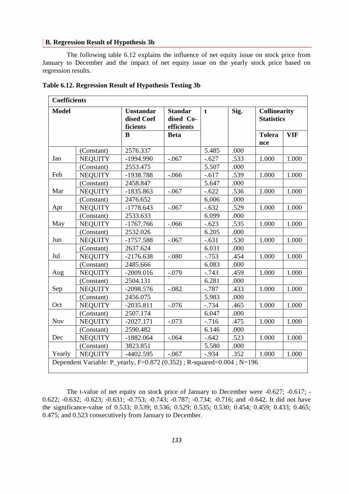
133
B. Regression Result of Hypothesis 3b
The following table 6.12 explains the influence of net equity issue on stock price from
January to December and the impact of net equity issue on the yearly stock price based on
regression results.
Table 6.12. Regression Result of Hypothesis Testing 3b
Coefficients
Model Unstandar
dised Coef
ficients
Standar
dised Co-
efficients
t Sig. Collinearity
Statistics
B Beta Tolera
nce
VIF
Jan
(Constant) 2576.337 5.485 .000
NEQUITY -1994.990 -.067 -.627 .533 1.000 1.000
Feb
(Constant) 2553.475 5.507 .000
NEQUITY -1938.788 -.066 -.617 .539 1.000 1.000
Mar
(Constant) 2458.847 5.647 .000
NEQUITY -1835.863 -.067 -.622 .536 1.000 1.000
Apr
(Constant) 2476.652 6.006 .000
NEQUITY -1778.643 -.067 -.632 .529 1.000 1.000
May
(Constant) 2533.633 6.099 .000
NEQUITY -1767.766 -.066 -.623 .535 1.000 1.000
Jun
(Constant) 2532.026 6.205 .000
NEQUITY -1757.588 -.067 -.631 .530 1.000 1.000
Jul
(Constant) 2637.624 6.031 .000
NEQUITY -2176.638 -.080 -.753 .454 1.000 1.000
Aug
(Constant) 2485.666 6.083 .000
NEQUITY -2009.016 -.079 -.743 .459 1.000 1.000
Sep
(Constant) 2504.131 6.281 .000
NEQUITY -2098.576 -.082 -.787 .433 1.000 1.000
Oct
(Constant) 2456.075 5.983 .000
NEQUITY -2035.811 -.076 -.734 .465 1.000 1.000
Nov
(Constant) 2507.174 6.047 .000
NEQUITY -2027.171 -.073 -.716 .475 1.000 1.000
Dec
(Constant) 2590.482 6.146 .000
NEQUITY -1882.064 -.064 -.642 .523 1.000 1.000
Yearly
(Constant) 3823.851 5.580 .000
NEQUITY -4402.595 -.067 -.934 .352 1.000 1.000
Dependent Variable: P_yearly, F=0.872 (0.352) ; R-squared=0.004 ; N=196
The t-value of net equity on stock price of January to December were -0.627; -0.617; -
0.622; -0.632; -0.623; -0.631; -0.753; -0.743; -0.787; -0.734; -0.716; and -0.642. It did not have
the significance-value of 0.533; 0.539; 0.536; 0.529; 0.535; 0.530; 0.454; 0.459; 0.433; 0.465;
0.475; and 0.523 consecutively from January to December.

134
The t-value of net equity on yearly stock price was -0.934 and got negative but not
significance value of 0.352. This indicated that net equity had no significant impact on the yearly
stock price. This result suggests that firms that issue more net equity would tend to have
decreasing stock price. Thus, we fail to reject the hypothesis that if firms issue new equity, then
the firm‟s stock price will be lower.
Here is the explanation of our result. When we compared the results to the theory of
predictions, our results were consistent with the theory of signalling through capital structure,
pecking order theory, and Jung et al. (1996). Jung et al. (1996) suggested an agency perspective
and argued that equity issues by firms with poor growth prospects reflected agency problems
between managers and shareholders. If this is the case, then stock prices would react negatively to
news of equity issues. Our results were consistent with the following empirical evidence, for
instance, announcements of equity issues resulted in significant negative stock price reactions
(Asquith and Mullins Jr., 1986; Masulis and Korwar, 1986; and Antweiler and Frank, 2006).
The negative market reaction to equity issues and zero market reaction to debt issues are
consistent with adverse selection arguments. Indeed, there is other interpretation. Jung et al. (1996)
showed that firms without valuable investment opportunities experienced a more negative stock
price reaction to equity issues than did firms with better investment opportunities. Thus, agency
cost arguments could also explain the existing evidence on security issues. Further support for the
agency view came from the finding that firms without valuable investment opportunities issuing
equity invested more than similar firms issuing debt and that firms with low managerial ownership
had worse stock price reaction to new equity issue announcements than did firms with high
managerial ownership.
Meanwhile, our results were inconsistent with the following empirical evidence. The
impact of equity issues appears to differ between countries. Several studies found positive market
reaction to equity issues around the world (Eckbo et al., 2007). To understand this evidence,
Eckbo and Masulis (1992) and more recently Eckbo and Norli (2004) examined stock price
reactions to equity issues conditional on a firm‟s choice of flotation method. Firms can issue
equity using uninsured rights, standby rights, firm commitment underwriting and private
placements. The stock price reactions to equity issues depend on the floatation method. For U.S.
firms Eckbo and Masulis (1992) it was found that the average announcement-period abnormal
returns were insignificant for uninsured rights offerings and they were significantly negative for
firm-commitment underwritten offerings. Eckbo and Norli (2004) studied equity issuances on the
Oslo Stock Exchange. They found that uninsured rights offerings and private placements resulted
in positive stock price reactions while standby rights offerings generated negative market
reactions. These papers interpreted the effect of the flotation method as reflecting different degrees
of adverse selection problems.
C. Regression Result of Hypothesis 3c
Table 6.13 shows the influence of net debt issue and repurchase equity on stock price
from January to December and the impact of net debt issue and repurchase equity on the yearly
stock price.
Table 6.13. Regression Result of Hypothesis Testing 3c (Firms which Repurchased Stock)
Model Unstandar
dised Co-
efficients
Standar
Dised Co-
efficients
t Sig. Collinearity
Statistics
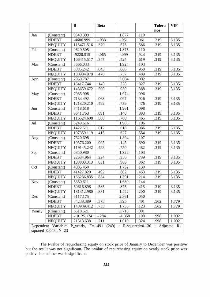
135
B Beta Tolera
nce
VIF
Jan (Constant) 9549.399 1.877 .110
NDEBT -4686.999 -.033 -.051 .961 .319 3.135
NEQUITY 115471.516 .379 .575 .586 .319 3.135
Feb (Constant) 9629.505 1.875 .110
NDEBT -9220.515 -.065 -.099 .924 .319 3.135
NEQUITY 106415.517 .347 .525 .619 .319 3.135
Mar (Constant) 8666.033 1.925 .103
NDEBT 5385.242 .043 .066 .950 .319 3.135
NEQUITY 130984.979 .478 .737 .489 .319 3.135
Apr (Constant) 7950.787 2.004 .092
NDEBT 16417.744 .145 .228 .827 .319 3.135
NEQUITY 145659.672 .590 .930 .388 .319 3.135
May (Constant) 7985.908 1.974 .096
NDEBT 7134.492 .063 .097 .926 .319 3.135
NEQUITY 121320.210 .492 .759 .476 .319 3.135
Jun (Constant) 7418.618 1.961 .098
NDEBT 9641.753 .091 .140 .893 .319 3.135
NEQUITY 116524.608 .508 .780 .465 .319 3.135
Jul (Constant) 8249.616 1.903 .106
NDEBT 1422.511 .012 .018 .986 .319 3.135
NEQUITY 107359.119 .415 .627 .554 .319 3.135
Aug (Constant) 7620.698 1.894 .107
NDEBT 10576.200 .095 .145 .890 .319 3.135
NEQUITY 119145.242 .493 .750 .482 .319 3.135
Sep (Constant) 6850.980 1.922 .103
NDEBT 22634.964 .224 .350 .739 .319 3.135
NEQUITY 138803.313 .631 .986 .362 .319 3.135
Oct (Constant) 4985.450 1.752 .130
NDEBT 41427.820 .492 .802 .453 .319 3.135
NEQUITY 156236.835 .854 1.391 .214 .319 3.135
Nov (Constant) 5350.611 1.680 .144
NDEBT 50616.898 .535 .875 .415 .319 3.135
NEQUITY 181312.980 .881 1.442 .200 .319 3.135
Dec (Constant) 6117.175 2.361 .050
NDEBT 34238.389 .373 .895 .401 .562 1.779
NEQUITY 148939.412 .733 1.755 .123 .562 1.779
Yearly (Constant) 6510.521 3.710 .001
NDEBT -10125.124 -.284 -1.358 .190 .998 1.002
NEQUITY 21513.638 .211 1.010 .324 .998 1.002
Dependent Variable: P_yearly, F=1.491 (249) ; R-squared=0.130 ; Adjusted R-
squared=0.043 ; N=23
The t-value of repurchasing equity on stock price of January to December was positive
but the result was not significant. The t-value of repurchasing equity on yearly stock price was
positive but neither was it significant.
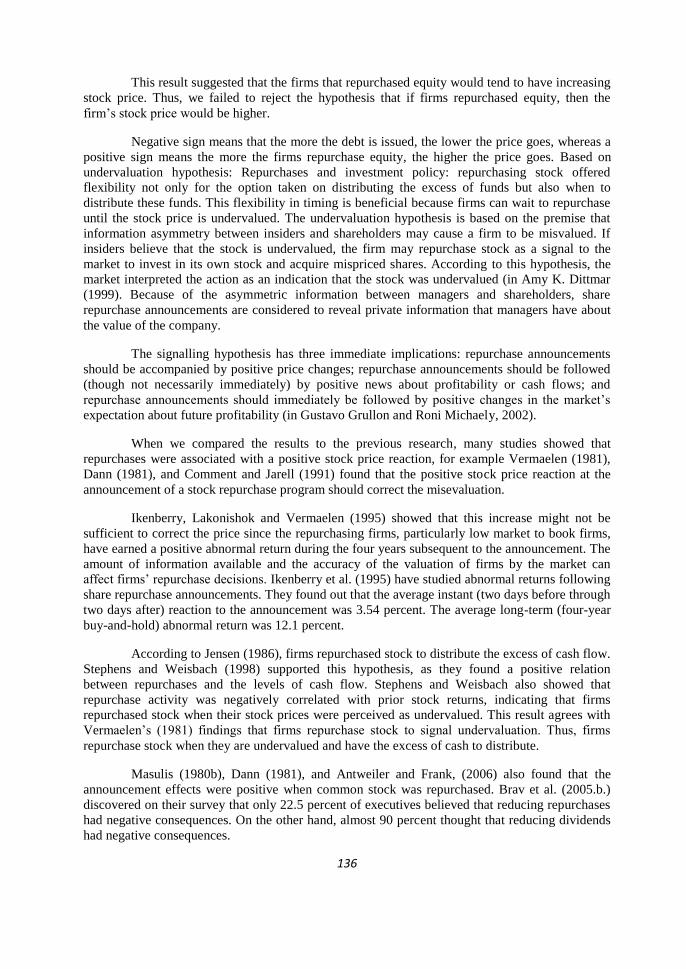
136
This result suggested that the firms that repurchased equity would tend to have increasing
stock price. Thus, we failed to reject the hypothesis that if firms repurchased equity, then the
firm‟s stock price would be higher.
Negative sign means that the more the debt is issued, the lower the price goes, whereas a
positive sign means the more the firms repurchase equity, the higher the price goes. Based on
undervaluation hypothesis: Repurchases and investment policy: repurchasing stock offered
flexibility not only for the option taken on distributing the excess of funds but also when to
distribute these funds. This flexibility in timing is beneficial because firms can wait to repurchase
until the stock price is undervalued. The undervaluation hypothesis is based on the premise that
information asymmetry between insiders and shareholders may cause a firm to be misvalued. If
insiders believe that the stock is undervalued, the firm may repurchase stock as a signal to the
market to invest in its own stock and acquire mispriced shares. According to this hypothesis, the
market interpreted the action as an indication that the stock was undervalued (in Amy K. Dittmar
(1999). Because of the asymmetric information between managers and shareholders, share
repurchase announcements are considered to reveal private information that managers have about
the value of the company.
The signalling hypothesis has three immediate implications: repurchase announcements
should be accompanied by positive price changes; repurchase announcements should be followed
(though not necessarily immediately) by positive news about profitability or cash flows; and
repurchase announcements should immediately be followed by positive changes in the market‟s
expectation about future profitability (in Gustavo Grullon and Roni Michaely, 2002).
When we compared the results to the previous research, many studies showed that
repurchases were associated with a positive stock price reaction, for example Vermaelen (1981),
Dann (1981), and Comment and Jarell (1991) found that the positive stock price reaction at the
announcement of a stock repurchase program should correct the misevaluation.
Ikenberry, Lakonishok and Vermaelen (1995) showed that this increase might not be
sufficient to correct the price since the repurchasing firms, particularly low market to book firms,
have earned a positive abnormal return during the four years subsequent to the announcement. The
amount of information available and the accuracy of the valuation of firms by the market can
affect firms‟ repurchase decisions. Ikenberry et al. (1995) have studied abnormal returns following
share repurchase announcements. They found out that the average instant (two days before through
two days after) reaction to the announcement was 3.54 percent. The average long-term (four-year
buy-and-hold) abnormal return was 12.1 percent.
According to Jensen (1986), firms repurchased stock to distribute the excess of cash flow.
Stephens and Weisbach (1998) supported this hypothesis, as they found a positive relation
between repurchases and the levels of cash flow. Stephens and Weisbach also showed that
repurchase activity was negatively correlated with prior stock returns, indicating that firms
repurchased stock when their stock prices were perceived as undervalued. This result agrees with
Vermaelen‟s (1981) findings that firms repurchase stock to signal undervaluation. Thus, firms
repurchase stock when they are undervalued and have the excess of cash to distribute.
Masulis (1980b), Dann (1981), and Antweiler and Frank, (2006) also found that the
announcement effects were positive when common stock was repurchased. Brav et al. (2005.b.)
discovered on their survey that only 22.5 percent of executives believed that reducing repurchases
had negative consequences. On the other hand, almost 90 percent thought that reducing dividends
had negative consequences.
137
Overall, our result is in line with the signalling hypothesis that has immediate
implications: repurchase announcements should be accompanied by positive price changes. It is
also consistent with many empirical evidences.
6.3.4.2 Analysis of the Indonesian Condition
In Indonesia, why can the stock price go up and down? Stock price movements are
determined by supply and demand for these shares. Demand increases, the stock price increases
and vice versa. Factors that affect stock price movements include the movements in interest rates,
inflation, exchange rate of the Rupiah, performance of the company such as sales and profit
increases, for dividends and so on. Non-economic factors including social and political conditions
also influenced the firm‟s stock price.
Stock price movements are determined by the issue of equity and debt. Firms in the
manufacturing sector of the LQ45 Index take the advantages of debt compared to equity. Issuance
of debt has a tax benefit because of the debt tax shield. A company with a higher tax rate thus has
a higher tax benefit from debt issuance. Some assert that debt adds discipline to management
because interest expenses cause lower cash flows, which makes management more likely to be
efficient. Hence, debt issue has positive effect on stock price.
Meanwhile, firms in the manufacturing sector of the LQ45 Index face the problems
because of increasing using leverage, even though the firms have high asset tangibility to secure
their debt. The firms have a risk of bankruptcy. Additionally, unlike equity, debt must at some
point be repaid. High interest costs during difficult financial periods can increase the risk of
insolvency, and companies that are too highly leveraged (that have large amounts of debt as
compared to equity) often find it difficult to grow because of the high cost of servicing the debt.
Therefore, our result shows that the positive influence of debt issue on stock price is not
significant.
6.4. Research Question 4, Hypothesis, Hypothesis Testing, and Result Analysis
In this study, the research question, hypothesis, hypothesis testing, and result analysis four are
explained in the follow sub-sections:
6.4.1. Research Question 4
Our research question 4 is, in the context of firm‟s life cycle, can we expect that growth [and
small] firms follow the pecking order theory more closely than mature [and large] firms?
6.4.2. Hypothesis 4
As our hypothesis 4 state that, in the context of a firm‟s life cycle, we expect that growth [and
small] firms follow the pecking order theory more closely than mature [and large] firms, hence, we
test this hypothesis applying multiple regression and augmented analysis as in hypothesis 2, but in
the context of firm‟s life cycle.
6.4.3. Testing Hypothesis 4
As described in chapter 5, multiple regression analysis and augmented analysis were
selected to test hypothesis 4. For testing hypothesis 4, the independent variable was financing
deficit and net debt issue and net equity issue, were the dependent variables.
The objective of regression analysis is to examine which firm is more following the
pecking order theory, growth firms or mature firms. If firms followed the pecking order theory, the
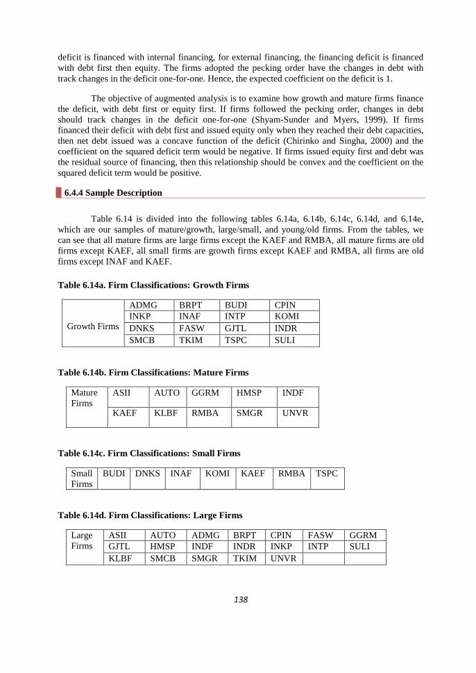
138
deficit is financed with internal financing, for external financing, the financing deficit is financed
with debt first then equity. The firms adopted the pecking order have the changes in debt with
track changes in the deficit one-for-one. Hence, the expected coefficient on the deficit is 1.
The objective of augmented analysis is to examine how growth and mature firms finance
the deficit, with debt first or equity first. If firms followed the pecking order, changes in debt
should track changes in the deficit one-for-one (Shyam-Sunder and Myers, 1999). If firms
financed their deficit with debt first and issued equity only when they reached their debt capacities,
then net debt issued was a concave function of the deficit (Chirinko and Singha, 2000) and the
coefficient on the squared deficit term would be negative. If firms issued equity first and debt was
the residual source of financing, then this relationship should be convex and the coefficient on the
squared deficit term would be positive.
6.4.4 Sample Description
Table 6.14 is divided into the following tables 6.14a, 6.14b, 6.14c, 6.14d, and 6.14e,
which are our samples of mature/growth, large/small, and young/old firms. From the tables, we
can see that all mature firms are large firms except the KAEF and RMBA, all mature firms are old
firms except KAEF, all small firms are growth firms except KAEF and RMBA, all firms are old
firms except INAF and KAEF.
Table 6.14a. Firm Classifications: Growth Firms
Growth Firms
ADMG BRPT BUDI CPIN
INKP INAF INTP KOMI
DNKS FASW GJTL INDR
SMCB TKIM TSPC SULI
Table 6.14b. Firm Classifications: Mature Firms
Mature
Firms
ASII AUTO GGRM HMSP INDF
KAEF KLBF RMBA SMGR UNVR
Table 6.14c. Firm Classifications: Small Firms
Small
Firms
BUDI DNKS INAF KOMI KAEF RMBA TSPC
Table 6.14d. Firm Classifications: Large Firms
Large
Firms
ASII AUTO ADMG BRPT CPIN FASW GGRM
GJTL HMSP INDF INDR INKP INTP SULI
KLBF SMCB SMGR TKIM UNVR

139
Table 6.14e. Firm Classifications: Old and Young Firms
Old Firms ASII AUTO ADMG BRPT CPIN FASW GGRM GJTL
BUDI DNKS INDR INKP INTP KLBF KOMI RMBA
TKIM TSPC UNVR SULI SMCB SMGR HMSP INDF
Young
Firms
INAF KAEF
Bulan, Subramanian, and Tanlu (2007) found that firms that initiated dividends were
mature firms. Thus, Bulan and Yan (2007) identified firms in their mature stage by their dividend
history. By following Bulan and Yan (2007) to construct the growth and mature sample firms, to
deem the 6-year dividends payment periods as the mature stage of a firm‟s life cycle, we found 10
firms which have one 6-year dividend payment period; while 16 firms have less than one 6-year
dividend payment periods.
Meanwhile, 8 of our 10 mature firms are large firms, except KAEF, RMBA. KAEF went
public on July 4, 2001. Its amount of total assets made KAEF was categorised as a small firm
(Hufft, JR category). It was established on January 23, 1969 and the firm was a dividend payer.
Based on those facts, KAEF is a small young mature firm that is liquid enough to pay dividend to
the shareholder. RMBA is a small mature old firm that pays dividend for 6 years consecutively
(Bulan and Yan, 2007).
We have 7 small firms and 19 large firms based on the Hufft category with total assets of
less than $150 million, or equal to IDR 1,081,028.68 - 1,086,876.61 million. Our sample of firms
which were categorised into young firms, based on Evans (1987) who defined firms of six years
old or younger as young firms and firms of seven years or older as old firms, were INAF and
KAEF. INAF was established on January 2, 1996 and went public on April 17, 2001. INAF is also
a small-growth firm. KAEF was established on January 23, 1969 and went public on July 4, 2001.
INAF is a small-mature firm.
6.4.5. Analysis of Results
The following sub-sections are analysis of results for growth and mature firms and its consistency
with the theory and previous research, and also with the Indonesian capital market condition.
6.4.5.1 Analysis of Results and Its Consistency to the Theory and Previous Research
(Growth and Mature Firms)
As shown by table 6.15-6.16, the regression result for mature and growth firms are as follow: The
financing deficit is financed with debt and/or equity. If firms follow the pecking order, changes in
debt should track changes in the deficit one-for-one. Therefore, the expected coefficient on the
deficit is 1.
Table 6.15. Regression and Augmented Results for Mature Firms
Coefficientsa
Model Unstandardised
Coefficients
Standar
dised Co-
efficients
t Sig. Collinearity
Statistics
B Std.
Error
Beta Tolera
nce
VIF
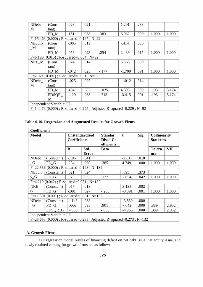
140
NDebt_
M
(Cons
tant)
.026 .021 1.201 .233
FD_M .151 .038 .383 3.932 .000 1.000 1.000
F=15.463 (0.000) ; R-squared=0.147 ; N=92
NEquity
_M
(Cons
tant)
-.005 .013 -.414 .680
FD_M .058 .023 .254 2.489 .015 1.000 1.000
F=6.196 (0.015) ; R-squared=0.064 ; N=92
NRE_M (Cons
tant)
.074 .014 5.368 .000
FD_M -.042 .025 -.177 -1.709 .091 1.000 1.000
F=2.921 (0.091) ; R-squared=0.031 ; N=92
NDebt_
M
(Cons
tant)
-.025 .025 -1.012 .314
FD_M .404 .082 1.025 4.895 .000 .193 5.174
FDSQR_
M
-.129 .038 -.715 -3.415 .001 .193 5.174
Independent Variable: FD
F=14.478 (0.000) ; R-squared=0.245 ; Adjusted R-squared=0.229 ; N=92
Table 6.16. Regression and Augmented Results for Growth Firms
Coefficients
Model Unstandardised
Coefficients
Standar
Dised Co-
efficients
t Sig. Collinearity
Statistics
B Std.
Error
Beta Tolera
nce
VIF
NDebt
_G
(Constant) -.106 .041 -2.617 .010
FD_G .284 .060 .385 4.749 .000 1.000 1.000
F=22.556 (0.000) ; R-squared=0.148 ; N=132
NEquit
y_G
(Constant) .021 .024 .895 .373
FD_G .073 .035 .177 2.054 .042 1.000 1.000
F=4.219 (0.042) ; R-squared=0.031 ; N=132
NRE_
G
(Constant) .057 .018 3.135 .002
FD_G -.091 .027 -.285 -3.391 .001 1.000 1.000
F=11.501 (0.001) ; R-squared=0.081 ; N=132
NDebt
_G
(Constant) -.146 .038 -3.830 .000
FD_G .666 .095 .901 7.042 .000 .339 2.952
FDSQR_G -.365 .074 -.635 -4.965 .000 .339 2.952
Independent Variable: FD
F=25.653 (0.000) ; R-squared=0.285 ; Adjusted R-squared=0.273 ; N=132
A. Growth Firms
Our regression model results of financing deficit on net debt issue, net equity issue, and
newly retained earning for growth firms are as follow:

141
Regression Model Result
In the regression model, Y is net debt issued and deficit is the financing deficit. This
deficit is financed with debt and/or equity. If firms follow the pecking order, changes in debt
should track changes in the deficit one-for-one. Therefore, the expected coefficient on the deficit
is 1.
Net Debt Issue
From the tables we can conclude that the financing deficit has positive significant effects
on net debt issue with t-value of 4.749 (it higher than mature firms) and significance value of
0.000. This result suggests that high deficit firms would tend to issue more net debt. However, the
coefficient on the deficit is 0.284 and constant value is -0.106.
Net Equity Issue
The financing deficit has positive but not significant effects on net equity issue with t-
value of 2.054 (it lower than mature firms) and significance value of 0.042. This result suggests
that high deficit firms would tend to issue more net equity. However, the coefficient on the deficit
is 0.073 and the constant value is 0.021.
Newly Retained Earning
The financing deficit has negative significant effects on newly retained earning with t-
value of -3.391 (it more negative than mature firms) and significance value of 0.001. This result
suggests that high deficit firms would not tend to use newly retained earning. However, the
coefficient on the deficit is -0.091 and constant value is 0.057.
Augmented Model Result
If firms are issuing equity first and debt is the residual source of financing, then this
relationship should be convex and the coefficient on the squared deficit term would be positive.
However, our result shows a negative coefficient on the squared deficit term, it implies that firms
are limited by their debt capacity constraints and they have to resort to issuing equity. A squared
deficit coefficient that is large in absolute value implies a greater reliance on equity finance for
larger values of the financing deficit.
From these results, we can conclude that our sample of growth firm in the manufacturing
sector of the LQ45 Index prefers external to internal financing and debt to equity if external
financing is used. This is consistent with the theory‟s prediction that firms with the greatest
information asymmetry problems (specifically young, growth firms) are precisely those that
should be making financing choices according to the pecking order. Growth firms in the
manufacturing sector of the LQ45 Index should face more asymmetric information in capital
markets and be less watched by the analysts.
B. Mature Firms
Our regression model results of financing deficit on net debt issue, net equity issue, and
newly retained earning for mature firms are as follow.
Regression Model Result
142
As for growth firms, the regression model of mature firms, Y is net debt issued and
deficit is the financing deficit. This deficit is financed with debt and/or equity. If firms follow the
pecking order, changes in debt should track changes in the deficit one-for-one. Therefore, the
expected coefficient on the deficit is 1.
Net Debt Issue
From the tables we can conclude that the financing deficit has positive significant effects
on net debt issue with t-value of 3.932 and significance value of 0.000. This result suggests that
high deficit firms would tend to issue more net debt. However, the coefficient on the deficit is
0.151 and constant value is 0.026.
Net Equity Issue
The financing deficit has positive significant effects on net equity issue with t-value of
2.489 and significance value of 0.015. This result suggests that high deficit firms would tend to
issue more net equity. However, the coefficient on the deficit is 0.058 and the constant value is -
0.005.
Newly Retained Earning
The financing deficit has negative significant effects on newly retained earning with t-
value of -1.709 and significance value of 0.091. This result suggests that high deficit firms would
not tend to use newly retained earning. However, the coefficient on the deficit is -0.042 and
constant value is 0.074.
Augmented Model Result
If firms are issuing equity first and debt is the residual source of financing, then this
relationship should be convex and the coefficient on the squared deficit term would be positive.
However, our result shows a negative coefficient on the squared deficit term, it implies that firms
are limited by their debt capacity constraints and they have to resort to issuing equity. A squared
deficit coefficient that is large in absolute value implies a greater reliance on equity finance for
larger values of the financing deficit.
Prefer External or Internal Financing?
The coefficient of financing deficit on newly retained earning is negative for growth and
mature firms. The coefficient of financing deficit on net debt and net equity issue are positive
significant for growth and mature firms. For both firms, the significance value of net debt issue is
more significant than net equity issue. The evidence seems to suggest mature and growth firms
rely more heavily on external financing.
Prefer Debt or Equity?
Growth firms have the same 0.000 significantly value with mature firms while growth
firms have higher standardised coefficients (0.385) of deficit on net debt issue than mature firms
(0.383), however mature firms have higher standardised coefficients (0.254) of deficit on net
equity issue than of growth firms (0.177). These results imply that deficit of mature firms is solved
more by net equity issue while deficit of growth firms is solved more by net debt issue.
143
From augmented model result, the findings are consistent with the firms following the
pecking order: the coefficient on the deficit is positive and the coefficient on the deficit-square is
negative. Both growth and mature firms are issuing debt first, while equity is the residual source of
financing once they reach their debt capacities. Our evidence seems to suggest mature and growth
firms rely more heavily on debt financing rather than equity financing.
For growth firms, Adjusted R Square (0.273) and R Square (0.285) are stronger than
mature firms (0.229) and (0.245). R-squared of financing deficit on net debt issue of growth firms
are higher than mature firms, while R-squared of financing deficit on net equity issue of mature
firms are higher than of growth firms. Therefore, overall, we find that the pecking order theory
describes the financing patterns of growth firms better than mature firms.
Adjusted R-squared of predictors of financing deficit and the financing deficit square on
net debt issue of growth firms (0.273) are higher than mature firms (0.229). It implies that
financing deficit and financing deficit square on net debt issue of growth firms rely more on net
debt issue. Therefore, the pecking order theory describes the financing patterns of growth firms
better than mature firms, as mature firms are more closely followed by analysts and are better
known to investors, and hence, should suffer less from problems of information asymmetry.
The results are consistent with firms following the pecking order: the coefficient on the
deficit is positive and the coefficient on the deficit square is negative. Both growth and mature
firms are issuing debt first, while equity is the residual source of financing once they reach their
debt capacities. Comparing across life cycle stages however, we found that growth firms have
significantly higher debt-deficit sensitivities indicating that growth firms follow the pecking order
more closely. This is consistent to conventional wisdom since they would expect growth firms to
suffer more from information asymmetry problems. This result is not in line with the finding
research of Bulan and Yan (2009).
Older and more mature firms are more closely followed by analysts and are better known
to investors, and hence, should suffer less from problems of information asymmetry. For example,
a good reputation (such as a long credit history) mitigates the adverse selection problem between
borrowers and lenders. Thus, mature firms are able to obtain better loan rates compared to their
younger firm counterparts (Diamond, 1989). Furthermore, mature firms generally have more
internal funds due to higher profitability and lower growth opportunities. Older, more stable and
highly profitable firms with few growth opportunities and good credit histories are more suited to
use internal funds first, and then debt before equity for their financing needs.
As explained by the pecking order theory, firms with the greatest information asymmetry
problems (specifically young growth firms) are precisely those that should be making financing
choices based on the pecking order. Thus, they are more suited to use internal funds first, and then
debt before equity for their financing needs.
From descriptive statistics and correlation matrix, we conclude that: growth firms have
lower newly retained earning and lower profitability. It is indicated by profitability and newly
retained earning which have positive significant correlation (0.654; 0.000). It suggests that the
larger the firm‟s profitability, the higher the firm‟s newly retained earning.
Small-growth firms issue more net debt to solve financing deficit than equity as they have
higher asset tangibility to secure net debt issue. It was shown by tangibility and financing deficit
have positive significant correlation (0.551; 0.000) which implies that firm that has higher

144
financing deficit has larger asset tangibility to secure debt issue. Tang and newly retained earning
are negative significant correlated (-0.227; 0.001), it implies that the lower the firm‟s newly
retained earning the larger the firm‟s tangibility.
However, growth-small firms have higher profitability than mature-large firms. It shown
by profitability and asset tangibility which have negative significant correlation and size and asset
tangibility have positive significant correlation, profitability and risk have negative significant
correlation. Hence, small-growth firms have low risk (earning volatility).
Even though growth firms have higher financing deficit, financing deficit square, net
equity issued, but they finance their financing deficit with more net debt issue than net equity
issue, while mature firms have higher net debt issued, but they manage their financing deficit with
more net equity issue than net debt issue.
For growth firms, long-term leverage and capital expenditure have higher composition in
forming financing deficit, while for mature firms dividend and working capital have higher
composition in forming financing deficit as mature firms have higher newly retained earning.
Mature firms have higher dividend, working capital, cashflow, newly retained earning,
net debt issued, while growth firms have higher long-term leverage, fixed asset, financing deficit,
financing deficit1square, net equity issued (descriptive statistics). Growth firms have lower
profitability, higher tangibility, higher risk, while mature firms have higher profitability, lower
tangibility, lower risk (correlation matrix).
It can be shown that there exists positive significant correlation (0.654; 0,000) between
profitability and newly retained earning. The larger the firm‟s profitability, the higher the firm‟s
newly retained earning.
Profitability and financing deficit are significantly negative (-0.461; 0.000). It suggests
that the larger the firm‟s profitability, the smaller the firm‟s financing deficit. Tangibilty and
financing deficit are significantly positive (0.551; 0.000). It implies that the larger the firm‟s
tangibility, the higher the firm‟s financing deficit. Tangibility and newly retained earning are
significantly negative (-0.227; 0.001). It implies that the larger the firm‟s tangibility, the lower the
firm‟s financing deficit. Risk and newly retained earning are significantly negative (-0.444; 0.000).
It implies that the larger the firm‟s risk, the lower the firm‟s newly retained earning.
According to Myers (1984), a firm is said to follow a pecking order if it prefers internal to
the external financing and debt to equity if external financing is used. Therefore, overall, we found
that the pecking order theory described the financing patterns of growth firms better than mature
firms, as mature firms were more closely followed by analysts and were better known to investors,
and hence, should suffer less from problems of information asymmetry. Our result is consistent
from the theory, and also consistent from the previous research findings of Shyam-Sunder and
Myers (1999). They proposed a direct test of the pecking order and found strong support for the
theory among a sample of large firms.
However, some empirical evidence for the pecking order theory over firms life cycles
which are inconsistent with our results are as follow: The plausible explanation is that the
Indonesian economy and market conditions differ from those under which the previous research
was developed, such as the USA.
More recent work by Lemmon and Zender (2004) and Agca and Mozumdar (2004) have
shown that the Shyam-Sunder and Myers test did not account for a firm‟s debt capacity; a

145
constraint that was particularly binding for small firms. Thus, it was not surprising that this test
failed to find support for the pecking order among small firms. To address this shortcoming,
Lemmon and Zender and Agca and Mozumdar used sub-samples of firms that were the least debt-
constrained and they found support for the pecking order. In addition, once debt capacity
constraints were accounted for, they found that the pecking order performed well even for small
firms.
Frank and Goyal (2003), found that large firms fitted the pecking order theory better than
of small firms, contrary to the predictions of the theory. Frank and Goyal (2003) examined the
broad applicability of the pecking order theory. Their evidence was based on a large cross-section
of US publicly traded firms over long time periods. It showed that external financing was heavily
used by some firms. On average net equity issued track the financing deficit more closely than did
net debt issues. These facts did not match the claims of the pecking order theory. The greatest
support for pecking order was found among large firms, which might be expected to face the least
severe adverse selection problem since they received much better coverage by equity analysts.
Even here, the support for pecking order was declining over time and the support for pecking order
among large firms was weaker in the 1990s. They concluded that the pecking order theory did not
explain broad patterns in the data.
Overall, Bulan and Yan (2007) found that the pecking order theory described the
financing patterns of mature firms better than of growth firms. This is contrary to the theory‟s
prediction that firms with the greatest information asymmetry problems (specifically young,
growth firms) are precisely those that should be making financing choices according to the
pecking order. These results are robust under alternative empirical models for testing the pecking
order theory.
Bulan and Yan (2007) further saw that growth firms had larger financing deficits, as
expected. The financing deficit is defined as the uses of funds minus internal sources of funds,
which, by an accounting identity, is also the sum of net debt issued and net equity issued. There
seems to be no difference in net debt issued between the two cohorts, while net equity issued is
larger for the growth firms. From this simple comparison, the evidence seems to suggest growth
firms rely more heavily on equity financing rather than debt. This finding is consistent with Agca
and Mozumdar (2004) and Lemmon and Zender (2004).
Bulan and Yan (2009) examined the central prediction of the pecking order theory of
financing among firms in two distinct life cycle stages, namely growth and maturity. They found
that within a life cycle stage, where levels of debt capacity and external financing needs were more
homogeneous, and after sufficiently controlling for debt capacity constraints, firms with high
adverse selection costs followed the pecking order more closely.
Financing deficit of growth firms are higher than financing deficit of mature firms, as
growth firms have lower cashflow than mature firms. Additionally, the findings that growth firms
had greater financing deficits but smaller debt capacities are implying that growth firms would
reach their debt capacities more often than mature firms.
The results are consistent with firms following the pecking order: the coefficient on the
deficit is positive and the coefficient on the deficit square is negative. Both growth and mature
firms issued debt first, while equity is the residual source of financing once they reach their debt
capacities. Comparing across life cycle stages however, they found that mature firms had
significantly higher debt-deficit sensitivities indicating that mature firms followed the pecking
order more closely. That was contrary to conventional wisdom, since they would expect growth
firms to suffer more from information asymmetry problems. Bulan and Yan (2009) documented
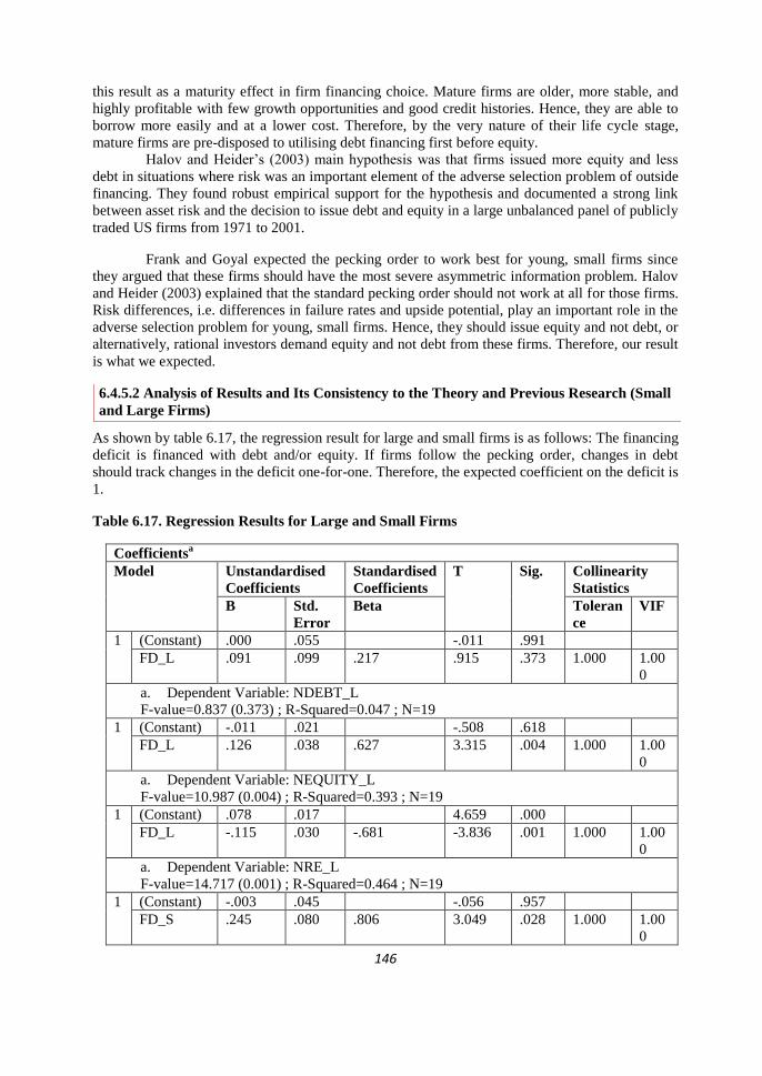
146
this result as a maturity effect in firm financing choice. Mature firms are older, more stable, and
highly profitable with few growth opportunities and good credit histories. Hence, they are able to
borrow more easily and at a lower cost. Therefore, by the very nature of their life cycle stage,
mature firms are pre-disposed to utilising debt financing first before equity.
Halov and Heider‟s (2003) main hypothesis was that firms issued more equity and less
debt in situations where risk was an important element of the adverse selection problem of outside
financing. They found robust empirical support for the hypothesis and documented a strong link
between asset risk and the decision to issue debt and equity in a large unbalanced panel of publicly
traded US firms from 1971 to 2001.
Frank and Goyal expected the pecking order to work best for young, small firms since
they argued that these firms should have the most severe asymmetric information problem. Halov
and Heider (2003) explained that the standard pecking order should not work at all for those firms.
Risk differences, i.e. differences in failure rates and upside potential, play an important role in the
adverse selection problem for young, small firms. Hence, they should issue equity and not debt, or
alternatively, rational investors demand equity and not debt from these firms. Therefore, our result
is what we expected.
6.4.5.2 Analysis of Results and Its Consistency to the Theory and Previous Research (Small
and Large Firms)
As shown by table 6.17, the regression result for large and small firms is as follows: The financing
deficit is financed with debt and/or equity. If firms follow the pecking order, changes in debt
should track changes in the deficit one-for-one. Therefore, the expected coefficient on the deficit is
1.
Table 6.17. Regression Results for Large and Small Firms
Coefficientsa
Model Unstandardised
Coefficients
Standardised
Coefficients
T Sig. Collinearity
Statistics
B Std.
Error
Beta Toleran
ce
VIF
1 (Constant) .000 .055 -.011 .991
FD_L .091 .099 .217 .915 .373 1.000 1.00
0
a. Dependent Variable: NDEBT_L
F-value=0.837 (0.373) ; R-Squared=0.047 ; N=19
1 (Constant) -.011 .021 -.508 .618
FD_L .126 .038 .627 3.315 .004 1.000 1.00
0
a. Dependent Variable: NEQUITY_L
F-value=10.987 (0.004) ; R-Squared=0.393 ; N=19
1 (Constant) .078 .017 4.659 .000
FD_L -.115 .030 -.681 -3.836 .001 1.000 1.00
0
a. Dependent Variable: NRE_L
F-value=14.717 (0.001) ; R-Squared=0.464 ; N=19
1 (Constant) -.003 .045 -.056 .957
FD_S .245 .080 .806 3.049 .028 1.000 1.00
0
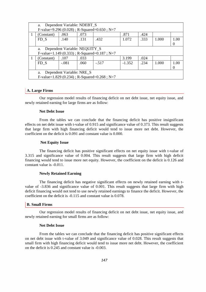
147
a. Dependent Variable: NDEBT_S
F-value=9.296 (0.028) ; R-Squared=0.650 ; N=7
1 (Constant) .063 .073 .871 .424
FD_S .140 .131 .432 1.072 .333 1.000 1.00
0
a. Dependent Variable: NEQUITY_S
F-value=1.149 (0.333) ; R-Squared=0.187 ; N=7
1 (Constant) .107 .033 3.199 .024
FD_S -.081 .060 -.517 -1.352 .234 1.000 1.00
0
a. Dependent Variable: NRE_S
F-value=1.829 (0.234) ; R-Squared=0.268 ; N=7
A. Large Firms
Our regression model results of financing deficit on net debt issue, net equity issue, and
newly retained earning for large firms are as follow:
Net Debt Issue
From the tables we can conclude that the financing deficit has positive insignificant
effects on net debt issue with t-value of 0.915 and significance value of 0.373. This result suggests
that large firm with high financing deficit would tend to issue more net debt. However, the
coefficient on the deficit is 0.091 and constant value is 0.000.
Net Equity Issue
The financing deficit has positive significant effects on net equity issue with t-value of
3.315 and significance value of 0.004. This result suggests that large firm with high deficit
financing would tend to issue more net equity. However, the coefficient on the deficit is 0.126 and
constant value is -0.011.
Newly Retained Earning
The financing deficit has negative significant effects on newly retained earning with t-
value of -3.836 and significance value of 0.001. This result suggests that large firm with high
deficit financing would not tend to use newly retained earnings to finance the deficit. However, the
coefficient on the deficit is -0.115 and constant value is 0.078.
B. Small Firms
Our regression model results of financing deficit on net debt issue, net equity issue, and
newly retained earning for small firms are as follow:
Net Debt Issue
From the tables we can conclude that the financing deficit has positive significant effects
on net debt issue with t-value of 3.049 and significance value of 0.028. This result suggests that
small firm with high financing deficit would tend to issue more net debt. However, the coefficient
on the deficit is 0.245 and constant value is -0.003.
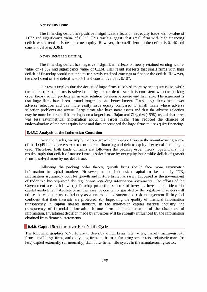
148
Net Equity Issue
The financing deficit has positive insignificant effects on net equity issue with t-value of
1.072 and significance value of 0.333. This result suggests that small firm with high financing
deficit would tend to issue more net equity. However, the coefficient on the deficit is 0.140 and
constant value is 0.063.
Newly Retained Earning
The financing deficit has negative insignificant effects on newly retained earning with t-
value of -1.352 and significance value of 0.234. This result suggests that small firms with high
deficit of financing would not tend to use newly retained earnings to finance the deficit. However,
the coefficient on the deficit is -0.081 and constant value is 0.107.
Our result implies that the deficit of large firms is solved more by net equity issue, while
the deficit of small firms is solved more by the net debt issue. It is consistent with the pecking
order theory which predicts an inverse relation between leverage and firm size. The argument is
that large firms have been around longer and are better known. Thus, large firms face lower
adverse selection and can more easily issue equity compared to small firms where adverse
selection problems are severe. Large firms also have more assets and thus the adverse selection
may be more important if it impinges on a larger base. Rajan and Zingales (1995) argued that there
was less asymmetrical information about the larger firms. This reduced the chances of
undervaluation of the new equity issue and thus encouraged the large firms to use equity financing.
6.4.5.3 Analysis of the Indonesian Condition
From the results, we imply that our growth and mature firms in the manufacturing sector
of the LQ45 Index prefers external to internal financing and debt to equity if external financing is
used. Therefore, both kinds of firms are following the pecking order theory. Specifically, the
results imply that deficit of mature firms is solved more by net equity issue while deficit of growth
firms is solved more by net debt issue.
Following the pecking order theory, growth firms should face more asymmetric
information in capital markets. However, in the Indonesian capital market namely IDX,
information asymmetry both for growth and mature firms has rarely happened as the government
of Indonesia has stipulated the regulations regarding information asymmetry. The efforts of the
Government are as follow: (a) Develop protection scheme of investor. Investor confidence in
capital markets is in absolute terms that must be constantly guarded by the regulator. Investors will
utilise the capital markets industry as a means of investment and risk management if they feel
confident that their interests are protected. (b) Improving the quality of financial information
transparency in capital market industry. In the Indonesian capital markets industry, the
transparency of financial information is one form of implementation of the disclosure of
information. Investment decision made by investors will be strongly influenced by the information
obtained from financial statements.
6.4.6. Capital Structure over Firm’s Life Cycle
The following graphics 6.7-6.16 are to describe which firms‟ life cycles, namely mature/growth
firms, small/large firms, and old/young firms in the manufacturing sector raise relatively more (or
less) capital externally (or internally) than other firms‟ life cycles in the manufacturing sector.
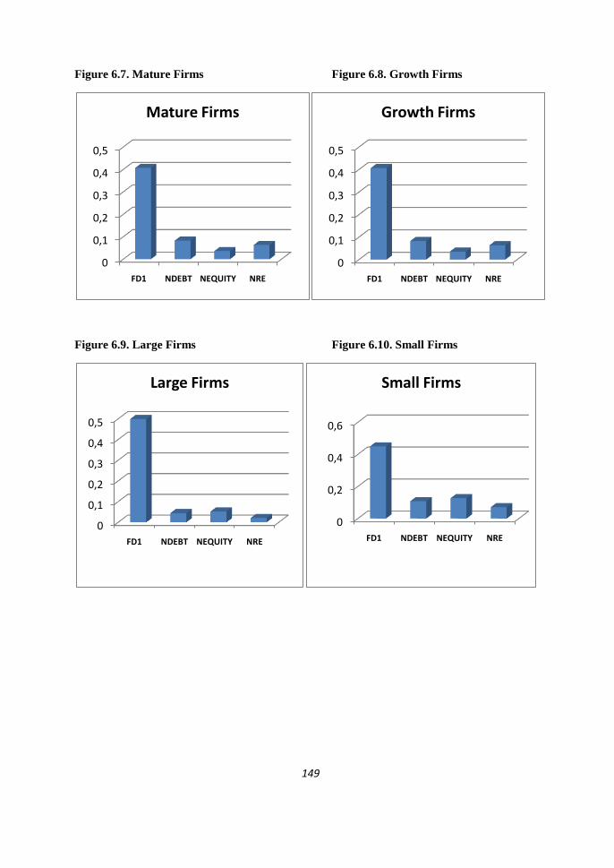
149
Figure 6.7. Mature Firms Figure 6.8. Growth Firms
Figure 6.9. Large Firms Figure 6.10. Small Firms
0
0,1
0,2
0,3
0,4
0,5
FD1 NDEBT NEQUITY NRE
Mature Firms
0
0,1
0,2
0,3
0,4
0,5
FD1 NDEBT NEQUITY NRE
Growth Firms
0
0,1
0,2
0,3
0,4
0,5
FD1 NDEBT NEQUITY NRE
Large Firms
0
0,2
0,4
0,6
FD1 NDEBT NEQUITY NRE
Small Firms
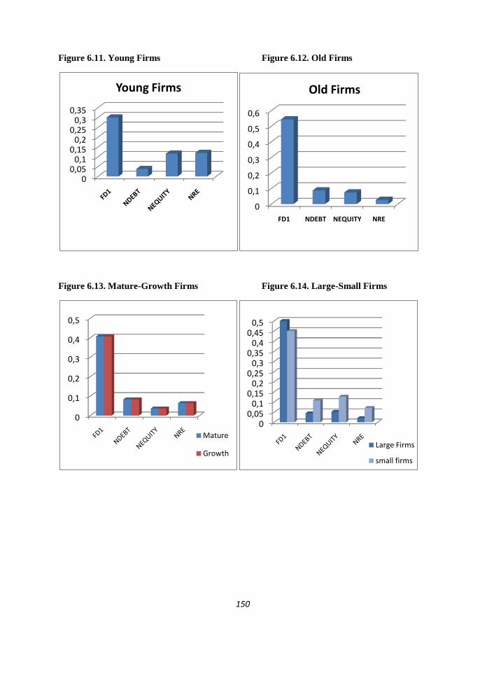
150
Figure 6.11. Young Firms Figure 6.12. Old Firms
Figure 6.13. Mature-Growth Firms Figure 6.14. Large-Small Firms
00,05
0,10,15
0,20,25
0,30,35
Young Firms
0
0,1
0,2
0,3
0,4
0,5
0,6
FD1 NDEBT NEQUITY NRE
Old Firms
0
0,1
0,2
0,3
0,4
0,5
Mature
Growth
00,05
0,10,15
0,20,25
0,30,35
0,40,45
0,5
Large Firms
small firms
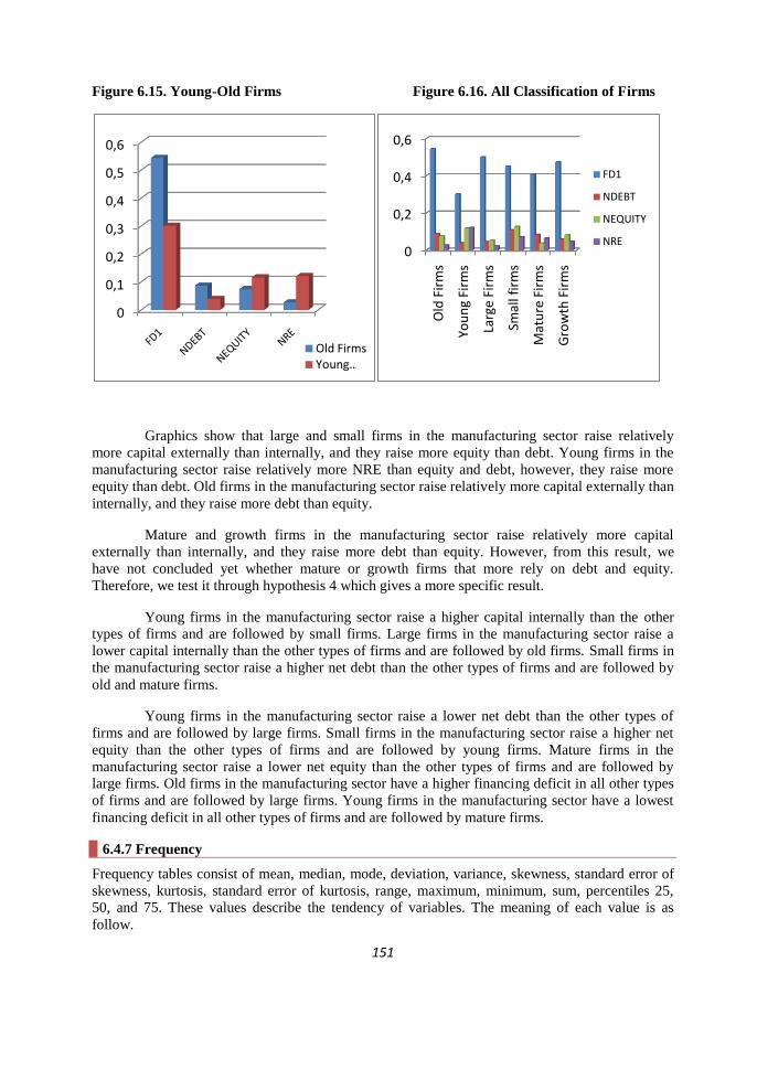
151
Figure 6.15. Young-Old Firms Figure 6.16. All Classification of Firms
Graphics show that large and small firms in the manufacturing sector raise relatively
more capital externally than internally, and they raise more equity than debt. Young firms in the
manufacturing sector raise relatively more NRE than equity and debt, however, they raise more
equity than debt. Old firms in the manufacturing sector raise relatively more capital externally than
internally, and they raise more debt than equity.
Mature and growth firms in the manufacturing sector raise relatively more capital
externally than internally, and they raise more debt than equity. However, from this result, we
have not concluded yet whether mature or growth firms that more rely on debt and equity.
Therefore, we test it through hypothesis 4 which gives a more specific result.
Young firms in the manufacturing sector raise a higher capital internally than the other
types of firms and are followed by small firms. Large firms in the manufacturing sector raise a
lower capital internally than the other types of firms and are followed by old firms. Small firms in
the manufacturing sector raise a higher net debt than the other types of firms and are followed by
old and mature firms.
Young firms in the manufacturing sector raise a lower net debt than the other types of
firms and are followed by large firms. Small firms in the manufacturing sector raise a higher net
equity than the other types of firms and are followed by young firms. Mature firms in the
manufacturing sector raise a lower net equity than the other types of firms and are followed by
large firms. Old firms in the manufacturing sector have a higher financing deficit in all other types
of firms and are followed by large firms. Young firms in the manufacturing sector have a lowest
financing deficit in all other types of firms and are followed by mature firms.
6.4.7 Frequency
Frequency tables consist of mean, median, mode, deviation, variance, skewness, standard error of
skewness, kurtosis, standard error of kurtosis, range, maximum, minimum, sum, percentiles 25,
50, and 75. These values describe the tendency of variables. The meaning of each value is as
follow.
0
0,1
0,2
0,3
0,4
0,5
0,6
Old FirmsYoung …
0
0,2
0,4
0,6
Old
Fir
ms
You
ng
Firm
s
Larg
e Fi
rms
Smal
l fir
ms
Mat
ure
Fir
ms
Gro
wth
Fir
ms
FD1
NDEBT
NEQUITY
NRE

152
The mode of a set of data values is the value (s) that occurs most often. The median of a
set of data values is the middle value of the data set when it has been arranged in ascending order.
That is, from the smallest value to the highest value. The mean (or average) of a set of data values
is the sum of all of the data values divided by the number of data values. Standard deviation is a
widely used measurement of variability or diversity used in statistics. It shows how much variation
or "dispersion" there is from the average (mean, or expected value). A low standard deviation
indicates that the data points tend to be very close to the mean, whereas high standard deviation
indicates that the data are spread out over a large range of values. In descriptive statistics, the
range is the length of the smallest interval which contains all the data. It is calculated by
subtracting the smallest observation (sample minimum) from the greatest (sample maximum) and
provides an indication of statistical dispersion. The variance is used as a measure of how far a set
of numbers are spread out from each other. It is one of several descriptors of a probability
distribution, describing how far the numbers lie from the mean (expected value). Skewness is a
measure of the asymmetry of the probability distribution of a real-valued random variable. The
skewness value can be positive or negative, or even undefined. Qualitatively, a negative skew
indicates that the tail on the left side of the probability density function is longer than the right side
and the bulk of the values (possibly including the median) lie to the right of the mean. A positive
skew indicates that the tail on the right side is longer than the left side and the bulk of the values
lie to the left of the mean. A zero value indicates that the values are relatively evenly distributed
on both sides of the mean, typically but not necessarily implying a symmetric distribution.
Kurtosis is a measure of the "peakedness" of the probability distribution of a real-valued random
variable, although some sources are insistent that heavy tails, and not peakedness, is what is really
being measured by kurtosis. Higher kurtosis means more of the variance is the result of infrequent
extreme deviations, as opposed to frequent modestly sized deviations. Sum is the amount of the
values. Minimum is the minimum value. Maximum is the maximum value.
Table 6.18, 6.19, 6.20, 6.21, 6.22, and 6.23 show the frequency of mature-growth, large-
small, and old-young firms which analyse the mean, median, mode, deviation, variance, skewness,
standard error of skewness, kurtosis, standard error of kurtosis, range, maximum, minimum, sum,
and percentiles 25, 50, and 75.
Table 6.18. Frequency of Mature Firms
FD_M NRE_M NEQUITY_M NDEBT_M
N Valid 75 71 71 71
Missing 43 47 47 47
Mean .362999 .063057 .012640 .086801
Median .227218 .058904 .000243 .043679
Mode -.1737a -.1641
a .0000 -.1788
a
Std. Deviation .4579992 .1047534 .0989413 .1716948
Variance .210 .011 .010 .029
Skewness 2.993 1.509 -1.819 1.023
Std. Error of
Skewness
.277 .285 .285 .285
Kurtosis 11.483 7.753 19.773 1.292
Std. Error of
Kurtosis
.548 .563 .563 .563
Range 2.8143 .7445 .9578 .8371
Minimum -.1737 -.1641 -.5690 -.1788
Maximum 2.6406 .5805 .3888 .6583
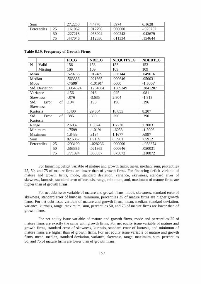
153
Sum 27.2250 4.4770 .8974 6.1628
Percentiles 25 .161062 .017796 .000000 -.025757
50 .227218 .058904 .000243 .043679
75 .447046 .112630 .011334 .154644
Table 6.19. Frequency of Growth Firms
FD_G NRE_G NEQUITY_G NDEBT_G
N Valid 156 153 153 153
Missing 106 109 109 109
Mean .529736 .012489 .056144 .049616
Median .563386 .021865 .000646 .050031
Mode -.7599a -1.0191
a .0000 -1.5006
a
Std. Deviation .3954524 .1254664 .1589349 .2841207
Variance .156 .016 .025 .081
Skewness -.076 -3.635 2.804 -1.913
Std. Error of
Skewness
.194 .196 .196 .196
Kurtosis 1.400 29.604 18.855 8.207
Std. Error of
Kurtosis
.386 .390 .390 .390
Range 2.6032 1.3324 1.7730 2.2003
Minimum -.7599 -1.0191 -.6053 -1.5006
Maximum 1.8433 .3134 1.1677 .6997
Sum 82.6387 1.9109 8.5901 7.5912
Percentiles 25 .293100 -.028236 .000000 -.058374
50 .563386 .021865 .000646 .050031
75 .771394 .068037 .075072 .210872
For financing deficit variable of mature and growth firms, mean, median, sum, percentiles
25, 50, and 75 of mature firms are lower than of growth firms. For financing deficit variable of
mature and growth firms, mode, standard deviation, variance, skewness, standard error of
skewness, kurtosis, standard error of kurtosis, range, minimum, and, maximum of mature firms are
higher than of growth firms.
For net debt issue variable of mature and growth firms, mode, skewness, standard error of
skewness, standard error of kurtosis, minimum, percentiles 25 of mature firms are higher growth
firms. For net debt issue variable of mature and growth firms, mean, median, standard deviation,
variance, kurtosis, range, maximum, sum, percentiles 50, and 75 of mature firms are lower than of
growth firms.
For net equity issue variable of mature and growth firms, mode and percentiles 25 of
mature firms are exactly the same with growth firms. For net equity issue variable of mature and
growth firms, standard error of skewness, kurtosis, standard error of kurtosis, and minimum of
mature firms are higher than of growth firms. For net equity issue variable of mature and growth
firms, mean, median, standard deviation, variance, skewness, range, maximum, sum, percentiles
50, and 75 of mature firms are lower than of growth firms.
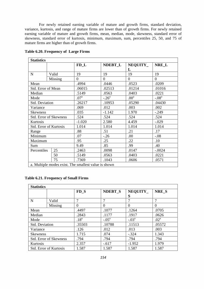
154
For newly retained earning variable of mature and growth firms, standard deviation,
variance, kurtosis, and range of mature firms are lower than of growth firms. For newly retained
earning variable of mature and growth firms, mean, median, mode, skewness, standard error of
skewness, standard error of kurtosis, minimum, maximum, sum, percentiles 25, 50, and 75 of
mature firms are higher than of growth firms.
Table 6.20. Frequency of Large Firms
Statistics
FD_L NDEBT_L NEQUITY_
L
NRE_L
N Valid 19 19 19 19
Missing 0 0 0 0
Mean .4994 .0446 .0523 .0209
Std. Error of Mean .06015 .02513 .01214 .01016
Median .5149 .0563 .0403 .0221
Mode .07a -.26
a .00
a -.08
a
Std. Deviation .26217 .10953 .05290 .04430
Variance .069 .012 .003 .002
Skewness .035 -1.142 1.970 -.249
Std. Error of Skewness .524 .524 .524 .524
Kurtosis -1.020 2.580 4.459 -.029
Std. Error of Kurtosis 1.014 1.014 1.014 1.014
Range .88 .51 .21 .17
Minimum .07 -.26 .00 -.08
Maximum .95 .25 .22 .10
Sum 9.49 .85 .99 .40
Percentiles 25 .2463 .0098 .0147 -.0024
50 .5149 .0563 .0403 .0221
75 .7369 .1043 .0606 .0571
a. Multiple modes exist. The smallest value is shown
Table 6.21. Frequency of Small Firms
Statistics
FD_S NDEBT_S NEQUITY_
S
NRE_S
N Valid 7 7 7 7
Missing 0 0 0 0
Mean .4497 .1077 .1264 .0705
Median .2843 .1177 .1917 .0626
Mode .18a -.05
a -.03
a .02
a
Std. Deviation .35503 .10788 .11513 .05572
Variance .126 .012 .013 .003
Skewness 1.715 .074 -.324 1.343
Std. Error of Skewness .794 .794 .794 .794
Kurtosis 2.357 -.617 -1.952 1.979
Std. Error of Kurtosis 1.587 1.587 1.587 1.587

155
Range .97 .31 .30 .16
Minimum .18 -.05 -.03 .02
Maximum 1.16 .27 .27 .18
Sum 3.15 .75 .89 .49
Percentiles 25 .2332 .0180 .0224 .0265
50 .2843 .1177 .1917 .0626
75 .6982 .2097 .2015 .0951
a. Multiple modes exist. The smallest value is shown
For financing deficit variable of large and small firms, mean, median, sum, percentiles
25, 50, and 75 of large firms are higher than of small firms. For financing deficit variable of large
and small firms, mode, standard deviation, variance, skewness, standard error of skewness,
kurtosis, standard error of kurtosis, range, minimum, and maximum of large firms are lower than
of small firms.
For net debt issue variable of large and small firms, variance of large firms is exactly the
same with small firms, while standard deviation, kurtosis, range, and sum of large firms are higher
than of small firms. For net debt issue variable of large and small firms, mean, median, mode,
skewness, standard error of skewness, standard error of kurtosis, minimum, maximum, and
percentiles 25, 50, and 75 of large firms are lower than of small firms.
For net equity issue variable of large and small firms, mode, skewness, kurtosis,
minimum, and sum of large firms are higher than of small firms. For net equity issue variable of
large and small firms, mean, median, standard deviation, variance, standard error of skewness,
standard error of kurtosis, range, maximum, percentiles 25, 50, and 75 of large firms are lower
than of small firms.
For newly retained earning variable of large and small firms, range of large firms are
higher than of small firms. For newly retained earning variable of large and small firms, mean,
median, mode, standards deviation, variance, skewness, standard error of skewness, kurtosis,
standard error of kurtosis, minimum, maximum. Sum, percentiles 25, 50, and 75 of large firms are
lower than of small firms.
Table 6.22. Frequency of Old Firms
Statistics
FD_O NDEBT_O NEQUITY_O NRE_O
N Valid 24 24 24 24
Missing 0 0 0 0
Mean .5014 .0635 .0686 .0271
Median .5032 .0638 .0412 .0244
Mode .07a -.26
a .00
a -.08
a
Std. Deviation .28980 .11226 .06884 .04352
Variance .084 .013 .005 .002
Skewness .447 -.842 1.244 -.316
Std. Error of
Skewness
.472 .472 .472 .472
Kurtosis -.550 2.194 .189 .046
Std. Error of .918 .918 .918 .918
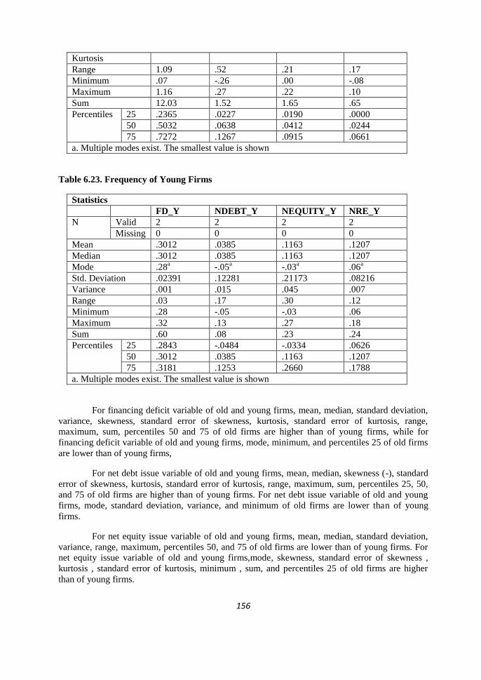
156
Kurtosis
Range 1.09 .52 .21 .17
Minimum .07 -.26 .00 -.08
Maximum 1.16 .27 .22 .10
Sum 12.03 1.52 1.65 .65
Percentiles 25 .2365 .0227 .0190 .0000
50 .5032 .0638 .0412 .0244
75 .7272 .1267 .0915 .0661
a. Multiple modes exist. The smallest value is shown
Table 6.23. Frequency of Young Firms
Statistics
FD_Y NDEBT_Y NEQUITY_Y NRE_Y
N Valid 2 2 2 2
Missing 0 0 0 0
Mean .3012 .0385 .1163 .1207
Median .3012 .0385 .1163 .1207
Mode .28a -.05
a -.03
a .06
a
Std. Deviation .02391 .12281 .21173 .08216
Variance .001 .015 .045 .007
Range .03 .17 .30 .12
Minimum .28 -.05 -.03 .06
Maximum .32 .13 .27 .18
Sum .60 .08 .23 .24
Percentiles 25 .2843 -.0484 -.0334 .0626
50 .3012 .0385 .1163 .1207
75 .3181 .1253 .2660 .1788
a. Multiple modes exist. The smallest value is shown
For financing deficit variable of old and young firms, mean, median, standard deviation,
variance, skewness, standard error of skewness, kurtosis, standard error of kurtosis, range,
maximum, sum, percentiles 50 and 75 of old firms are higher than of young firms, while for
financing deficit variable of old and young firms, mode, minimum, and percentiles 25 of old firms
are lower than of young firms,
For net debt issue variable of old and young firms, mean, median, skewness (-), standard
error of skewness, kurtosis, standard error of kurtosis, range, maximum, sum, percentiles 25, 50,
and 75 of old firms are higher than of young firms. For net debt issue variable of old and young
firms, mode, standard deviation, variance, and minimum of old firms are lower than of young
firms.
For net equity issue variable of old and young firms, mean, median, standard deviation,
variance, range, maximum, percentiles 50, and 75 of old firms are lower than of young firms. For
net equity issue variable of old and young firms,mode, skewness, standard error of skewness ,
kurtosis , standard error of kurtosis, minimum , sum, and percentiles 25 of old firms are higher
than of young firms.
157
For newly retained earning variable of old and young firms, mean, median, mode,
standard deviation, variance, minimum, maximum, percentiles 25,50, and 75 of old firms are
lower than of young firms. For newly retained earning variable of old and young firms, skewness,
standard error of skewness, kurtosis, standard error of kurtosis, range, and sum of old firms are
higher than of young firms.
6.5. Statistical Power Analysis of Hypotheses 1, 2, 3, and 4
To examine to what extent the theory is implied in our sample, we also analyse the
predictive power of the result. It consists of analysing the un-standardised beta coefficients, the
standardised beta coefficients, analysis of variance (ANOVA), coefficient of determination (R-
squared), and descriptive statistics.
A. The Un-standardised Beta Coefficients
B is the value for the regression equation for predicting the dependent variable from the
independent variable. These are called un-standardised coefficients because they are measured in
their natural units. As such, the coefficients cannot be compared with one another to determine
which one is more influential in the model, because they can be measured on different scales.
For hypothesis 1, (Constant) value of profitability, growth, tangibility, risk, and size on
short-term leverage as dependent variable is 0.138, B Coefficients of profitability, growth,
tangibility, risk, and size are -0.443, -0.230, 0.012, 1.218, and 0.092. (Constant) value of
profitability, growth, tangibility, risk, and size on long-term leverage as dependent variable is
0.141, B Coefficients of profitability, growth, tangibility, risk, and size are -0.296, 0.372, -0.004, -
0.712, and 0.138. (Constant) value of profitability, growth, tangibility, risk, and size on total
leverage as dependent variable is 0.207, B Coefficients of profitability, growth, tangibility, risk,
and size are -0.765, 0.104, 0.014, 0.506, and 0.229. (Constant) value of profitability, growth,
tangibility, risk, and size on market leverage as dependent variable is 1.283, B Coefficients of
profitability, growth, tangibility, risk, and size are -0.683, 0.106, -0.011, 0.142, and -0.375. From
these results, we can conclude that the highest value is market leverage while the lowest is long-
term leverage.
For hypothesis 2, each model for firms sample have only one predictor variable, then beta
is equivalent to the correlation coefficient between the predictor and the criterion variable. The
following is the result of (constant) value and beta coefficients of financing deficit on net debt
issued, net equity issued, and newly retained earning for all of sample of firms. (Constant) value of
financing deficit on net debt issued is 0.001, B coefficients of financing deficit is 0.281. It
indicates that if there is no financing deficit, then net debt issued is 0.001. If value of financing
deficit 1 is 1, then net debt issued is 0.282. (Constant) value of financing deficit on net equity
issued is -0.015, B coefficients of financing deficit is 0.169. It indicates that if there is no financing
deficit, then net equity issued is -0.015. If value of financing deficit is 1, then net equity issued is
0.154. (Constant) value of financing deficit on newly retained earning is 0.086, B coefficients of
financing deficit is -0.037. It indicates that if there is no financing deficit, then newly retained
earning is 0.086. If value of financing deficit is 1, then newly retained earning is 0.049. (Constant)
value of financing deficit on repurchase equity is -0.021, B coefficients of financing deficit is
0.000. It indicates that if there is no financing deficit, then repurchase equity is -0.021. If value of
financing deficit is 1, then repurchase equity is -0.021. From these results, we can conclude that
the highest value is net debt issue. It indicates that if firms face financing deficit, they tend to issue
more debt.
158
For hypothesis 3, (constant) value of net debt issued on the monthly and the yearly stock
price is positive. From the table in the appendix, we can conclude that the highest value is the
January stock price while the lowest value is the September stock price. (Constant) value of net
equity issued on monthly and yearly stock price is positive while net equity issued is negative.
(Constant) value of repurchase equity on monthly and yearly stock price is positive but not
significant.
For hypothesis 4, the result of (constant) value and beta coefficients of financing deficit
on net debt issued, net equity issued, and newly retained earning for growth and mature firms is as
follows. For growth firms, (constant) value of financing deficit on net debt issue is -0.106, beta
coefficients of financing deficit are 0.284. It indicates that if there is no financing deficit, then net
debt issue is -0.106, if value of financing deficit is 1, then net debt issue is 0.178. (Constant) value
of financing deficit on net equity issue is 0.021, beta coefficients of financing deficit is 0.073, it
indicates that if there is no financing deficit, then net equity issue is 0.021, if value of financing
deficit is 1, then net equity issue is 0.094. (Constant) value of financing deficit on newly retained
earning is 0.057, beta coefficients of financing deficit are -0.091. It indicates that if there is no
financing deficit, then newly retained earning is 0.057, if value of financing deficit is 1, then newly
retained earning is -0.034.
For mature firms, (constant) value of financing deficit on net debt issue is 0.026, beta
coefficients of financing deficit is 0.151. It indicates that if there is no financing deficit, then net
debt issue is 0.026. If value of financing deficit is 1, then net debt issue is 0.177. (Constant) value
of financing deficit on net equity issue is -0.005, B coefficients of financing deficit1 is 0.058. It
indicates that if there is no financing deficit, then net equity issue is -0.005. If value of financing
deficit is 1, then net equity issue is 0.053. (Constant) value of financing deficit on newly retained
earning is 0.074, beta coefficients of financing deficit are -0.042. It indicates that if there is no
financing deficit, then newly retained earning is 0.074. If value of financing deficit is 1, then
newly retained earning is 0.032.
B. The Standardised Beta Coefficients
Beta(s) are the standardised coefficients. These are the coefficients that we would obtain
if we standardised all of the variables in the regression, including the dependent and all of the
independent variables, and ran the regression. By standardising the variables before running the
regression, we have put all of the variables on the same scale, and we can compare the magnitude
of the coefficients to see which one has more of an effect. We will also notice that the larger betas
are associated with the larger t-values. The standardised beta coefficients give a measure of the
contribution of each variable to the model. A large value indicates that a unit change in this
predictor variable has a large effect on the criterion variable.
For hypothesis 1, standardised beta coefficients of profitability, growth, tangibility, risk,
and size on short-term leverage, long-term leverage, total leverage, market leverage are as follow:
standardised coefficients of profitability, growth, tangibility, risk, and size on short-term leverage
as dependent variable are -0.277, -0.196, 0.071, 0.346, and 0.136. Standardised coefficients of
profitability, growth, tangibility, risk, and size on long-term leverage as dependent variable are -
0.213, 0.364, -0.029, -0.232, and 0.234. Standardised coefficients of profitability, growth,
tangibility, risk, and size on total leverage as dependent variable are -0.502, 0.093, 0.090, 0.151,
and 0.356. Standardised coefficients of profitability, growth, tangibility, risk, and size on market
leverage as dependent variable are as follow: -0.513, 0.109, -0.080, 0.049, and -0.666.

159
For hypothesis 2, the result of the standardised beta coefficients of financing deficit on
net debt issued, net equity issued, and newly retained earning for all samples of firms is explained
as follows. Standardised coefficients of financing deficit (the predictor) on net debt issued the
(criterion) is 0.775. Standardised coefficients of financing deficit (the predictor) on net equity
issued the (criterion) is 0.464. Standardised coefficients of financing deficit (the predictor) on
newly retained earning the (criterion) is -0.236. Standardised coefficients of financing deficit (the
predictor) on repurchase equity (criterion) is -0.002.
It is the same with the result of unstandardised beta coefficients, standardised coefficients
of financing deficit on net debt issued is the highest. In other words the correlation coefficient
between financing deficit on net debt issued is the strongest. It indicates that if firms face 1%
financing deficit then they tend to issue 28.1% net debt and/or 16.9% net equity.
For hypothesis 3, standardised coefficients of net debt issued on monthly and yearly stock
price are positive, ranging from 0.189 to 0.159. From these results, we can conclude that the
highest value is the January stock price while the lowest value is the December stock price.
Standardised coefficients of net equity issued on monthly and yearly stock price are
positive, ranging from -0.082 to -0.064. From these results, we can conclude that the highest value
is the September stock price while the lowest value is the December stock price.
Standardised coefficients of repurchase equity on monthly and yearly stock price are
positive, ranging from 0.881 to 0.347. From these results, we can conclude that the highest value is
the November stock price while the lowest value is the February stock price.
For hypothesis 4, the result of the standardised beta coefficients of financing deficit on
net debt issued, net equity issued, and newly retained earning for growth and mature firms is
explained as follows.
For mature firms, standardised coefficients of financing deficit 1 on its net debt issue is
0.383, it means that the correlation coefficient between the predictor and the criterion variable is
0.383. Standardised coefficient of financing deficit on its net equity issue is 0.254. It means that
the correlation coefficient between the predictor and the criterion variable is 0.254. Standardised
coefficient of financing deficit on its newly retained earning is -0.177. It means that the correlation
coefficient between the predictor and the criterion variable is -0.177.
For growth firms, standardised coefficients of financing deficit 1 on net debt issue is
0.385, it means that the correlation coefficient between the predictor and the criterion variable is
0.385. It is higher than mature firms. Standardised coefficient of financing deficit on net equity
issue is 0.177. It means that the correlation coefficient between the predictor and the criterion
variable is 0.177. It is lower than mature firms. Standardised coefficient of financing deficit of
growth firms on its newly retained earning is -0.285. It means that the correlation coefficient
between the predictor and the criterion variable is -0.285. It is more negative than mature firms.
C. Analysis of Variance (ANOVA)
The F-statistic will be calculated for analysis of variance (ANOVA) to test whether group
population means are all equal or not. When the F-statistic is found significant, we may conclude
that at least one of the population means of the groups differs from the others but ANOVA does
not tell us which groups are different from which others (Bekiro, 2001).

160
For hypothesis 1, short-term leverage, long-term leverage, total leverage, market leverage
as dependent variable and growth, tangibility, risk, size, and profitability as predictors, reaches
statistical significance with F-value of 18.878 and significant value of 0.000 for short-term
leverage, F-value of 15.362 and significant value of 0.000 for long-term leverage, F value of
72.059 and significant value of 0.000 for total leverage, F-value of 67.082 and significant value of
0.000 market leverage. Hence, the statistical significance as depicted in the ANOVA analysis (see
table in appendix) indicates that the models of hypothesis 1 reach statistical significance less than
5%.
For hypothesis 2, after reaching F-statistic result analysis of variance to test whether
group population means are all equal or not, we did not find significant result for all models.
F-value between net debt issued and financing deficit is 76.620 with significance value of
.000. F-value between net equity issued and financing deficit is 13.971 with significance value of
.000. F-value between newly retained earning and financing deficit is 3.010 with significance
value of .089. F-value between repurchase equity and financing deficit is 0.000 with significance
value of 0.993. F-value between net debt issued and financing deficit is higher than F-value
between net equity issued and financing deficit.
From these results, the significance F-values obtained were between financing deficit and
net debt issued and net equity issued, while F-values between financing deficit and newly retained
earning and repurchase equity were not significant.
For hypothesis 3, the statistical significance as depicted in the table of ANOVA shows
that variable of issued debt from January to December did not yield statistical significance The
statistical significance from January to December and yearly stock price became weaker.
For hypothesis 4, for mature and growth firms, the statistical significance as shown in the
ANOVA table in appendix indicates that the models for growth and mature firms reach statistical
significance of less than 5%.
For mature firms, F-value between net debt issue and financing deficit is 15.463 with
significance value of 0.000. F-value between net equity issue and financing deficit is 6.196 with
significance value of 0.015.
For growth firms, F-value between net debt issue and financing deficit is 22.556 (it is
higher than mature firm) with significance value of 0.000. F-value between net equity issue and
financing deficit is 4.219 (it is lower than mature firm) with significance value of 0.042.
D. Coefficient of Determination (R-squared)
For hypotheses 1, R Squared (R2) is the square of the measure of correlation and indicates
the proportion of the variance in the criterion variable which is accounted for by our model. For
hypotheses 1, we also see the adjusted R-square which attempts to yield a more honest value to
estimate the R-squared for the population. When the number of observations is small and the
number of predictors is large, there will be a much greater difference between R-square and
adjusted R-square. By contrast, when the number of observations is very large compared to the
number of predictors, the value of R-square and adjusted R-square will be much closer.
R-squared for hypothesis 1 would be the value between short-term leverage, long-term
leverage, total leverage, market leverage as dependent variable and growth, tangibility, risk, size,
and profitability as predictors.
161
R-squared shows a predictor profitability, growth, tangibility, risk, and size of 0.332 with
short-term leverage as dependent variable. This means that 33.2% of the short-term leverage could
be explained by the existence of those variables. The adjusted R-squared value of tangibility,
growth, risk, size, and profitability as predictors for short-term leverage is 0.314. These provide
evidence that 31.4% of the short-term leverage could be explained by the existence of these
predictors.
R-squared shows a predictor profitability, growth, tangibility, risk, and size of 0.288 with
long-term leverage as dependent variable. This means that 28.8% of the long-term leverage could
be explained by the existence of those variables. The adjusted R-squared value of tangibility,
growth, risk, size, and profitability as predictors for long-term leverage is 0.269. These provide
evidence that 26.9% of the long-term leverage could be explained by the existence of these
predictors.
R-squared shows a predictor profitability, growth, tangibility, risk, and size of 0.655 with
total leverage as dependent variable. This means that 65.5% of the total leverage could be
explained by the existence of those variables. The adjusted R-squared value of tangibility, growth,
risk, size, and profitability as predictors for total leverage is 0.646. These provide evidence that
64.6% of the total leverage could be explained by the existence of these predictors.
R-squared shows a predictor of profitability, growth, tangibility, risk, and size of 0.638
with market leverage as dependent variable. This means that 63.8% of the market leverage could
be explained by the existence of those variables. The adjusted R-squared value of tangibility,
growth, risk, size, and profitability as predictors for market leverage is 0.629. These provide
evidence that 62.9% of the market leverage could be explained by the existence of these
predictors. Overall, there is no multicollinearity in the regression model of hypothesis 1.
For hypothesis 2, R-squared would be the value between the financing deficit and net
debt and net equity issue as dependent variables. For all sample of firms, R-squared shows a
predictor financing deficit of 0.600, 0.215, 0.056 with net debt issue, net equity issue, newly
retained earning as dependent variables. This means that 60%, 21.5%, and 5.6% of the net debt
issue, net equity issue, and newly retained earning could be explained by the existence of
financing deficit.
For all firms, R-squared shows a predictor financing deficit of 0.000 with repurchase
equity as dependent variables. This means that the repurchase equity almost cannot be explained
by the existence of financing deficit.
For augmented models, for all firms, adjusted R-squared shows a predictor financing
deficit and financing deficit 1 square of (0.603) and with net debt issue as dependent variable. This
means that 60.3% of the net debt issue can be explained by the existence of financing deficit and
financing deficit square.
R-squared of a predictor financing deficit with net debt issue as dependent variable is
higher than net equity issue. This means that the percentage of the net debt issue can be explained
more than net equity issue by the existence of financing deficit.
For hypothesis 3, R-squared would be the correlation between the stock price and the net
debt as dependent variables, the net equity and the debt issuance to repurchase equity as
independent variable.
162
R-squared shows a predictor net debt issued between 0.025 to 0.036 and 0.001 with
monthly and yearly stock price as dependent variables. This means that 2.5% to 3.6%, and 0.1% of
the monthly and yearly stock price could be explained by the existence of net debt issued. We can
see that a predictor net debt issued on January stock price as dependent variables has the highest
R-squared, while R-squared December stock price was the lowest.
The R-squared of a predictor of net equity issuance on January to December ranged
between 0.007 to 0.004 and the yearly stock price of 0.004 as dependent variable. This means that
between 0.7 - 0.4% and 0.4% of the increasing or decreasing of stock price could be explained by
the existence of net equity issue. On September the R-squared got the highest figure, while in
February, March, May, June, and December, it reached the lowest figure.
For all firms, from January to December and yearly stock price, R-squared showed a
predictor issue debt to repurchase equity of between 0.314-0.162 and 0.130 with the stock price as
dependent variable. This means that between 31.4-16.2% and 13.0% of the increasing or
decreasing of stock price could be explained by the existence of issue debt to repurchase equity.
For all firms, R-squared shows a predictor issue debt to repurchase equity on the
December stock price as dependent variables, has the highest R-squared, while R-squared of the
February stock price has the lowest.
For hypothesis 4, R-squared consists of the value for growth and mature firms. For
mature firms, R-squared shows a predictor financing deficit of 0.147 and 0.064 with net debt issue
and net equity issue as dependent variable. This means that 14.7% and 6.4% of the net debt issue
and net equity issue could be explained by the existence of financing deficit.
For growth firms, R-squared shows a predictor financing deficit of 0.148 (it is higher than
of mature firms) and 0.031 (it is lower than of mature firms) with net debt issue and net equity
issue as dependent variable. This means that 14.8% and 3.1% of the net debt issue and net equity
issue could be explained by the existence of financing deficit. Therefore there is no
multicollinearity in the regression model.
For augmented models of mature firms, adjusted R-squared shows a predictor of
financing deficit and financing deficit square of 0.229 and with net debt issue as dependent
variable. This means that 14.8% of the net debt issue could be explained by the existence of
financing deficit and financing deficit square.
For growth firms, adjusted R-squared shows a predictor financing deficit and financing
deficit square of 0.273 (it is higher than mature firm) and with net debt issue as dependent
variable. This means that 14.8% of the net debt issue could be explained by the existence of
financing deficit and financing deficit square.
E. Descriptive Statistics
For hypothesis 1, the average value of short-term leverage is 0.3665 while long-term
leverage is 0.2704, total leverage is 0.6461 and market leverage is 0.7890. The average value of
tangibility, growth, risk, size, and profitability are 0.0717, 0.3887, 15.0107, 0.0747, and 0.8810.
From these results, the highest average is market leverage.
For hypotheses 2, the average value of each variable of hypothesis 2 for all samples of
firms is as follows: The average value of net debt issued is 0.1555 while net equity issued is
0.0777, and newly retained earning is 0.0656. The average value of financing deficit on net debt
163
issued, net equity issued, and newly retained earning is 0.5493. The average value of net debt
issued is higher than net equity issued, hence if firms face financing deficit, they rely more heavily
on debt than on equity (indicated by R2, anova, and coefficient of regression). When firms issue
debt to repurchase equity, the average of net debt issued to repurchase equity is 0.149302, while
the average of repurchase equity is negative 0.021233. The financing deficit they face is 0.691921.
From this result we concluded that the average value of net debt issued is the highest.
For variables of hypothesis 3, the monthly stock price is in the range of 2558.6813 to
2384.4211 with July as the highest while the lowest is October. Meanwhile, the yearly stock price
is 3622.2704. The average value of net equity is 0.0317 to 0.0363, while the average value of
repurchase equity is -0.020687.
For hypothesis 4, descriptive statistics for variables of hypothesis 4 consist of average
value of growth and mature firms. Net debt issue (0.0484) of growth firms (NDebt_G) is lower
than net debt (0.0800) of mature firms (NDebt_M), while net equity issue 0.0610 of growth
(NEquity_G) firms is higher than net equity issue 0.0156 of mature firms (NEquity_M) as growth
firm has lower cashflow. The average value of financing deficit for the growth firms is 0.5520
while that of the mature firms is 0.3682 as mature firms has higher cashflow than growth firm.
Even though growth firms issue more equity than mature firms, and mature firms issue
more debt than growth firms, but when mature firms face financing deficit, they rely more heavily
on equity while growth firms rely more heavily on debt. It indicated by R2, anova, coefficient of
regression and augmented. A mature firm has higher cash flow than a growth firm to secure the
debt.
Financing deficit of growth firms is higher than financing deficit of mature firms, as
growing firms have lower cashflow than mature firms. Dividend (0.0026) of growing firms is
lower than dividend (0.0554) of mature firms. Mature firms pay more dividend to shareholders as
they have more cash flow to distribute to shareholders. Long-term leverage 0.3136 of growth firms
is higher than long-term leverage (0.2029) of mature firms. Fixed asset (0.4664) of growth firms is
higher than fixed asset (0.2815) of mature firms. dWorking capital (0.0637) of growth firms is
lower than dWorking capital (0.1016) of mature firms. Cashflow (0.0277) of growth firms is lower
than cashflow (0.0997) of mature firms. Newly retained earning (0.0075) of growth firms is lower
than newly retained earning (0.0587) of mature firms.
6.6. Regression Assumptions of Hypotheses 1, 2, 3, and 4
Before analysing regression coefficients of variables, we must first make several
assumptions about the population of the research. They represent an idealisation of reality, and as
such, they are never likely to be entirely satisfied for the population in any real study (Van Horne,
1998). A good regression model should not have the following assumptions:
1. Multicollinearity
The goal of the multicollinearity test of hypotheses 1, 2, 3, and 4 is to analyse whether there is
correlation between variables. In our research, we test multicollinearity in the regression model by
testing the correlation matrix (Ghozali, 2002), the tolerance values and VIF (Hair et al. 1998). Our
results are as follow:
164
Correlations between Variables
For hypothesis 1, the table gives details of the correlation between each pair of variables.
We do not want strong correlations between the criterion and the predictor variables. The values
here are acceptable.
From the correlations matrix, it shows that there is no quite high correlation value (more
than 0.90). Correlation coefficient between profitability and tangibility is -0.394 with significant
value of 0.000. This is an indication that the higher/lower profitability the lower/higher tangibility.
Correlation coefficient between profitability and size is -0.192 with significant value of 0.004.
This is an indication that the higher/lower profitability the lower/higher size of the firm.
Correlation coefficient between profitability and risk is -0.421 with significant value of 0.000. This
is an indication that the higher/lower profitability the lower/higher risk. Correlation coefficient
between profitability and growth is -0.210 with significant value of 0.002. This is an indication
that the higher/lower profitability the lower/higher growth. Correlation coefficient between size
and tangibility is 0.448 with significant value of 0.000. This is an indication that the higher/lower
size, the higher/lower tangibility. Correlation coefficient between size and growth is 0.243 with
significant value of 0.000. This is an indication that the higher/lower size the higher/lower growth.
Correlation coefficient between risk and growth is 0.222 with significant value of 0.001. This is an
indication that the higher/lower risk the higher/lower growth. From this result we concluded that
multicollinearity does not exist in the regression model of hypothesis 1.
For hypothesis 2, correlation between net debt and net equity issued and financing deficit
are significantly positive, while correlation between newly retained earning and financing deficit
are insignificantly negative. For firms, correlation between repurchase equity and financing deficit
are insignificantly negative.
For hypothesis 3, correlation between net debt and January-June stock price are
significantly positive while correlation between net debt and July-December stock price are
positive but not significant. Correlation between net equity and the yearly stock price or the price
for each month during the year is negative but not significant. But if we compare with the
repurchase equity, the stock price is positive but not significant.
For hypothesis 4, the values here are acceptable. For mature and growing firms,
correlation between net debt and net equity issue and financing deficit are positively significant. It
indicates that the higher financing deficit the bigger the net debt and net equity issue.
The Tolerance and Variance Inflation Factor (VIF) Value
For hypothesis 1, the objective of analysing the tolerance values are to measure the
correlation between the predictor variables which can vary between 0 and 1. The closer to zero the
tolerance value is for a variable, the stronger the relationship between this and the other predictor
variables. We should worry about variables that have a very low tolerance. SPSS will not include a
predictor variable in a model if it has a tolerance of less that 0.0001. Meanwhile, variance inflation
factor (VIF) value is an alternative measure of collinearity (in fact it is the reciprocal of tolerance)
in which a large value indicates a strong relationship between predictor variables.
For variables of hypothesis 1, short-term leverage, long-term leverage, total leverage, and
market leverage as dependent variables and growth, tangibility, risk, size, and profitability as
predictors, the tolerance values were also above the cut-off point 0.10 and the VIF values were
below 10, indicating that multicollinearity was not a problem (Hair et al. 1998).
165
For variables of hypothesis 2, the tolerance values for net debt issued, net equity issued,
newly retained earning, repurchase equity, financing deficit1 were above the cut-off point 0.10 and
the VIF values were below 10.
For variables of hypothesis 3, the tolerance values for net debt issued on monthly and
yearly stock price were above the cut-off point 0.10 and the VIF values were below 10. While the
tolerance values for net equity issued on monthly and yearly stock price were above the cut-off
point 0.10, the VIF values were below 10. The tolerance values for issuing debt to repurchase
equity on monthly and yearly stock price were above the cut-off point 0.10 and the VIF values
were below 10.
For variables of hypothesis 4, for mature and growing firms, the tolerance values for net
equity issued, net debt issued, and financing deficit 1 were above the cut-off point 0.10 and the
VIF values were below 10. Hence, from tolerance and VIF values of hypotheses 1, 2, 3, and 4
testing results indicate that multicollinearity was not a problem.
2. Autocorrelation
For hypotheses 1, 2, 3, and 4, a test of autocorrelation aims to examine whether in a linear
regression model has correlation between gadfly errors in the period t with an error in the periodt-1
(before). One of the methods that we used to detect autocorrelation is the Durbin Watson (DW).
DW value shows that there is no autocorrelation in the regression model.
As a conservative rule of thumb, Field (2009) suggests that DW values less than 1 or
greater than 3 are definitely cause for concern, however, values closer to 2 may still be
problematic depending on the sample and model.
For hypothesis 1, DW value between short-term leverage as dependent variable and
predictors of growth, tangibility, risk, size, and profitability is 1.335. For all firms, DW value
between long-term leverage as dependent variable and predictors of growth, tangibility, risk, size,
and profitability is 1.274. For all firms, DW value between total leverage as dependent variable
and predictors of growth, tangibility, risk, size, and profitability is 0.994. For all firms, DW value
between market leverage as dependent variable and predictors of growth, tangibility, risk, size, and
profitability is 1.133. A value greater than 2 indicates a negative correlation between adjacent
residuals whereas a value below 2 indicates a positive correlation.
For hypothesis 2, DW value between net debt issued, net equity issued, newly retained
earning, repurchase equity were 1.667, 2.502, 1.494, and 1.907. A value greater than 2 indicates a
negative correlation between adjacent residuals whereas a value below 2 indicates a positive
correlation.
For hypothesis 3, DW value of predictor net debt issued and monthly stock price as
dependent variables ranged from 0.862 to 0.546. DW value of predictor net debt issued and yearly
stock price as dependent variable was 1.558. A value greater than 2 indicated a negative
correlation between adjacent residuals whereas a value below 2 indicated a positive correlation.
For net equity issued, it ranged from 0.820 to 0.532. The DW value of predictor was 1.574. The
DW value of predictor for debt issuance to repurchase equity ranged from 1.049 to 0.598. The DW
value for yearly stock price as dependent variable was 1.577.
For hypothesis 4, DW value of net debt and net equity issue and financing deficit are
1.602 and 2.284. For growing firms, DW value between net debt and net equity issue and
financing deficit are 1.670 and 2.108. A value greater than 2 indicates a negative correlation

166
between adjacent residuals whereas a value below 2 indicates a positive correlation. Hence, for
growing and mature firms, there are no DW values less than 1 or greater than 3 which definitely
cause concern.
3. Heteroscedasticity
Test of heteroscedasticity of hypotheses 1, 2, 3, and 4 aims to interpret whether the
regression model has the differences residual variance from one observation to another observation
(Ghozali, 2002). If the residual variance from one observation to another observation is the same,
it is called homoscedasticity.
The graphic of scatterplot (in appendix) shows that the dots have not established a
specific pattern. Some of the dots located adjacent but some other dots spread above and below the
numbers of 0 at the axis Y. Thus, data in the graphics exhibits homoscedasticity.
4. Normally Distributed
From the result of testing hypotheses 1, 2, 3, and 4, to test the normal distribution that we
can see from the graphics of histogram and normal P-P plot (in appendix), we concluded that the
histogram gave the normal pattern of distribution. Meanwhile, the graphic of normal P-P plot
shows that the dots spread around the diagonal line, and the spreading follows the diagonal line.
Both of graphics show that the data meets reasonable assumption of normality.
Therefore, based on the results of assumptions of population described above, the
regression model does not have the assumptions of heteroscedasticity, multicollinearity,
autocorrelation, and the data are normally distributed. Thus, our regression model is appropriate to
use for testing the hypotheses 1, 2, 3, and 4.
6.7. Results of Panel Data Regression Analysis and the Comparison to Regression Analysis
We applied mixed-effect linear regression to analyse longitudinal/panel data which
reported both fixed effects and random effects. Panel data (also known as longitudinal or cross-
sectional time-series data) is a dataset in which the behaviour of entities is observed across time.
Panel data allows us to control for variables we cannot observe or measure; or variables that
change over time but not across entities with panel data we can include variables at different levels
of analysis suitable for multilevel or hierarchical modeling.
Two techniques use to analyse panel data are fixed effects and random effects. Hence, we
use multilevel mixed-effect models to analyse our data with using mixed-effect linear regression
so that we can report both fixed effects and random effects of the models. Fixed-effects are used
whenever we are only interested in analysing the impact of variables that vary over time. Fixed-
effects explore the relationship between predictor and outcome variables within an entity. Each
entity has its own individual characteristics that may or may not influence the predictor variables.
When using fixed-effects, we assume that something within the individual may impact or bias the
predictor or outcome variables and we need to control for this. This is the rationale behind the
assumption of the correlation between the entity‟s error term and predictor variables. Fixed-effects
remove the effect of those time-invariant characteristics from the predictor variables so we can
assess the predictors‟ net effect.
Another important assumption of the fixed-effects model is that those time-invariant
characteristics are unique to the individual and should not be correlated with other individual
characteristics. Each entity is different, therefore the entity‟s error term and the constant (which
captures individual characteristics) should not be correlated with the others. If the error terms are

167
correlated then fixed-effects is not suitable since inferences may not be correct and we need to
model that relationship (probably using random-effects).
Meanwhile, the rationale behind the random effects model is that, unlike the fixed effects
model, the variation across entities is assumed to be random and uncorrelated with the predictor or
independent variables included in the model: “…the crucial distinction between fixed and random
effects is whether the unobserved individual effect embodies elements that are correlated with the
regressors in the model, not whether these effects are stochastic or not” (Green, 2008).
If we have reason to believe that differences across entities have some influence on our
dependent variable then we should use random effects. An advantage of random effects is that we
can include time invariant variables. Random effects assume that the entity‟s error term is not
correlated with the predictors which allows for time-invariant variables to play a role as
explanatory variables. In random-effects we need to specify those individual characteristics that
may or may not influence the predictor variables. The problem with this is that some variables
may not be available therefore leading to omitted variable bias in the model. Random-effects are
allowed to generalise the inferences beyond the sample used in the model.
Tables in appendix are our results of mixed-effect linear regression which reports both
fixed effects and random effects for each hypothesis. Meanwhile, if we compare the results of
regression and panel data regression, the following are the summary for each hypothesis and
analysis.
Table 6.24. Summary of Panel Data Regression and Regression Results of Hypothesis 1
Variables Panel Data Regression Result Regression Result
PRFT Negative significant Negative significant
TANG Negative significant Negative significant
SIZE Positive not significant Positive not significant
RISK Positive significant Positive significant
GROW Positive significant Positive significant
Dependent variable: STL
Variables Panel Data Regression Result Regression Result
PRFT Negative significant Negative significant
TANG Positive significant Positive significant
SIZE Negative not significant Negative not significant
RISK Negative not significant Negative significant
GROW Positive significant Positive significant
Dependent variable: LTL
Variables Panel Data Regression Result Regression Result
PRFT Negative significant Negative significant
TANG Positive significant Positive not significant
SIZE Positive not significant Positive not significant
RISK Positive not significant Positive significant
GROW Positive significant Positive significant
Dependent variable: TLV
Variables Panel Data Regression Result Regression Result
PRFT Negative significant Negative significant
TANG Positive significant Positive significant
SIZE Positive not significant Negative not significant
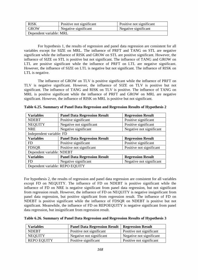
168
RISK Positive not significant Positive not significant
GROW Negative significant Negative significant
Dependent variable: MRL
For hypothesis 1, the results of regression and panel data regression are consistent for all
variables except for SIZE on MRL. The influence of PRFT and TANG on STL are negative
significant while the influence of RISK and GROW on STL are positive significant. However, the
influence of SIZE on STL is positive but not significant. The influence of TANG and GROW on
LTL are positive significant while the influence of PRFT on LTL are negative significant.
However, the influence of SIZE on LTL is negative but not significant. The influence of RISK on
LTL is negative.
The influence of GROW on TLV is positive significant while the influence of PRFT on
TLV is negative significant. However, the influence of SIZE on TLV is positive but not
significant. The influence of TANG and RISK on TLV is positive. The influence of TANG on
MRL is positive significant while the influence of PRFT and GROW on MRL are negative
significant. However, the influence of RISK on MRL is positive but not significant.
Table 6.25. Summary of Panel Data Regression and Regression Results of Hypothesis 2
Variables Panel Data Regression Result Regression Result
NDEBT Positive significant Positive significant
NEQUITY Negative not significant Positive significant
NRE Negative significant Negative not significant
Independent variable: FD
Variables Panel Data Regression Result Regression Result
FD Positive significant Positive significant
FDSQR Positive not significant Positive not significant
Dependent variable: NDEBT
Variables Panel Data Regression Result Regression Result
FD Negative significant Negative not significant
Dependent variable: REPO EQUITY
For hypothesis 2, the results of regression and panel data regression are consistent for all variables
except FD on NEQUITY. The influence of FD on NDEBT is positive significant while the
influence of FD on NRE is negative significant from panel data regression, but not significant
from regression result. However, the influence of FD on NEQUITY is negative insignificant from
panel data regression, but positive significant from regression result. The influence of FD on
NDEBT is positive significant while the influence of FDSQR on NDEBT is positive but not
significant. Meanwhile, the influence of FD on REPOEQUITY is negative significant from panel
data regression, but insignificant from regression result.
Table 6.26. Summary of Panel Data Regression and Regression Results of Hypothesis 3
Variables Panel Data Regression Result Regression Result
NDEBT Positive not significant Positive not significant
NEQUITY Negative not significant Negative not significant
REPO EQUITY Positive significant Positive not significant

169
Dependent Variable: P_Yearly
For hypothesis 3, the results of regression and panel data regression are consistent for all
variables. The influence of NDEBT on P_Yearly is positive insignificant while the influence of
NEQUITY on P_Yearly is negative insignificant. Meanwhile, the influence of REPOEQUITY on
P_Yearly is positive significant from panel data regression, but positive insignificant from
regression result.
Table 6.27. Summary of Panel Data Regression and Regression Results of Hypothesis 4
Variables Panel Data Regression Result Regression Result
NDEBT_M Positive significant Positive significant
NEQUITY_M Positive significant Positive significant
NRE_M Negative significant Negative not significant
Independent Variable: FD_M
Variables Panel Data Regression Result Regression Result
FD_M Positive significant Positive significant
FDSQR_M Negative not significant Negative significant
Dependent Variable: NDEBT_M
Variables Panel Data Regression Result Regression Result
NDEBT_G Positive significant Positive significant
NEQUITY_G Positive significant Positive significant
NRE_G Negative significant Negative significant
Independent Variable: FD_G
Variables Panel Data Regression Result Regression Result
FD_G Positive significant Positive significant
FDSQR_G Negative significant Negative significant
Dependent Variable: NDEBT_G
For hypothesis 4, for mature firms, the results of regression and panel data regression are
consistent for all variables. The influence of FD on NDEBT and NEQUITY are positive
significant while the influence of FD on NRE is negative significant from panel data regression,
but not significant from regression result. The influence of FD on NDEBT is positive significant
while the influence of FDSQR on NDEBT is negative significant from regression result, but not
significant from panel data regression result.
For hypothesis 4, for growth firms, the results of regression and panel data regression are
consistent for all variables. The influence of FD on NDEBT and NEQUITY are positive
significant while the influence of FD on NRE is negative significant. The influence of FD on
NDEBT is positive significant while the influence of FDSQR on NDEBT is negative significant.
170
7. CONCLUSION
7.1. Conclusion
Based on the results analysis of each hypotheses testing, overall, our conclusions are as
follow: For hypothesis 1, profitability has a negative significant regression coefficient on short-
term leverage, long-term leverage, and total leverage. This suggests that highly profitability firms
are less likely to use short-term leverage, long-term leverage, and total leverage, for financing their
investments than the low profitability firms. Finally, profitability has a negative significant
regression coefficient on market leverage. This suggests that highly profitability firms are less
likely to use market leverage for financing their investments than the low profitability firms.
Tangibility has a negative significant regression coefficient on short-term leverage, this
suggests that highly tangibility firms are less likely to use short-term leverage for financing their
investments than the low tangibility firms. Tangibility has a positive significant regression
coefficient on long-term leverage; this suggests that highly tangibility firms are more likely to use
long-term leverage for financing their investments than the low tangibility firms.
Tangibility has a positive but not significant regression coefficient on total leverage,
while tangibility has a positive significant regression coefficient on market leverage. This suggests
that highly tangibility firms are more likely to use market leverage for financing their investments
than the low tangibility firms.
Size has a positive but not significant regression coefficient on short-term leverage and
total leverage, while size has a negative but not significant regression coefficient on long-term
leverage. However, size has a negative significant regression coefficient on market leverage. This
suggests that high size firms are less likely to use market leverage for financing their investments
than low size firms.
Risk has a positive significant regression coefficient on short-term leverage and total
leverage. This suggests that highly risk firms are more likely to use short-term leverage and total
leverage for financing their investments than the low risk firms. Meanwhile, risk has a negative
significant regression coefficient on long-term leverage this suggests that highly risk firms are less
likely to use long-term leverage for financing their investments than the low risk firms. However,
risk has a positive but not significant regression coefficient on market leverage.
Growth has a positive significant regression coefficient on short-term, long-term, and
total leverage, which suggests that highly growth firms are more likely to use short-term, long-
term, and total leverage for financing their investments than the low growth firms. However,
growth has a negative significant regression coefficient on market leverage. This suggests that
high growth firms are less likely to use market leverage for financing their investments than the
low growth firms.
For hypothesis 2, from tables, we can conclude that the financing deficit has positive
significant effects on net debt issue and on net equity issue. This result suggests that high deficit
firms would tend to issue more net debt and net equity to finance the financing deficit. The
financing deficit has negative but not significant effects on newly retained earning. This result
suggests that high deficit firms would not tend to use newly retained earning to finance the
financing deficit. The financing deficit has negative but not significant effects on repurchase
171
equity. This result suggests that high deficit firms would not tend to repurchase equity to finance
the financing deficit.
From the descriptive table, we see that the amount of net debt issue is more than net
equity issue and it is consistent with regression results. For the augmented model, our result shows
a positive coefficient on the financial deficit and also on the squared deficit term. However, for the
squared deficit term, the coefficient was not significant. It implies that firms are limited by their
debt capacity constraints and they have to resort to issuing equity. A squared deficit coefficient
that is not large in absolute value implies a less reliance on equity finance for values of the
financing deficit.
Therefore, we can conclude that our sample of firm prefers external to internal financing
and debt to equity if external financing is used. However, firms are limited by their debt capacity
constraints and they have to resort to issuing equity.
For hypothesis 3, the results indicate that net debt has no positive significant impact on
the stock price of from January to December. This indicates that net debt has no significant impact
on the yearly stock price. Net equity has no negative significant impact on the stock price from
January to December. The result indicates that net equity has no significant impact on the stock
price. This result suggests that firms that issue more net equity would tend to have decreasing
stock price, while issue more net debt, the firm would tend to have increasing stock price. Result
also suggests that firms that repurchase equity would tend to have increasing stock price.
For hypothesis 4, the growing firms, from tables we can conclude that the financing
deficit has positive significant effects on net debt issue, financing deficit has positive significant
effects on net equity issue, and financing deficit has negative significant effects on newly retained
earning. For mature firms, from tables we can conclude that the financing deficit has positive
significant effects on net debt issue and net equity issue, while financing deficit has negative
insignificant effects on newly retained earning. From these results, we can conclude that our
mature and the sample of growth firms prefer external to internal financing and debt to equity if
external financing is used. Overall, we find that the pecking order theory describes the financing
patterns of growth firms better than mature firms as mature firms are more closely adopted by
analysts and are better known to investors, and hence, should suffer less from problems of
information asymmetry.
7.2 Conclusion regarding Result and Its Consistency with Condition of Indonesian Capital
Market
Our findings are implied that high growth firms in the manufacturing sector of the LQ45 Index are
more likely to use short-term leverage, long-term leverage, and total leverage for financing their
investments than low growth firms. However, firms with relatively high growth use less market
leverage. Firms with relatively high growth will tend to issue securities less subject to information
asymmetries, i.e. shot-term debt. Firms in the manufacturing sector of the LQ45 Index with
relatively high growth are also to use more long-term and total leverage as when they use long-
term leverage and total leverage for financing their investments, they have asset tangibility to
secure their long-term debt.
Even though high growth firms will face more information asymmetries, in the Indonesia
Capital Market has already had the regulation to minimise information asymmetries, such as
Regulation of Bapepam-LK No.X.K.1 regarding disclosure of information that must be announced
to the public, and the attachment of Chairman Decision of Bapepam No.Kep-86/PM/1996 dated 24
January 1996 and Decision of the Board of Directors of PT. Indonesia Stock Exchange No: Kep-
172
306/BEJ/07-2004 dated July 19, 2004 concerning Rule Number I-E on the Obligation to Deliver
Information.
For firms in the manufacturing sector of the LQ45 Index, financing constraints will be
more easily solved, as they have more access to banking. Banks will be more recognised and
trusted than the companies. It is not excessive considering each moment banks can determine the
condition of the company's financial through various disclosure of information which announced
by the company in the Stock exchange. The rate of interest charged may also be lower, considering
that the credit risk of public companies is relatively smaller. Generally the buyer of a letter of debt
would certainly prefer if the company which issues letters of debt has become a public company,
especially firms from the LQ45 Index.
High profitability firms in the manufacturing sector of the LQ45 Index are less likely to
use short-term leverage, long-term leverage, total leverage, and market leverage for financing their
investments. Profitability firms in the manufacturing sector has low risk, firms prefer use more
internal funds to external funds. High profitability firms in the manufacturing sector of the LQ45
Index use their retained earning and do not want to take benefit from the tax shield.
Result showed that high risk firms in the manufacturing sector of the LQ45 Index have
lower long-term leverage as long-term leverage need more collateral to secure this leverage.
Earning volatility is proxy for the probability of financial distress and the firm will have to pay
risk premium to outside fund providers. To reduce the cost of capital, a firm will first use
internally generated funds and then outsider funds. However, our results showed that high risk
firms in the manufacturing sector use more short-term leverage, total leverage, and market
leverage than low risk firms. In Indonesia, for firms in the manufacturing sector of the LQ45
Index, financing constraints will be more easily solved, and rate of interest charged may also be
lower, considering that the credit risk of public companies is relatively smaller, and generally the
buyer of a letter of debt would certainly prefer if the company is from the LQ45 Index.
Small firms often suffer the problems associated with asymmetric information, such as
adverse selection, and they have to face higher bankruptcy costs, greater agency costs and bigger
costs to resolve the higher informational asymmetries. That is why there is a positive relationship
between size and STL and TLV of our manufacturing firm. As Rajan and Zingales (1995) argued
that there was less asymmetrical information about the larger firms. This reduced the chances of
undervaluation of the new equity issue and thus encouraged the large firms to use equity financing.
Hence, larger firms in the manufacturing sector of the LQ45 Index have less long-term leverage
and market leverage. Meanwhile, size positively related with total leverage and short-term
leverage was consistent with trade-off theory. It implies that larger firms would take the tax shield
benefit.
Our results show that high tangibility firms in the manufacturing sector of the LQ45
Index use more long-term leverage, total leverage, and market leverage. Having the incentive of
getting debt at lower interest rate, a firm with higher percentage of fixed asset is expected to
borrow more as compared to a firm whose cost of borrowing is higher because of having less fixed
assets. However, high tangibility firms in the manufacturing sector of the LQ45 Index use less
short-term leverage, it implies that short-term leverage needs less tangibility of assets.
For hypothesis 2, we imply that manufacturing firms of the LQ45 Index prefers external
to internal financing and debt to equity if external financing is used. It follows pecking order
theory.

173
In Indonesia, all listed firms, including older-mature-large and young-growth-small firms
have less problems of information asymmetry as the government of Indonesia has issued the
regulations in order to make all listed firms announce all information about firms.
Firms in the manufacturing sector of the LQ45 Index firms have a good reputation to
mitigate the adverse selection problem between borrowers and lenders. In Indonesia, by listing on
the Indonesia Stock Exchange (IDX), banks can determine the condition of the company's
financials through various disclosure of information which announced by the company in the
Stock exchange. Rate of interest charged may also be lower considering that the credit risk of
public companies is relatively smaller.
The company in Indonesia has a variety of alternative to choose sources of funding,
whether from inside or outside the company. Alternative funding from company is generally using
retained earnings of the company. While alternative financing from external company comes from
creditors in the form of debt, other forms of financing or the issuance of debentures, as well as
equity in the form of shares.
In Indonesia, the stock is one of the most popular financial market instruments. Issuing of
shares is one of option to the company when they want to raise the fund. On the other hand, the
stock is an investment instrument that has been chosen by the investor, because shares are able to
provide an attractive rate of return. Stock can be defined as a sign of ownership of a person or
party (entity) within a company. With the stock,that party has a claim on corporate earnings,
claims on corporate assets, and the right to attend the general meeting of shareholders.
The Indonesian capital market issued various regulations. However, all provisions will
help companies to develop in a good way in the future. By issuing equity, many benefits can be
obtained by the company including: obtaining new funding sources, providing competitive
advantage for business development, merger or acquisition another company through the issuance
of new shares, and increased the corporate value.
For hypothesis 3, the results indicate that net debt has no positive significant impact on
the stock price of from January to December. This indicates that net debt has no significant impact
on the yearly stock price. Net equity has no negative significant impact on the stock price from
January to December. The result indicates that net equity has no significant impact on the stock
price. This result suggests that firms that issue more net equity would tend to have decreasing
stock price, while issue more net debt, the firm would tend to have increasing stock price. Result
also suggests that firms that repurchase equity would tend to have increasing stock price.
In Indonesia, why can the stock price go up and down? Stock price movements are
determined by supply and demand for these shares. Demand increases, the stock price increases
and vice versa. Factors that affect stock price movements are including the movements in interest
rates, inflation, exchange rate of the Rupiah, performance of the company, such as sales and profit
increases, for dividends.
For hypothesis 4, we imply that our growth and mature firms in the manufacturing sector
of the LQ45 Index prefers external to internal financing and debt to equity if external financing is
used. Therefore, both kinds of firms are following the pecking order theory. Specifically, the
results imply that deficit of mature firms is solved more by net equity issue while deficit of growth
firms is solved more by net debt issue.
Following pecking order theory, growth firms should face more asymmetric information
in capital markets. However, in the Indonesian capital market, namely IDX, information

174
asymmetry both for growth and mature firms has rarely happened as the government of Indonesia
has stipulated the regulations regarding information asymmetry. The efforts of the government are
as follow: doing Rationalisation for Information Disclosure Obligations of Issuer, develop
Protection Scheme of Investor, and improving the Quality of Financial Transparency Information
of Capital Market Industry.
7.3. To What Extent is the Study Scientifically Relevance
The pecking order theory of capital structure is one of the most influential theories of
corporate leverage. Firms seeking outside finance naturally face an adverse selection, and hence
mispricing, problem. In order to avoid mispricing, firms finance investments internally if they can,
and if they cannot, they prefer debt to equity since debt is less sensitive to outside investors not
knowing the value of firms‟ investment projects (Myers and Majluf, 1984). Shyam-Sunder and
Myers (1999) show that the pecking order is a good first order description for the time series of
debt finance for large mature firms. But these firms should face little asymmetric information in
capital markets.
Frank and Goyal (2003) argue that the support for the standard pecking order in Shyam-
Sunder and Myers depends critically on their sample selection. Frank and Goyal argue that the
sample selection of Shyam-Sunder and Myers picks large mature firms and that the standard
pecking order is not a good description of the capital structure decisions for small, young firms in
their larger sample. The results of Frank and Goyal (2003) study, conclude that the pecking order
theory did not explain broad patterns in the data, and they argue that the sample selection of
Shyam-Sunder and Myers picks large mature firms and that the standard pecking order is not a
good description of the capital structure decisions for small, young firms in their larger sample.
The Halov and Heider (2003) argument is that there is no reason to expect the standard pecking
order to work well for all firms.
However, our result summarised that the pecking order was a good descriptor of
corporate financing behaviour for sample of corporations. Our result shows that firms prefer
external to internal financing. Result also seems to suggest that firms rely more heavily on debt
financing rather than on equity financing and it follow pecking order theory.
Regarding the context of a firm‟s life cycle, our results also show that mature and growth
firms are following the pecking order theory, even though 38.5% of our sample are mature firms.
The evidence seems to suggest that mature and growth firms rely more heavily on external
financing to internal financing and debt to equity if external financing is used, therefore they
follow the pecking order theory. Our results also imply that the deficit of mature firms is solved
more by net equity issue while deficit of growth firms is solved more by net debt issue. The
pecking order theory predicts that firms with the greatest information asymmetry problems
(specifically young, growth firms) are precisely those that should be making financing choices.
Therefore, the pecking order theory describes the financing patterns of growth firms better than
mature firms as our finding.
On the subject of the determinants of capital structure of firms in the manufacturing
sector in the Indonesian capital market, the effect of growth on leverage, our results showed that
growth was positively related with short-term leverage, long-term leverage, and total leverage. It
was consistent with the pecking order theory. Our results were in line with what agency
costs/trade-off theory that the growth was negatively related with market leverage. For the effect
of profitability on leverage, comparing the results with the theory, all of our results are negative
and they are in line with the pecking order theory but contradicting with the trade-off theory. For

175
the influence of risk on leverage, our results showed that risk was negatively related with long-
term leverage and it was in line with pecking order theory and trade-off theory.
For the influence of size on leverage, our results showed a positive relation between size
and short-term leverage and total leverage while our results that the size was negatively related
with market leverage and long-term leverage were consistent with the pecking order theory.
According to the pecking order theory, there will be a negative relationship between leverage and
firm size. For the impact of tangibility on leverage, if we compare the results to the theory, the
tangibility is negatively related with short-term leverage, and it is not in line with the pecking
order theory and trade-off theory. For the relationship between tangibility and long-term leverage,
total leverage, and market leverage, are in line with the pecking order theory (positive) and trade-
off theory (positive).
Concerning the effect of issuing debt on stock price, there were several theories that
explained the relationship between capital structure and stock price, such as signalling through
capital structure, pecking order theory, and trade-off theory. Our result is positive. This is
consistent with signalling through capital structure that the increased level of debt indicates the
confidence of the management in the future. Hence it carries greater conviction than a mere
announcement of undervaluation of the firm by the management. The markets normally react
favourably to moderate increases in leverage and negatively to fresh issue of equity. Our result is
also consistent with the pecking order theory, as securities with less adverse selection (debt) will
result in less negative or no market reaction. Finally, our result is in line with the trade-off theory.
If the firm issued securities to take advantage of a promising new opportunity, so it would be good
news to the market.
Regarding the influence of issuing equity on stock price, when we compared the results to
the theory of predictions, our results were consistent with the theory of signalling through capital
structure, pecking order theory, and Jung et al. (1996). Jung et al. (1996) suggested an agency
perspective and argued that equity issues by firms with poor growth prospects reflected agency
problems between managers and shareholders where stock prices would react negatively to news
of equity issues. Regarding repurchased the stock on stock price. Literature offers multiple
explanations for buybacks. One of these explanations is the information/signalling hypothesis.
Because of the asymmetric information between managers and shareholders, share repurchase
announcements are considered to reveal private information that managers have about the value of
the company. According to the information/signalling hypothesis, repurchase announcements
should be accompanied by positive price changes. Hence, overall, our result is in line with the
information/ signalling hypothesis that has immediate implications: repurchase announcements
should be accompanied by positive price changes.
From our analysis above, most of our result is consistent with the theories prediction.
Therefore, our study is scientifically still relevant.
7.4. Recommendations and Suggestions for Further Research
Based on the findings and limitations of the research, the following recommendations can
be made for further research:
1. As we have got low R-squared and adjusted R-squared, it is recommended to extend
longer sampling period and to add the number of sample firms, so that we can reach
higher R-squared and adjusted R-squared.

176
2. In result of hypotheses testing 2 and 3, scatterplot and normal p-p plot indicate that dots
are rarely distributed as data we used are limited. Hence, longer sampling period and
larger amount of sample firms are recommended to use in further research.
3. In further research, the other indices are recommended to use as sample, so that we can
compare our result with another result.
4. As the purpose of our research will not be to produce a theory that is generalisable to all
populations, but will be simply to try to explain what is happening with our research
setting, the Indonesian capital market, therefore, it may be suggested to other researchers
to test the other research settings in a follow-up study.
7.5. Suggestions for Managers
As the result indicates that net debt issue has positive impact on the stock price of from January to
December, and on the yearly stock price, it is a good choice if firms issue more debt and inform
the market. So stock price will increase. On the other hand, the net equity issue has negative effect
on the stock price from January to December. It is suggested to firms to issue less net equity to
anticipate the fall of stock price. Result also suggests that firms can repurchase equity and
announce to public, and will follow by getting higher stock price.
7.6. Managerial Implication
The issue of capital structure is an important strategic financing decision that firms have
to make. Therefore, the results of this study provide some useful information about the capital
structures of firms in the manufacturing sector of the LQ45 Index in Indonesia. As a conclusion, it
can be stated that the findings show evidence that the pecking order theory and trade-off theory
appear to dominate the firms‟ capital structure in Indonesia.
From the results, we can recognise exactly to what extent the firms in manufacturing
sector in Indonesia choose or mix capital structure, based on the following results:
- Determinants or firms characteristics in the manufacturing sector in Indonesia.
- How firms in the manufacturing sector in Indonesia finance their deficit.
- The impact of choosing capital structure on the firm‟s stock price.
- What is the choice of capital structure over the firms‟ life cycle in the manufacturing sector in
Indonesia to finance the investments.
So that the firms can make the financial policy to what extent they choose or mix capital structure
based on the following consideration:
- Determinant or firms characteristics
- Hierarchy preference and cost and benefit which need to trade-off
- The impact on firm stock price
- Firms life cycle

177
BIBLIOGRAPHY
Akhtar, Shumi and Oliver, Barry, “The Determinants of Capital Structure for Japanese
Multinational and Domestic Corporations,” Working Paper Series in Finance, no. 01, (2006 ), 1-
28.
Andrade, G., and Kaplan, S., “How Costly is Financial (not Economic) Distress? Evidence from
Highly Leveraged Transactions that Became Distressed,” Journal of Finance, (1998), 53, 1443-
1494.
Antweiler, W., and M.Z. Frank, “Do U.S. stock markets typically overreact to corporate news
stories?”, working paper, UBC and University of Minnesota, (2006).
Agca, Senay and Mozumdar Abon, “Firm Size, Debt Capacity, and Corporate Financing Choices,”
working paper, (2004).
Barclay, M., Morellec, E., Smith Jr., C.W., “On the debt capacity of growth options,” The Journal
of Business, forthcoming, (2003).
Bulan, Laarni, Subramanian, Narayanan and Tanlu, Lloyd, “On the Timing of Dividend
Initiations,” Financial Management, forthcoming, (2007).
Bulan and Yan, “The Pecking Order of Financing and the Firm‟s Life Cycle,” (2007).
Bulan and Yan, “The Pecking Order of Financing and the Firm‟s Life Cycle,” Banking and
Finance Letters, (2009), 1-16.
Byoun, Soku, “How and When Do Firms Adjust Their Capital Structures Towards Targets?”,
Journal of Finance, forthcoming, (2007).
Barclay, M. J., and Smith, C. W., and Watts, R. L., “The Determinants of Corporate Leverage and
Dividend Policies,” Journal of Applied Corporate Finance, 7, (1995), 4, 4-19.
Barclay, M. J. and Smith, C. W., “On Financial Architecture: Leverage, Maturity and Priority,”
Journal of applied Corporate Finance, 8, (1996), 4, 4-17.
Barclay, M. J. and Smith, C. W., “The Capital Structure Puzzle: Another Look at the Evidence,”
Journal of Applied Corporate Finance, 12, (1999), 1, 8-20.
Berger, P. G., Ofek, Yermack D. L., “Managerial Entrenchment and Capital Structure Decisions,”
Journal of Finance, 52, (1997), 4, 1411-1438.
Berger, A. N. and Udell, G. F., “The economics of small business finance: the roles of private
equity and debt markets in the financial growth cycle,” Journal of Banking and Finance, (1998),
22, 613-673.
Barclay, M.J., Marx, L.M., and Smith, C.W., “The joint determination of leverage and maturity,”
Journal of Corporate Finance, (2003), 9, 149-167.
178
Bernstein, L., and Wild, J.J., “Financial Statement Analysis: Theory, Application and
interpretation,” (Irwin –Mcgraw-hill, 1998).
Booth, Laurence, Varouj, Aivazian, Asli Demirguc-Kunt, and Vojislav, Maksimovic, “Capital
Structures in Developing Countries,” Journal of Finance, (2001), 56, 87-130.
Bradley, Michael, George A. Jarrell, and E. Han Kim, “On the existence of an optimal capital
structure: theory and evidence,” Journal of Finance, (1984), 39, 857-880.
Burgman, T.A., “An empirical examination of multinational corporate capital structure,” Journal
of International Business Studies 27, (1996), 3, 553-57.
Çağlayan and Şak, “The Determinants of Capital Structure: Evidence from the Turkish Banks,”,
Journal of Money, Investment and Banking, (2010), 15, 1-9.
Chang, Chun, “Capital structure as optimal contracts,” North American Journal of Economics and
Finance 10, (1999), 2, 363-85.
Chaplinsky, Susan and Greg, Niehaus, “Do inside ownership and leverage share common
determinants?”, Quarterly Journal of Business and Economics 32, (1993), 4, 51-65.
Chen, C.J.P., Cheng, A., He, N. and Kim, J., “An investigation of the relationship between
international activities and capital structure,” Journal of International Business Studies 23, (1997),
3, 563-77.
Chen, Yinghong and Hammes, Klaus, “Capital Structure : Theories and Empirical Results - A
Panel Data Analysis,” CERGU‟s Project Reports 04, (2003), 1, 1-32.
Chittenden, F., Hall, G., and Hutchinson, P., “Small Firm Growth, Access to Capital Markets and
Financial Strcture: Review of Issues and an Empirical Invesigation,” Small Business Economics,
(1996), 8, 59-67.
Chkir, I.E. and Cosset, J-C., “Diversification strategy and capital structure of multinational
corporations,” Journal of Multinational Financial Management (2001), 11, 17-37.
Chung, K. H., “Asset Characteristics and Corporate Debt Policy: An Empirical Test,” Journal of
Business Finance and Accounting 20, (1993), 1, 83-98.
Creswell, J. W. (2003), “Research Design : Qualitative, Quantiative, and Mixed Methods
Approaches” (2nd
. Ed), (Thousand Oaks, CA : Sage, 2003).
Dann, L., and W. Mikkelson, “Convertible debt issuance, capital structure change and financing-
related information: Some new evidence,” Journal of Financial Economics (1984), 13, 157–186.
DeAngelo, H. and R. Masulis, “Optimal capital structure under corporate and personal taxation,”
Journal of Financial Economics (1980), 8,3-29.
De jong, A., “An Empirical Analysis of Capital Structure Decisions in Dutch Firms”, Tilburg
University. Ph.D.Dissertation, (1999).

179
Donaldson, G., “Corporate Debt Capacity: A Study of Corporate Debt Policy and the
Determination of Corporate Debt Capacity,” Harvard Business School, Division of Research,
Harvard University, (1961).
Doukas, J.A. and Pantzalis, C., “Geographic diversification and agency costs of debt of
multinational firms,” Journal of Corporate Finance (2003), 9, 59-92.
Drobetz, Wolfgang and Fix, Roger, “What are the Determinants of the Capital Structure ? Some
Evidence for Switzerland,” Swiss Journal of Economics and Statistics Working Paper 4, (2003), 3,
1-38.
De Angelo, Harry, Linda De Angelo and Rene Stulz, “Dividend Policy and the
Earned/Contributed Capital Mix: A Test of the Lifecycle Theory,” Journal of Financial
Economics, forthcoming, (2005).
Dickinson,Victoria, “Firm Life Cycle and Future Profitability and Growth,” working paper,
School of Business, University of Wisconsin – Madison, (2006).
Diamond, Douglas W., “Reputation Acquisition in Debt Market,” Journal of PoliticalEconomy 97,
(1989), 4, 828-862.
Dwidjowijoto. R.N., ”Indonesia 2020. Sebuah Sketsa tentang Visi & Strategi dalam
Kepemimpinan Manajemen Politik and Ekonomi,” RBI Reseach, (1998).
Evans, David S., “The Relationship between Firm Growth, Size, and Age: Estimates for 100
Manufacturing Industries,” the Journal of Industrial Economics, Vol. 35, No. 4, The Empirical
Renaissance in Industrial Economics, (1987), 567-581.
Easterbrook, F., “Two agency cost explanations of dividends,” American Economic Review,
(1984), 74, 650-659.
Easterby-Smith, M., Thorpe, R. and Lowe, A., (2002), “Management Research : An Introduction”
(2nd ed), (London, Sage, 2002).
Eckbo, B.E., “Valuation effects of corporate debt offerings,” Journal of Financial Economics,
(1986), 15, 119–151.
Eckbo, B.E., and R.W. Masulis, “Seasoned equity offerings: A survey,” in Robert A. Jarrow,
Vojislav Maksimovic, and William Ziemba, (eds.) Finance, (1995), pp.1017–1072 (Vol 9 of
Handbooks in Operation Research and Management Science, North-Holland, Chapter 31).
Eckbo, B.E., R.W. Masulis, and O. Norli, “Security offerings”, in B.E. Eckbo, (ed.) Handbook of
Corporate Finance: Empirical Corporate Finance, Vol. 1. In: Handbook of Finance Series, Chapter
6 (Elsevier/North-Holland, Amsterdam, 2007).
Eckbo, B.E., and O. Norli, “The choice of seasoned-equity selling mechanisms: Theory and
evidence,” dartmouth,Working paper, (2004).
Emmery, D.R., and Finnerty, J.D., “Corporate financial management”, (Prentice Hall: Upper
Saddle River NJ., 2001).

180
Fama, Eugene, F., and French, Kenneth, “Testing tradeoff and pecking order predictions about
divideds and debt,” The Center for research in Security Prices Workinh Paper, 506, (2000).
Fama, E.F. and Jensen, Michael, “Agency problem and residual claims,” Journal of Law and
Economics, (1983), 26, 327-349.
Fama, E. and K. French, “The Corporate Cost of Capital and The Return on Corporate
Investment,” Journal of Finance, (1999), 54, 1939-1967.
Frank, Murray, Z. and Goyal, Vidhan, K., “Capital structure decisions,” Journal of Financial
Economics, (2003), 67, 217-248.
Friend, Irwin, and Larry H.P. Lang, “An empirical test of the impact of managerial self-interest on
corporate capital structure,” Journal of Finance, (1988), 43, 271-281.
Frank, Murray Z. and Vidhan K.Goyal, “Testing the Pecking Order Theory of Capital Structure,”
Journal of Financial Economics, (2003), 67,217-24.
Ghozali, Imam. “Aplikasi Analisis Multivariate dengan Program SPSS”. Publishers of University
of Diponegoro, (2002).
Givoly, D., Hayn, C., Ofer, A. and Sarig, O., “Taxes and capital structure: Evidence from firms
response to the Tax reform act of 1986,” The Review of Financial Studies 5, (1992), 2, 331- 255.
Grullon, Gustavo, Roni Michaely and Bhaskaran Swaminathan, “Are dividend changes a sign of
firm maturity?”, Journal of Business 75, No.3, (2002), 387-424.
Green, J.C., Caracelli, V.J., and Graham, W.F., “Toward a Conceptual Framework for Mixed
Method Evaluation Designs,” Educational Evaluation and Policy Analysis, 11, (1989), 3, 255-274.
Greene, J.C., and Caracelli, V.J. (Eds), “Advances in mixed-method eveluation: the challenges and
benefits of integrating diverse paradigms”, (New Directions for evaluation no. 74), (San Francisco:
Jossey-bass, 1997).
Green, William, (2008), Econometric Analysis (6th edition), (Pearson Prentice Hall, New Jersey,
US, 2008).
Gul, F., “Growth opportunities, capital structure and dividend policies in Japan,” Journal of
Corporate Finance, (1999), 5, 141-168.
Hair, J. F. et al., „‟Multivariate Data Analysis,‟‟ (New Jersey: Prentice-Hall, 1998).
Harris, Milton, and Artur, Raviv, “Capital structure and the information role of debt,” Journal of
Finance, (1990), 45, 321-349.
Haugen, R., and L. Senbet, “The Insignificance of Bankruptcy Costs to the Theory of Optimal
Capital Structure,” Journal of Finance, (1977), 23, 383-393.
Halov, Nikolay and Florian Heider, “Capital Structure, Risk and Asymmetric Information,”
Working Paper, (2005).

181
Helwege, Jean and Nellie Liang, “Is There a Pecking Order? Evidence from a Panel of IPO
Firms,” Journal of Financial Economics, (1996), 40, 429-458.
Hsia, C. C., “Coherence of the modern theories of finance,” Financial Review, Winter, (1981), 27-
42.
Huang, Samuel G. H. and Song, Frank M., “The Determinants of Capital Structure: Evidence from
China,” HIEBS (Hong Kong Institute of Economics and Business Strategy) Working Paper,
(2002), 1-35. See at http://www.hiebs.hku.hk/working_papers.
Hufft, Edward M and Uric Dufrene, “Small Firm Capital Structure Decisions : The Effect of
Agency Cost,” United States Association for Small Business and Entrepreneurship, (1996).
Husnan, S., “Indonesia in Corporate Governance and Finance in East Asia: A Study of Indonesia,
Republic of Korea, Malaysia, Philippines, and Thailand,” Volume Two, (2001).
Zhuang J., David Edwards & Viginita A. Capulong, Asian Development Bank.
Hutchinson, P., “The capital structure and investment decision of small owner – managed firm:
some exploratory issues,” Small Business Economics, (1995), 7, 231-239.
Jensen, Michael C., and William H. Meckling, “Theory of the firm: Managerial Behaviour, agency
costs and ownership structure,” Journal of Financial Economics, (1976), 3, 305-360.
Jensen, M.C and Smith, C.W., ”Shareholders, Managers, and creditor interest: Applications of
agency theory,” (1985), (reprinted in Michael C. Jensen. A theory of the firm: Governance,
Residual Claims and Organisational Forms). Harvard University Prees, (2000), 1-41.
Jensen, M. C., “Agency costs of free cash flow, corporate finance, and takeovers,” The American
Economic Review, 76, May, (1986), 2, 323-339.
Jensen, M., D. Solberg, and T. Zorn, “Simultaneous Determination of Insider Ownership, Debt
and Dividend Policies,” Journal of Financial and Quantitative Analysis, (1992), 27, 247-261.
Jick, T.D., „Mixing Qualitative and Quantiative Methods : Triangulation in Action,‟
Administrative Science Quarterly, December, (1979), 24, 602-611.
JSX LQ45, (2000, 2002, 2005).
Jung, Kooyul, Yong Cheol Kim, and Rene M. Stulz, “Timing, Investment Opportunities,
Managerial Discretion, and Security Issue Decision,” Journal of Financial Economics, (1996), 42,
159-185.
Kester, Carl W., “Capital and Ownership Structure: a Comparison of United States and Japanese
Manufacturing Corporations,” Journal of Financial Management, (1986), 15, 5-16.
Kim, Wi Saeng and Eric H. Sorensen, “Evidence on the Impact of the Agency Costs of Debt in
Corporate Debt Policy,” Journal of Financial and Quantitative Analysis, (1986), 21, 131-144.
Kim, E.H., "A Mean-Variance Theory of Optimal Capital Structure and Corporate Debt Capacity,"
Journal of Finance, March, (1978), 33, 45-63.

182
Kraus, A. and R.H. Litzenberger, "A State Preference Model of Optimal Financial Leverage,"
Journal of Finance, September, (1973), 911-922.
La Porta, Rafael, Florencio Lopez-de-Silanes, Andrei Shleifer, and Robert Vishny, “Law and
finance,” NBER Working Paper, (1996).
La Porta, Rafael, Florencio Lopez-de-Silanes, Andrei Shleifer, and Robert Vishny, “Legal
determinants of external finance,” Journal of Finance, (1997), 52, 1131-1150.
La Porta, Rafael, Lopez-de Silanes, Florencio, Shleifer, Andrei and Vishny, Robert, “Corporate
ownership around the World,” Journal of Finance, (1999), 54, 471-518.
Lasfer, M. A., “Agency Costs, Taxes and Debt: The U. K. Evidence,” European Financial
Management, 1, (1995), 3, 265-285.
Lee, K. and Kwok C.Y., “Multinational corporations vs. domestic corporations”, (1988).
International environmental factors and determinants of capital structure,” Journal of International
Business Studies 19, 195-217.
Leland, Hayne E., and David L. Pyle, “Informational asymmetries, financial structure, and
financial intermediation,” Journal of Finance, (1977), 32, 371-387.
Leland, H.E. and Toft., K.B., “Optimal Capital structure, endogeneous bankruptcy, and the term
structure of credit spread,” Journal of Finance, (1996), 51, 987-1019.
Long, Michael and Ileen, Maltiz, “The investment-financing nexus: Some empirical evidence,”
Midland Corporate Finance Journal, (1985), 3, 53-59.
Leary, Mark T. and Michael R.Roberts, “The Pecking Order, Debt Capacity, and Information
Asymmetry,” working paper, (2006).
Lemmon, Michael L. and Jaime F.Zender, “Debt Capacity and Tests of Capital Structure
Theories,” working paper, (2004).
Marsh, Paul, “The choice between equity and debt: An empirical study,” Journal of Finance,
(1982), 37, 121-144.
Marshall, Catherine and Gretchen B. Rossman, “Designing Qualitative Research” (3rd
ed),
(Thousand Oaks, CA, Sage Publications, 1999).
Mikkelson, Wayne and M. Megan Partch, “Valuation effects of security offerings and the issuance
process,” Journal of Financial Economics, (1986),15-31-60.
Michaelas, N. Chittenden, F. and Poutziouris, P., “Financial policy and capital structure choice in
UK SMEs: empirical evidence from company panel data,” Small Business Economics, (1999), 12,
113-130.
Miller, Merton, “Debt and Taxes,” Journal of finance, (1977), 32, 261-78.
Milles, M.B. and Huberman, A.M., “Qualitative Data Analysis : A Sourcebook of New Methods”
(2nd
ed.), (Newbury Park, CA : Sage, 1994).

183
Mittoo, U. and Zhang, Z., “The capital structure of multinational corporations: Canadian
evidence,” Working paper, I.H. Asper School of Business, University of Manitoba, (2005).
Modigliani, Franco, and Merton, Miller, “The cost of capital, corporation finance and the theory of
investment,” American Economic Review, (1958), 48, 261-275.
Modigliani, Franco, and Merton H. Miller, “Corporate income taxes and the cost of capital,”
American Economic Review, (1963), 53, 433-443.
Morgan, D., “Practical strategies for combining qualitative and quantitative methods: applications
to health research,” Qualitative Health Research, 8, (1998), 3, 362-376.
Myers, S. C., “Determinants of corporate borrowing,” Journal of Financial Economics, (1977), 5,
147-175.
Myers, S.C., “The Capital Structure Puzzle,” The Journal of Finance, 39, (1984), 3, 575-592.
Myers, Stewart C. and Nicholas S. Majluf, “Corporate financing and investment decisions when
firms have information that investors do not have,” Journal of Financial Economics, (1984), 13,
187-221.
Ocaña, C.; Salas, V. and Vallés, J., “Un análisis empírico de la financiación de la pequeña y
mediana empresa manufacturera española: 1983-1989,” Moneda y Crédito, (1994), 199, 57-96.
Pandey, I. M., “Capital Structure and the Firm Characterstics: Evidence from an Emerging
Market,” IIMA Working Paper, No. 2001-10-04, (2001), 1-19.
Patton, M.Q., “Qualitative Evaluation and Research Methods” (2nd
ed.). (Newbury Park, CA :
Sage, 1990).
Peirson, G., Brown, R, Easton., S. and Howard, P., “Business Finance”, (McGraw Hill: Sydney,
2002).
Petersen, Mitchell A. and Raghuram G. Rajan, “The Effect of Credit Market Competition on
Lending Relationships,” The Quarterly Journal of Economics, 110, (1995), 2, 407-443
Raimond, P., “Management Projects: Design, Research and Presentation,” London, Chapman and
Hall, (1993).
Rajan G. Raghuram, and Luigi, Zingales, “What do we know about capital structure? Some
evidence from international data,” Journal of Finance, (1995), 50, 1421-1460.
Robson, C., (2002), “Real World Research” (2nd edn), (Oxford, Blackwell, 2002).
Rogers, C.R., “On Becoming a Person, Constable”, (London, 1961).
Romano, C. A. Tanewski, G. A. and Smyrnios, K. X., “Capital structure decision making: a model
for family business,” Journal of Business Venturing, 16, (2000), 3, 285-310.
Ross, S., “The Determination of Financial Structure: The Incentive Signalling Approach,” Journal
of Economics, (1977), 8, 23-40.

184
Sartono, A., “Long-term Financing Decisions: Views and Practices of Financial Managers of
Listed Public Firms in Indonesia,” International Journal of Business-Gadjah Mada University 3-1,
(2001), 35-44.
Setiawan, Augustinus, “An empirical Analysis of Debt-equity Choice in Indonesian Companies.
Thesis Submitted for the Degree of Doctor of Philosophy”, Malaysia: the School of Menagement
University Sains, (2004).
Saunders, Mark, Phillip, Lewis, and Adrian, Thornhill, “Research Method for Business Students”
(3rd
ed.), (Prentice Hall, 2003).
Shyam-Sunder, Lakshmi and Myers S.C., “Testing Static Trade-off against Pecking Order Models
of Capital Structure,”, Journal of Financial Economics, (1999), 51, 219-244.
Smith, H., “Strategies of Social Research: The Methodological Imagination”, Englewood Cliffs,
NJ, (Prentice-Hall, 1975).
Smith, Clifford and Ross, Watts, “The Investment Opportunity Set and Corporate Financing,
Dividend, and Compensation Policies,” Journal of Financial Economics, (1992), 32, 263-292.
Sogorb, Mira F, López-Gracia J., “Pecking order versus trade-off: An empirical approach to the
small and medium enterprise capital structure,” Instituto Valenciano de Investigaciones
Económicas (IVIE) working paper, WP-EC 2003-09, (2003), 1-36.
Stiglitz, J.E., "A Re-Examination of the Modigliani-Miller Theorem," American Economic
Review 59, December, (1972), 784-793.
Stiglitz, E. Joseph, “Principal and agent, in the new palgrave Dictionary of money and Finance,”
(1992), 2, 185-190.
Stohs, M. H. and Mauer, D. C., “The Determinants of Corporate Debt Maturity Structure,” Journal
of Business, 69, (1996), 3, 279-312.
Stulz, R. M., “Managerial discretion and optimal financing policies,” Journal of Financial
Economics, (1990), 26, 3-27.
Sbeiti, Wafaa, “The Determinants of Capital Structure: Evidence from the GCC Countries,”
International Research Journal of Finance and Economics, (2010), 47, 1-27.
Shah and Khan, “Determinants of Capital Structure: Evidence from Pakistani Panel Data,”
International Review of Business Research Papers Vol. 3 No.4 October, (2007), 265-282.
Song, Han-Suck, ”Capital Structure Determinants An Empirical Study of Swedish Companies,”
The Royal Institute of Technology,.CESIS, Electronic Working Paper Series, Paper No. 25,
January, (2005), 1-26.
Sugiarto, “Struktur Modal, Struktur Kepemilikan Perusahaan, Permasalahan Keagenan dan
Informasi Asimetri “, (Graha Ilmu, Yogyakarta, 2009).
Tashakkori, A., and Teddlie, C., “Mixed methodology: Combining qualitative and quantitative
approaches”, (Thousand Oaks, CA: Sage, 1998).

185
Tashakkori, A., and Teddlie, C. (Eds), “Handbook of mixed methods in the social and behavioural
sciences”, (Thousand Oaks, CA: Sage, 2003).
Titman, S. and Wessels, R., “The determinants of capital structure choice,” The Journal of
Finance, 43, March, (1988), 1, 1-19.
Van Horne, James C., “Financial Management and Policy” (11th
Edition), (Prentice Hall, 1998).
Vos, Ed; Forlong, Carolyn, "The Agency Advantage of Debt Over the Lifecycle of the Firm,”
Journal of Entrepreneurial and Small Business Finance, Vol. 5, No. 3, (1998), 193-211.
Wald, John K., “How Firm Characteristics Affect Capital Structure: An International
Comparison,” Journal of Financial Research, 22, (1999), 2, 161-187.
Warner, J., “Bankruptcy Costs: Some Evidence,” Journal of Finance, (1977), 32, 337-347.
Wells, P., “Ethics in Business and Management Research,” in Wass, V.J. and wells, P.E. (eds),
Principles and Practice in Business and Management Research, Aldershot, Dartmouth, (1994),
227-97.
Whited, Toni M., “Debt, Liquidity Constraints, and Corporate Investment: Evidence from Panel
Data,” Journal of Finance, (1992), 47, 1425-1460.
Wiwattanakantang, Yupana, (1999), “An empirical study on the determinants of the capital
structure of Thai firms,” Pacific-Basin Finance Journal, (1999), 7, 371-403.
www.bps.go.id
Yin, Robert K., (2003), “Case Study Research : Design and methods” (3rd
ed.), (Thousand Oaks,
CA, Sage Publications, 2003).
Zikmund, W.G., “Business Research Methods” (6th edn), Forth Worth, TX, (Dryden press, 2000).
Zhuang, J., Edwards, Webb, D., and Capulong, M.V., “Corporate Governance and Finance in East
Asia: a Study of Indonesia, Republic of Korea, Malaysia, Philippines, and Thailand,” Volume
One, Asian Development Bank Discussion Paper, (2000), 1-93.
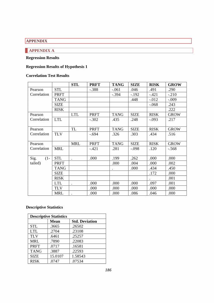
186
APPENDIX
APPENDIX A
Regression Results
Regression Results of Hypothesis 1
Correlation Test Results
STL PRFT TANG SIZE RISK GROW
Pearson
Correlation
STL -.388 -.061 .046 .491 .290
PRFT -.394 -.192 -.421 -.210
TANG .448 -.012 -.009
SIZE -.068 .243
RISK .222
Pearson
Correlation
LTL PRFT TANG SIZE RISK GROW
LTL -.302 .435 .248 -.093 .217
Pearson
Correlation
TL PRFT TANG SIZE RISK GROW
TLV -.694 .326 .303 .434 .516
Pearson
Correlation
MRL PRFT TANG SIZE RISK GROW
MRL -.421 .281 -.098 .120 -.568
Sig. (1-
tailed)
STL . .000 .199 .262 .000 .000
PRFT .000 .004 .000 .002
TANG . .000 .434 .450
SIZE .172 .000
RISK . .001
LTL . .000 .000 .000 .097 .001
TLV .000 .000 .000 .000 .000
MRL . .000 .000 .086 .046 .000
Descriptive Statistics
Descriptive Statistics
Mean Std. Deviation
STL .3665 .26502
LTL .2704 .23108
TLV .6461 .25257
MRL .7890 .22083
PRFT .0717 .16581
TANG .3887 .22593
SIZE 15.0107 1.58543
RISK .0747 .07534
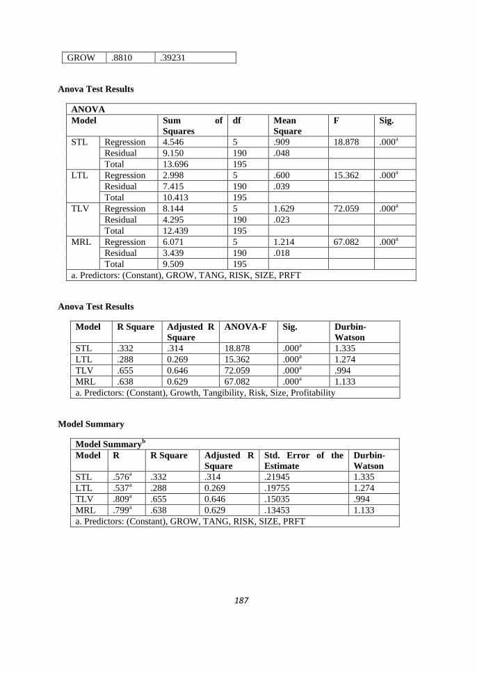
187
GROW .8810 .39231
Anova Test Results
ANOVA
Model Sum of
Squares
df Mean
Square
F Sig.
STL Regression 4.546 5 .909 18.878 .000a
Residual 9.150 190 .048
Total 13.696 195
LTL Regression 2.998 5 .600 15.362 .000a
Residual 7.415 190 .039
Total 10.413 195
TLV Regression 8.144 5 1.629 72.059 .000a
Residual 4.295 190 .023
Total 12.439 195
MRL Regression 6.071 5 1.214 67.082 .000a
Residual 3.439 190 .018
Total 9.509 195
a. Predictors: (Constant), GROW, TANG, RISK, SIZE, PRFT
Anova Test Results
Model R Square Adjusted R
Square
ANOVA-F Sig. Durbin-
Watson
STL .332 .314 18.878 .000a 1.335
LTL .288 0.269 15.362 .000a 1.274
TLV .655 0.646 72.059 .000a .994
MRL .638 0.629 67.082 .000a 1.133
a. Predictors: (Constant), Growth, Tangibility, Risk, Size, Profitability
Model Summary
Model Summaryb
Model R R Square Adjusted R
Square
Std. Error of the
Estimate
Durbin-
Watson
STL .576a .332 .314 .21945 1.335
LTL .537a .288 0.269 .19755 1.274
TLV .809a .655 0.646 .15035 .994
MRL .799a .638 0.629 .13453 1.133
a. Predictors: (Constant), GROW, TANG, RISK, SIZE, PRFT
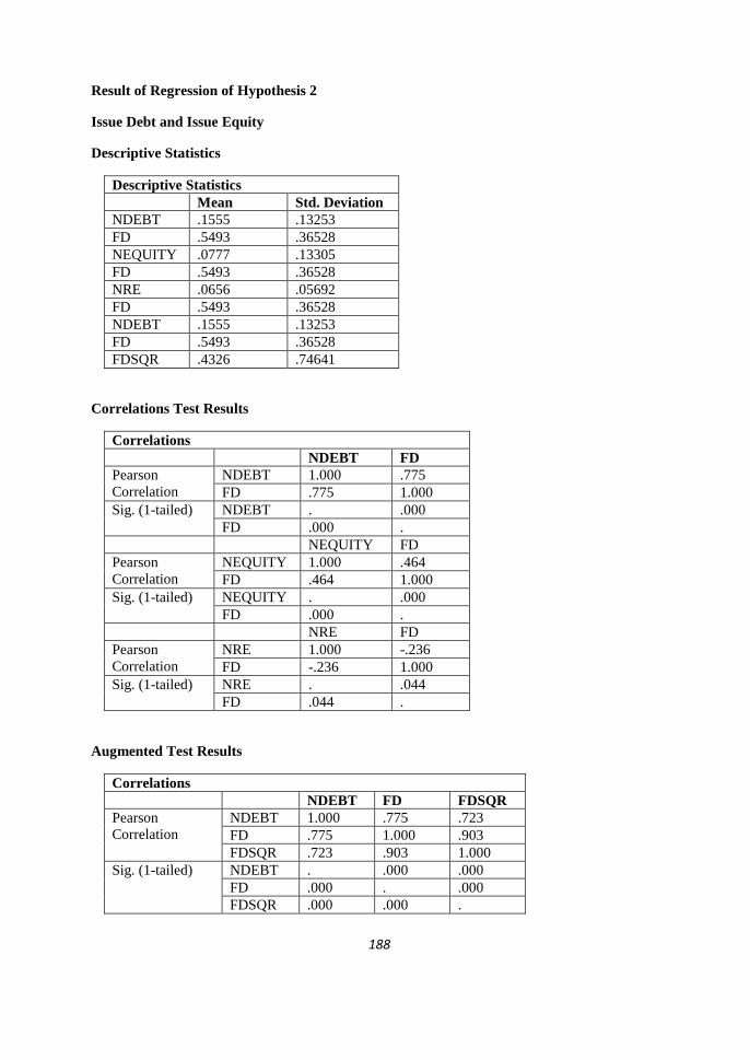
188
Result of Regression of Hypothesis 2
Issue Debt and Issue Equity
Descriptive Statistics
Descriptive Statistics
Mean Std. Deviation
NDEBT .1555 .13253
FD .5493 .36528
NEQUITY .0777 .13305
FD .5493 .36528
NRE .0656 .05692
FD .5493 .36528
NDEBT .1555 .13253
FD .5493 .36528
FDSQR .4326 .74641
Correlations Test Results
Correlations
NDEBT FD
Pearson
Correlation
NDEBT 1.000 .775
FD .775 1.000
Sig. (1-tailed) NDEBT . .000
FD .000 .
NEQUITY FD
Pearson
Correlation
NEQUITY 1.000 .464
FD .464 1.000
Sig. (1-tailed) NEQUITY . .000
FD .000 .
NRE FD
Pearson
Correlation
NRE 1.000 -.236
FD -.236 1.000
Sig. (1-tailed) NRE . .044
FD .044 .
Augmented Test Results
Correlations
NDEBT FD FDSQR
Pearson
Correlation
NDEBT 1.000 .775 .723
FD .775 1.000 .903
FDSQR .723 .903 1.000
Sig. (1-tailed) NDEBT . .000 .000
FD .000 . .000
FDSQR .000 .000 .
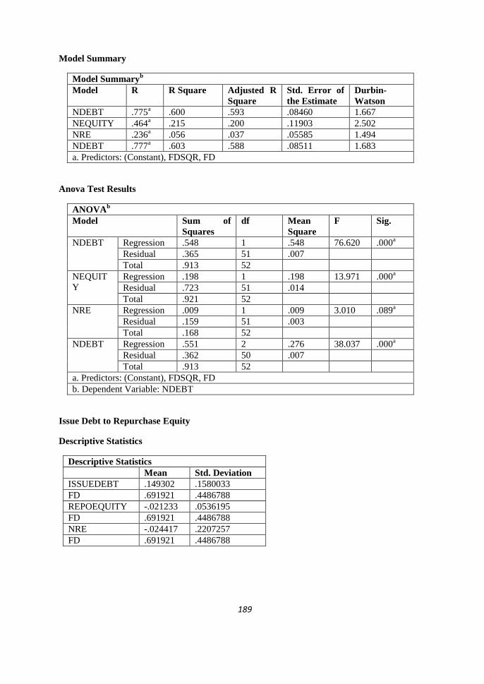
189
Model Summary
Model Summaryb
Model R R Square Adjusted R
Square
Std. Error of
the Estimate
Durbin-
Watson
NDEBT .775a .600 .593 .08460 1.667
NEQUITY .464a .215 .200 .11903 2.502
NRE .236a .056 .037 .05585 1.494
NDEBT .777a .603 .588 .08511 1.683
a. Predictors: (Constant), FDSQR, FD
Anova Test Results
ANOVAb
Model Sum of
Squares
df Mean
Square
F Sig.
NDEBT Regression .548 1 .548 76.620 .000a
Residual .365 51 .007
Total .913 52
NEQUIT
Y
Regression .198 1 .198 13.971 .000a
Residual .723 51 .014
Total .921 52
NRE Regression .009 1 .009 3.010 .089a
Residual .159 51 .003
Total .168 52
NDEBT Regression .551 2 .276 38.037 .000a
Residual .362 50 .007
Total .913 52
a. Predictors: (Constant), FDSQR, FD
b. Dependent Variable: NDEBT
Issue Debt to Repurchase Equity
Descriptive Statistics
Descriptive Statistics
Mean Std. Deviation
ISSUEDEBT .149302 .1580033
FD .691921 .4486788
REPOEQUITY -.021233 .0536195
FD .691921 .4486788
NRE -.024417 .2207257
FD .691921 .4486788
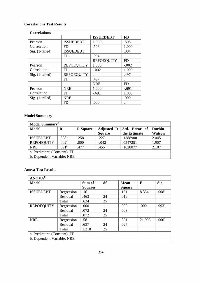
190
Correlations Test Results
Correlations
ISSUEDEBT FD
Pearson
Correlation
ISSUEDEBT 1.000 .508
FD .508 1.000
Sig. (1-tailed) ISSUEDEBT . .004
FD .004 .
REPOEQUITY FD
Pearson
Correlation
REPOEQUITY 1.000 -.002
FD -.002 1.000
Sig. (1-tailed) REPOEQUITY . .497
FD .497 .
NRE FD
Pearson
Correlation
NRE 1.000 -.691
FD -.691 1.000
Sig. (1-tailed) NRE . .000
FD .000 .
Model Summary
Model Summaryb
Model R R Square Adjusted R
Square
Std. Error of
the Estimate
Durbin-
Watson
ISSUEDEBT .508a .258 .227 .1388900 2.045
REPOEQUITY .002a .000 -.042 .0547251 1.907
NRE .691a .477 .455 .1628877 2.187
a. Predictors: (Constant), FD
b. Dependent Variable: NRE
Anova Test Results
ANOVAb
Model Sum of
Squares
df Mean
Square
F Sig.
ISSUEDEBT Regression .161 1 .161 8.354 .008a
Residual .463 24 .019
Total .624 25
REPOEQUITY Regression .000 1 .000 .000 .993a
Residual .072 24 .003
Total .072 25
NRE Regression .581 1 .581 21.906 .000a
Residual .637 24 .027
Total 1.218 25
a. Predictors: (Constant), FD
b. Dependent Variable: NRE
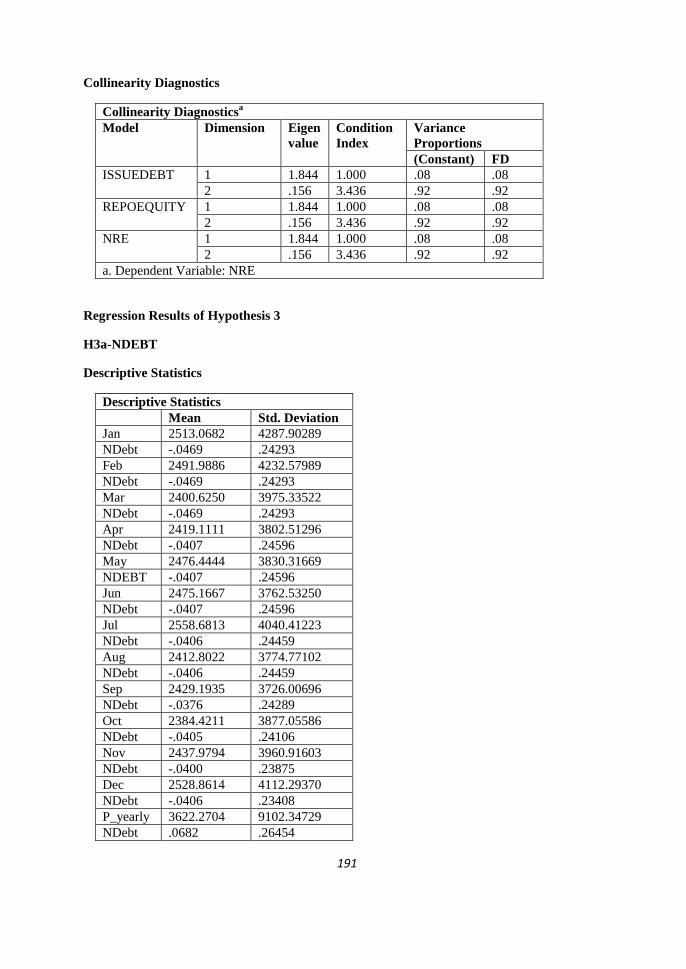
191
Collinearity Diagnostics
Collinearity Diagnosticsa
Model Dimension Eigen
value
Condition
Index
Variance
Proportions
(Constant) FD
ISSUEDEBT 1 1.844 1.000 .08 .08
2 .156 3.436 .92 .92
REPOEQUITY 1 1.844 1.000 .08 .08
2 .156 3.436 .92 .92
NRE 1 1.844 1.000 .08 .08
2 .156 3.436 .92 .92
a. Dependent Variable: NRE
Regression Results of Hypothesis 3
H3a-NDEBT
Descriptive Statistics
Descriptive Statistics
Mean Std. Deviation
Jan 2513.0682 4287.90289
NDebt -.0469 .24293
Feb 2491.9886 4232.57989
NDebt -.0469 .24293
Mar 2400.6250 3975.33522
NDebt -.0469 .24293
Apr 2419.1111 3802.51296
NDebt -.0407 .24596
May 2476.4444 3830.31669
NDEBT -.0407 .24596
Jun 2475.1667 3762.53250
NDebt -.0407 .24596
Jul 2558.6813 4040.41223
NDebt -.0406 .24459
Aug 2412.8022 3774.77102
NDebt -.0406 .24459
Sep 2429.1935 3726.00696
NDebt -.0376 .24289
Oct 2384.4211 3877.05586
NDebt -.0405 .24106
Nov 2437.9794 3960.91603
NDebt -.0400 .23875
Dec 2528.8614 4112.29370
NDebt -.0406 .23408
P_yearly 3622.2704 9102.34729
NDebt .0682 .26454
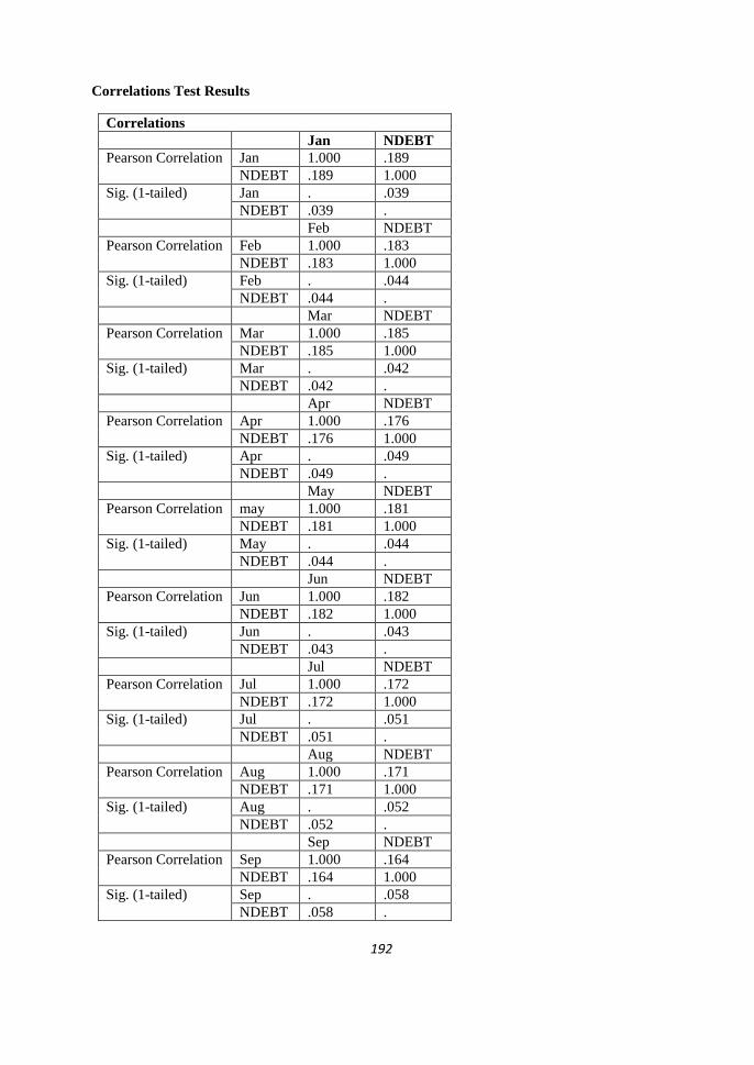
192
Correlations Test Results
Correlations
Jan NDEBT
Pearson Correlation Jan 1.000 .189
NDEBT .189 1.000
Sig. (1-tailed) Jan . .039
NDEBT .039 .
Feb NDEBT
Pearson Correlation Feb 1.000 .183
NDEBT .183 1.000
Sig. (1-tailed) Feb . .044
NDEBT .044 .
Mar NDEBT
Pearson Correlation Mar 1.000 .185
NDEBT .185 1.000
Sig. (1-tailed) Mar . .042
NDEBT .042 .
Apr NDEBT
Pearson Correlation Apr 1.000 .176
NDEBT .176 1.000
Sig. (1-tailed) Apr . .049
NDEBT .049 .
May NDEBT
Pearson Correlation may 1.000 .181
NDEBT .181 1.000
Sig. (1-tailed) May . .044
NDEBT .044 .
Jun NDEBT
Pearson Correlation Jun 1.000 .182
NDEBT .182 1.000
Sig. (1-tailed) Jun . .043
NDEBT .043 .
Jul NDEBT
Pearson Correlation Jul 1.000 .172
NDEBT .172 1.000
Sig. (1-tailed) Jul . .051
NDEBT .051 .
Aug NDEBT
Pearson Correlation Aug 1.000 .171
NDEBT .171 1.000
Sig. (1-tailed) Aug . .052
NDEBT .052 .
Sep NDEBT
Pearson Correlation Sep 1.000 .164
NDEBT .164 1.000
Sig. (1-tailed) Sep . .058
NDEBT .058 .
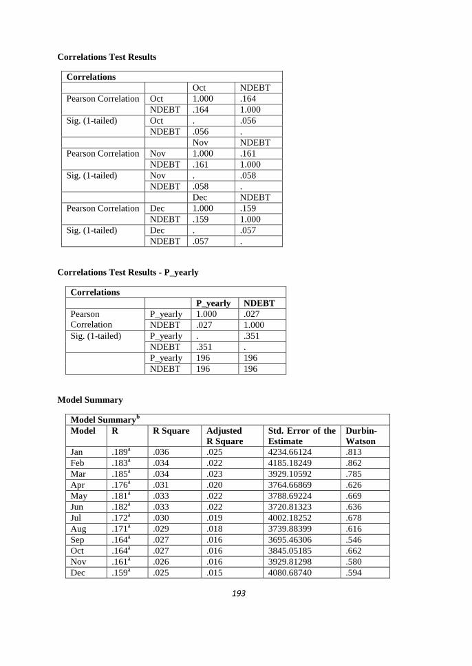
193
Correlations Test Results
Correlations
Oct NDEBT
Pearson Correlation Oct 1.000 .164
NDEBT .164 1.000
Sig. (1-tailed) Oct . .056
NDEBT .056 .
Nov NDEBT
Pearson Correlation Nov 1.000 .161
NDEBT .161 1.000
Sig. (1-tailed) Nov . .058
NDEBT .058 .
Dec NDEBT
Pearson Correlation Dec 1.000 .159
NDEBT .159 1.000
Sig. (1-tailed) Dec . .057
NDEBT .057 .
Correlations Test Results - P_yearly
Correlations
P_yearly NDEBT
Pearson
Correlation
P_yearly 1.000 .027
NDEBT .027 1.000
Sig. (1-tailed) P_yearly . .351
NDEBT .351 .
P_yearly 196 196
NDEBT 196 196
Model Summary
Model Summaryb
Model R R Square Adjusted
R Square
Std. Error of the
Estimate
Durbin-
Watson
Jan .189a .036 .025 4234.66124 .813
Feb .183a .034 .022 4185.18249 .862
Mar .185a .034 .023 3929.10592 .785
Apr .176a .031 .020 3764.66869 .626
May .181a .033 .022 3788.69224 .669
Jun .182a .033 .022 3720.81323 .636
Jul .172a .030 .019 4002.18252 .678
Aug .171a .029 .018 3739.88399 .616
Sep .164a .027 .016 3695.46306 .546
Oct .164a .027 .016 3845.05185 .662
Nov .161a .026 .016 3929.81298 .580
Dec .159a .025 .015 4080.68740 .594

194
Yearly .027a .001 -.004 9122.33323 1.558
a. Predictors: (Constant), NDEBT
b. Dependent Variable: P_yearly
Anova Test Results
Model Sum of
Squares
df Mean
Square
F Sig.
Jan
Regression 5.741E7 1 5.741E7 3.201 .077a
Residual 1.542E9 86 1.793E7
Total 1.600E9 87
Feb
Regression 5.223E7 1 5.223E7 2.982 .088a
Residual 1.506E9 86 1.752E7
Total 1.559E9 87
Mar
Regression 4.723E7 1 4.723E7 3.059 .084a
Residual 1.328E9 86 1.544E7
Total 1.375E9 87
Apr
Regression 3.966E7 1 3.966E7 2.798 .098a
Residual 1.247E9 88 1.417E7
Total 1.287E9 89
May
Regression 4.258E7 1 4.258E7 2.966 .089a
Residual 1.263E9 88 1.435E7
Total 1.306E9 89
Jun
Regression 4.163E7 1 4.163E7 3.007 .086a
Residual 1.218E9 88 1.384E7
Total 1.260E9 89
Jul
Regression 4.369E7 1 4.369E7 2.728 .102a
Residual 1.426E9 89 1.602E7
Total 1.469E9 90
Aug
Regression 3.758E7 1 3.758E7 2.687 .105a
Residual 1.245E9 89 1.399E7
Total 1.282E9 90
Sep
Regression 3.451E7 1 3.451E7 2.527 .115a
Residual 1.243E9 91 1.366E7
Total 1.277E9 92
Oct
Regression 3.802E7 1 3.802E7 2.571 .112a
Residual 1.375E9 93 1.478E7
Total 1.413E9 94
Nov
Regression 3.900E7 1 3.900E7 2.526 .115a
Residual 1.467E9 95 1.544E7
Total 1.506E9 96
Dec
Regression 4.255E7 1 4.255E7 2.555 .113a
Residual 1.649E9 99 1.665E7
Total 1.691E9 100
Yearly
Regression 1.219E7 1 1.219E7 .146 .702a
Residual 1.614E10 194 8.322E7
Total 1.616E10 195
a. Predictors: (Constant), NDEBT

195
b. Dependent Variable: P_yearly
H3b-NEQUITY
Descriptive Statistics
Descriptive Statistics
Mean Std. Deviation
Jan 2513.0682 4287.90289
NEQUITY .0317 .14489
Feb 2491.9886 4232.57989
NEQUITY .0317 .14489
Mar 2400.6250 3975.33522
NEQUITY .0317 .14489
Apr 2419.1111 3802.51296
NEQUITY .0324 .14360
May 2476.4444 3830.31669
NEQUITY .0324 .14360
Jun 2475.1667 3762.53250
NEQUITY .0324 .14360
Jul 2558.6813 4040.41223
NEQUITY .0363 .14761
Aug 2412.8022 3774.77102
NEQUITY .0363 .14761
Sep 2429.1935 3726.00696
NEQUITY .0357 .14605
Oct 2384.4211 3877.05586
NEQUITY .0352 .14454
Nov 2437.9794 3960.91603
NEQUITY .0341 .14324
Dec 2528.8614 4112.29370
NEQUITY .0327 .14062
P_yearly 3622.2704 9102.34729
NEQUITY .0458 .13826
Correlations Test Results
Correlations
Jan NEQUIT
Y
Pearson Correlation Jan 1.000 -.067
NEQUIT
Y
-.067 1.000
Sig. (1-tailed) Jan . .266
NEQUIT
Y
.266 .
Feb NEQUITY

196
Pearson Correlation Feb 1.000 -.066
NEQUIT
Y
-.066 1.000
Sig. (1-tailed) Feb . .269
NEQUIT
Y
.269 .
Mar NEQUITY
Pearson Correlation Mar 1.000 -.067
NEQUIT
Y
-.067 1.000
Sig. (1-tailed) Mar . .268
NEQUIT
Y
.268 .
Apr NEQUITY
Pearson Correlation Apr 1.000 -.067
NEQUIT
Y
-.067 1.000
Sig. (1-tailed) Apr . .265
NEQUIT
Y
.265 .
May NEQUITY
Pearson Correlation May 1.000 -.066
NEQUIT
Y
-.066 1.000
Sig. (1-tailed) May . .267
NEQUIT
Y
.267 .
Jun NEQUITY
Pearson Correlation Jun 1.000 -.067
NEQUIT
Y
-.067 1.000
Sig. (1-tailed) Jun . .265
NEQUIT
Y
.265 .
Jul NEQUITY
Pearson Correlation Jul 1.000 -.080
NEQUIT
Y
-.080 1.000
Sig. (1-tailed) Jul . .227
NEQUIT
Y
.227 .
Aug NEQUITY
Pearson Correlation Aug 1.000 -.079
NEQUIT
Y
-.079 1.000
Sig. (1-tailed) Aug . .230
NEQUIT
Y
.230 .
Sep NEQUITY
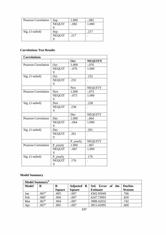
197
Pearson Correlation Sep 1.000 -.082
NEQUIT
Y
-.082 1.000
Sig. (1-tailed) Sep . .217
NEQUIT
Y
.217 .
Correlations Test Results
Correlations
Oct NEQUITY
Pearson Correlation Oct 1.000 -.076
NEQUIT
Y
-.076 1.000
Sig. (1-tailed) Oct . .232
NEQUIT
Y
.232 .
Nov NEQUITY
Pearson Correlation Nov 1.000 -.073
NEQUIT
Y
-.073 1.000
Sig. (1-tailed) Nov . .238
NEQUIT
Y
.238 .
Dec NEQUITY
Pearson Correlation Dec 1.000 -.064
NEQUIT
Y
-.064 1.000
Sig. (1-tailed) Dec . .261
NEQUIT
Y
.261 .
P_yearly NEQUITY
Pearson Correlation P_yearly 1.000 -.067
NEQUIT
Y
-.067 1.000
Sig. (1-tailed) P_yearly . .176
NEQUIT
Y
.176 .
Model Summary
Model Summaryb
Model R R
Square
Adjusted R
Square
Std. Error of the
Estimate
Durbin-
Watson
Jan .067a .005 -.007 4302.95049 .766
Feb .066a .004 -.007 4247.73093 .820
Mar .067a .004 -.007 3989.42032 .742
Apr .067a .005 -.007 3815.42095 .600

198
May .066a .004 -.007 3843.54969 .638
Jun .067a .004 -.007 3775.32764 .610
Jul .080a .006 -.005 4050.18176 .659
Aug .079a .006 -.005 3784.18677 .596
Sep .082a .007 -.004 3733.72683 .532
Oct .076a .006 -.005 3886.60177 .652
Nov .073a .005 -.005 3970.99520 .567
Dec .064a .004 -.006 4124.44223 .586
yearly .067a .004 .000 9105.34743 1.574
a. Predictors: (Constant), NEQUITY
b. Dependent Variable: P_yearly
Anova Test Results
ANOVAb
Model Sum of
Squares
df Mean Square F Sig.
Jan
Regression 7268743.051 1 7268743.051 .393 .533a
Residual 1.592E9 86 1.852E7
Total 1.600E9 87
Feb
Regression 6864970.917 1 6864970.917 .380 .539a
Residual 1.552E9 86 1.804E7
Total 1.559E9 87
Mar
Regression 6155433.770 1 6155433.770 .387 .536a
Residual 1.369E9 86 1.592E7
Total 1.375E9 87
Apr
Regression 5805872.844 1 5805872.844 .399 .529a
Residual 1.281E9 88 1.456E7
Total 1.287E9 89
May
Regression 5735080.005 1 5735080.005 .388 .535a
Residual 1.300E9 88 1.477E7
Total 1.306E9 89
Jun
Regression 5669226.872 1 5669226.872 .398 .530a
Residual 1.254E9 88 1.425E7
Total 1.260E9 89
Jul
Regression 9290256.505 1 9290256.505 .566 .454a
Residual 1.460E9 89 1.640E7
Total 1.469E9 90
Aug
Regression 7914473.120 1 7914473.120 .553 .459a
Residual 1.274E9 89 1.432E7
Total 1.282E9 90
Sep
Regression 8642603.153 1 8642603.153 .620 .433a
Residual 1.269E9 91 1.394E7
Total 1.277E9 92
Oct
Regression 8139221.850 1 8139221.850 .539 .465a
Residual 1.405E9 93 1.511E7
Total 1.413E9 94
Regression 8093885.404 1 8093885.404 .513 .475a

199
Nov Residual 1.498E9 95 1.577E7
Total 1.506E9 96
Dec
Regression 7004597.840 1 7004597.840 .412 .523a
Residual 1.684E9 99 1.701E7
Total 1.691E9 100
Yearly
Regression 7.226E7 1 7.226E7 .872 .352a
Residual 1.608E10 194 8.291E7
Total 1.616E10 195
a. Predictors: (Constant), NEQUITY
b. Dependent Variable: P_yearly
H3c-Issue Debt to Repurchase Equity
Descriptive Statistics
Descriptive Statistics
Mean Std. Deviation
Jan 6826.666667 9.1839548E3
NDEBT .071248 .0655959
NEQUITY -.020687 .0301779
Feb 6771.111111 9.2494111E3
NDEBT .071248 .0655959
NEQUITY -.020687 .0301779
Mar 6340.000000 8.2777952E3
NDEBT .071248 .0655959
NEQUITY -.020687 .0301779
Apr 6107.222222 7.4446869E3
NDEBT .071248 .0655959
NEQUITY -.020687 .0301779
May 5984.444444 7.4346118E3
NDEBT .071248 .0655959
NEQUITY -.020687 .0301779
Jun 5695.000000 6.9278947E3
NDEBT .071248 .0655959
NEQUITY -.020687 .0301779
Jul 6130.000000 7.8145341E3
NDEBT .071248 .0655959
NEQUITY -.020687 .0301779
Aug 5909.444444 7.2999030E3
NDEBT .071248 .0655959
NEQUITY -.020687 .0301779
Sep 5592.222222 6.6337170E3
NDEBT .071248 .0655959
NEQUITY -.020687 .0301779
Oct 4705.000000 5.5191842E3
NDEBT .071248 .0655959
NEQUITY -.020687 .0301779
Nov 5206.111111 6.2086285E3

200
NDEBT .071248 .0655959
NEQUITY -.020687 .0301779
Dec 4867.000000 6.0052825E3
NDEBT .064430 .0654957
NEQUITY -.023205 .0295450
P_yearly 4358.695652 5.7944408E3
NDEBT .163867 .1622490
NEQUITY -.022900 .0567996
Correlations Test Results
Correlations
Jan NDEBT NEQUITY
Pearson
Correlation
Jan 1.000 -.347 .407
NDEBT -.347 1.000 -.825
NEQUITY .407 -.825 1.000
Sig. (1-tailed) Jan . .180 .138
NDEBT .180 . .003
NEQUITY .138 .003 .
Feb NDEBT NEQUITY
Pearson
Correlation
Feb 1.000 -.352 .401
NDEBT -.352 1.000 -.825
NEQUITY .401 -.825 1.000
Sig. (1-tailed) Feb . .176 .142
NDEBT .176 . .003
NEQUITY .142 .003 .
Mar NDEBT NEQUITY
Pearson
Correlation
Mar 1.000 -.351 .442
NDEBT -.351 1.000 -.825
NEQUITY .442 -.825 1.000
Sig. (1-tailed) Mar . .177 .117
NDEBT .177 . .003
NEQUITY .117 .003 .
Apr NDEBT NEQUITY
Pearson
Correlation
Apr 1.000 -.343 .471
NDEBT -.343 1.000 -.825
NEQUITY .471 -.825 1.000
Sig. (1-tailed) Apr . .183 .100
NDEBT .183 . .003
NEQUITY .100 .003 .
May NDEBT NEQUITY
Pearson
Correlation
May 1.000 -.343 .441
NDEBT -.343 1.000 -.825
NEQUITY .441 -.825 1.000
Sig. (1-tailed) May . .183 .118
NDEBT .183 . .003
NEQUITY .118 .003 .
Jun NDEBT NEQUITY
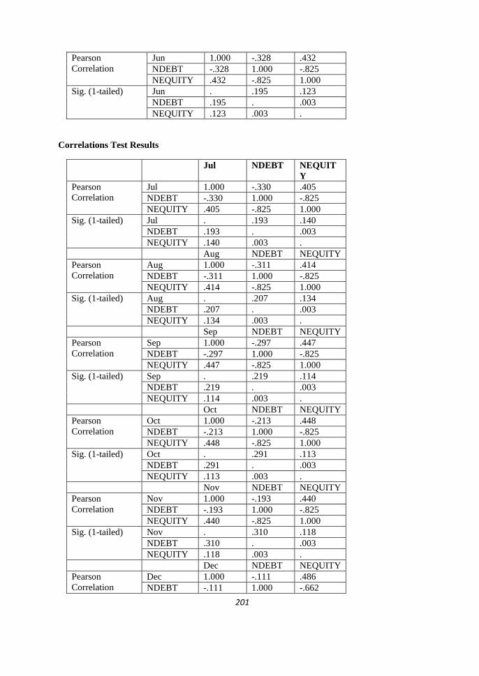
201
Pearson
Correlation
Jun 1.000 -.328 .432
NDEBT -.328 1.000 -.825
NEQUITY .432 -.825 1.000
Sig. (1-tailed) Jun . .195 .123
NDEBT .195 . .003
NEQUITY .123 .003 .
Correlations Test Results
Jul NDEBT NEQUIT
Y
Pearson
Correlation
Jul 1.000 -.330 .405
NDEBT -.330 1.000 -.825
NEQUITY .405 -.825 1.000
Sig. (1-tailed) Jul . .193 .140
NDEBT .193 . .003
NEQUITY .140 .003 .
Aug NDEBT NEQUITY
Pearson
Correlation
Aug 1.000 -.311 .414
NDEBT -.311 1.000 -.825
NEQUITY .414 -.825 1.000
Sig. (1-tailed) Aug . .207 .134
NDEBT .207 . .003
NEQUITY .134 .003 .
Sep NDEBT NEQUITY
Pearson
Correlation
Sep 1.000 -.297 .447
NDEBT -.297 1.000 -.825
NEQUITY .447 -.825 1.000
Sig. (1-tailed) Sep . .219 .114
NDEBT .219 . .003
NEQUITY .114 .003 .
Oct NDEBT NEQUITY
Pearson
Correlation
Oct 1.000 -.213 .448
NDEBT -.213 1.000 -.825
NEQUITY .448 -.825 1.000
Sig. (1-tailed) Oct . .291 .113
NDEBT .291 . .003
NEQUITY .113 .003 .
Nov NDEBT NEQUITY
Pearson
Correlation
Nov 1.000 -.193 .440
NDEBT -.193 1.000 -.825
NEQUITY .440 -.825 1.000
Sig. (1-tailed) Nov . .310 .118
NDEBT .310 . .003
NEQUITY .118 .003 .
Dec NDEBT NEQUITY
Pearson
Correlation
Dec 1.000 -.111 .486
NDEBT -.111 1.000 -.662

202
NEQUITY .486 -.662 1.000
Sig. (1-tailed) Dec . .380 .077
NDEBT .380 . .019
NEQUITY .077 .019 .
P_yearly NDEBT NEQUITY
Pearson
Correlation
P_yearly 1.000 -.292 .223
NDEBT -.292 1.000 -.041
NEQUITY .223 -.041 1.000
Sig. (1-tailed) P_yearly . .088 .154
NDEBT .088 . .426
NEQUITY .154 .426 .
Anova Test Results
ANOVAb
Model Sum of
Squares
df Mean Square F Sig.
Jan Regression 1.120E8 2 5.602E7 .597 .580a
Residual 5.627E8 6 9.379E7
Total 6.748E8 8
Feb Regression 1.111E8 2 5.554E7 .581 .588a
Residual 5.733E8 6 9.556E7
Total 6.844E8 8
Mar Regression 1.076E8 2 5.378E7 .732 .519a
Residual 4.406E8 6 7.344E7
Total 5.482E8 8
Apr Regression 1.013E8 2 5.067E7 .889 .459a
Residual 3.420E8 6 5.701E7
Total 4.434E8 8
May Regression 8.636E7 2 4.318E7 .728 .521a
Residual 3.558E8 6 5.930E7
Total 4.422E8 8
Jun Regression 7.276E7 2 3.638E7 .701 .532a
Residual 3.112E8 6 5.187E7
Total 3.840E8 8
Jul Regression 8.005E7 2 4.003E7 .588 .585a
Residual 4.085E8 6 6.808E7
Total 4.885E8 8
Aug Regression 7.434E7 2 3.717E7 .634 .563a
Residual 3.520E8 6 5.866E7
Total 4.263E8 8
Sep Regression 7.588E7 2 3.794E7 .824 .483a
Residual 2.762E8 6 4.603E7
Total 3.520E8 8

203
Anova Test Results
ANOVAb
Oct Regression 6.774E7 2 3.387E7 1.155 .376a
Residual 1.760E8 6 2.933E7
Total 2.437E8 8
Nov Regression 8.782E7 2 4.391E7 1.195 .366a
Residual 2.206E8 6 3.676E7
Total 3.084E8 8
Dec Regression 1.020E8 2 5.100E7 1.604 .267a
Residual 2.226E8 7 3.180E7
Total 3.246E8 9
yearly Regression 9.586E7 2 4.793E7 1.491 .249a
Residual 6.428E8 20 3.214E7
Total 7.387E8 22
a. Predictors: (Constant), NEQUITY, NDEBT
b. Dependent Variable: P_yearly
Model Summary
Model Summaryb
Model R R Square Adjusted R
Square
Std. Error of the
Estimate
Durbin-
Watson
Jan .407a .166 -.112 9.6842906E3 .987
Feb .403a .162 -.117 9.7752614E3 1.049
Mar .443a .196 -.072 8.5694609E3 .890
Apr .478a .229 -.029 7.5502543E3 .684
May .442a .195 -.073 7.7009209E3 .813
Jun .435a .189 -.081 7.2019407E3 .762
Jul .405a .164 -.115 8.2510944E3 .868
Aug .418a .174 -.101 7.6591030E3 .754
Sep .464a .216 -.046 6.7843834E3 .598
Oct .527a .278 .037 5.4152935E3 .806
Nov .534a .285 .046 6.0629603E3 .800
Dec .561a .314 .118 5.6388036E3 .888
yearly .360a .130 .043 5.6692401E3 1.577
a. Predictors: (Constant), REPOEQUITY, NDEBT
b. Dependent Variable: P_yearly
Regression Results of Hypothesis 4
Growth and Mature Firms
Descriptive Statistics
Sum Mean Sum Mean
LTL_G 46.10 0.3136 LTL_M 20.49 0.2029
FIXAS_G 68.56 0.4664 FIXAS_M 28.43 0.2815
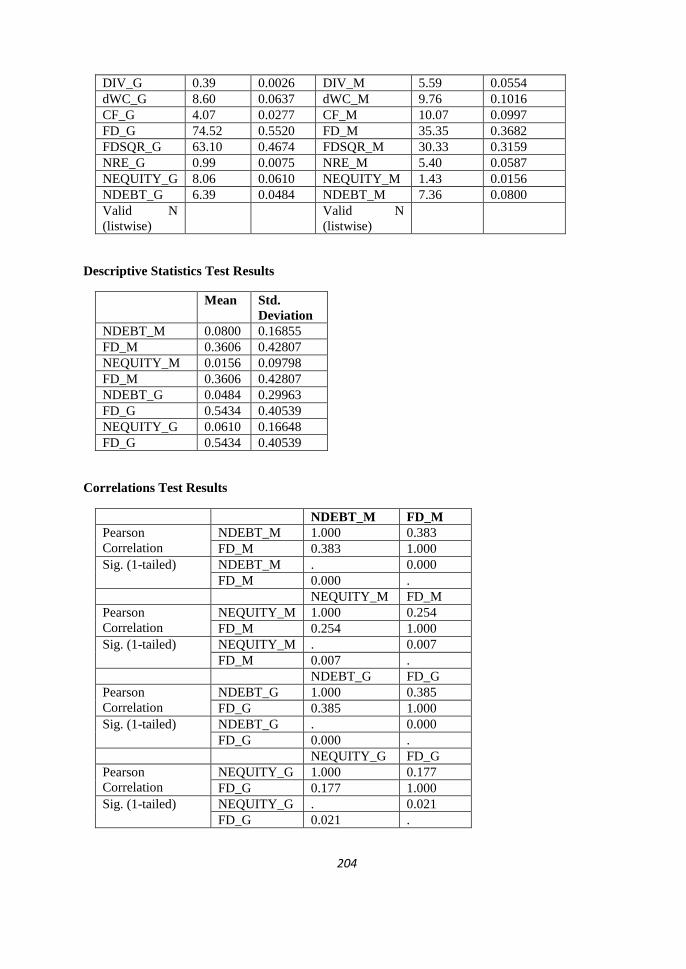
204
DIV_G 0.39 0.0026 DIV_M 5.59 0.0554
dWC_G 8.60 0.0637 dWC_M 9.76 0.1016
CF_G 4.07 0.0277 CF_M 10.07 0.0997
FD_G 74.52 0.5520 FD_M 35.35 0.3682
FDSQR_G 63.10 0.4674 FDSQR_M 30.33 0.3159
NRE_G 0.99 0.0075 NRE_M 5.40 0.0587
NEQUITY_G 8.06 0.0610 NEQUITY_M 1.43 0.0156
NDEBT_G 6.39 0.0484 NDEBT_M 7.36 0.0800
Valid N
(listwise)
Valid N
(listwise)
Descriptive Statistics Test Results
Mean Std.
Deviation
NDEBT_M 0.0800 0.16855
FD_M 0.3606 0.42807
NEQUITY_M 0.0156 0.09798
FD_M 0.3606 0.42807
NDEBT_G 0.0484 0.29963
FD_G 0.5434 0.40539
NEQUITY_G 0.0610 0.16648
FD_G 0.5434 0.40539
Correlations Test Results
NDEBT_M FD_M
Pearson
Correlation
NDEBT_M 1.000 0.383
FD_M 0.383 1.000
Sig. (1-tailed) NDEBT_M . 0.000
FD_M 0.000 .
NEQUITY_M FD_M
Pearson
Correlation
NEQUITY_M 1.000 0.254
FD_M 0.254 1.000
Sig. (1-tailed) NEQUITY_M . 0.007
FD_M 0.007 .
NDEBT_G FD_G
Pearson
Correlation
NDEBT_G 1.000 0.385
FD_G 0.385 1.000
Sig. (1-tailed) NDEBT_G . 0.000
FD_G 0.000 .
NEQUITY_G FD_G
Pearson
Correlation
NEQUITY_G 1.000 0.177
FD_G 0.177 1.000
Sig. (1-tailed) NEQUITY_G . 0.021
FD_G 0.021 .

205
Model Summary
Model R R
Square
Adjusted
R Square
Std. Error of
the Estimate
Durbin-
Watson
NDEBT_M 0.383a 0.147 0.137 0.15657 1.602
NEQUITY_M 0.254a 0.064 0.054 0.09529 2.284
NDEBT_G 0.385a 0.148 0.141 0.27766 1.670
NEQUITY_G 0.177a 0.031 0.024 0.16448 2.108
a. Predictors: (Constant), FD_G
Model Summary
Model R R
Square
Adjusted
R Square
Std. Error of
the Estimate
Durbin-
Watson
NDEBT_M 0.495a 0.245 0.229 0.14804 1.486
NDEBT_G 0.533a 0.285 0.273 0.25540 1.822
a. Predictors: (Constant), FDSQR_G, FD_G and M
b. Dependent Variable: NDEBT_G and M
Anova Test Results
Model Sum of
Squares
df Mean
Square
F Sig.
NDEBT_M Regression 0.379 1 0.379 15.463 0.000a
Residual 2.206 90 0.025
Total 2.585 91
NEQUITY_M Regression 0.056 1 0.056 6.196 0.015a
Residual 0.817 90 0.009
Total 0.874 91
NDEBT_G Regression 1.739 1 1.739 22.556 0.000a
Residual 10.022 130 0.077
Total 11.761 131
NEQUITY_G Regression .114 1 0.114 4.219 0.042a
Residual 3.517 130 0.027
Total 3.631 131
a. Predictors: (Constant), FD_G

206
APPENDIX B
List of Acronyms
Table B.1. Name of Firms
Name of Firms Acronyms
ASII Astra International
AUTO Astra Otoparts
ADMG Polychem Indonesia
BRPT Barito Pacific
BUDI Budi Acid Jaya
CPIN Charoen Pokphand Indonesia
DNKS Dankos Laboratories
FASW Fajar Surya Wisesa
GGRM Gudang Garam
GJTL Gajah Tunggal
HMSP Hanjaya Mandala Sampoerna
INAF Indofarma
INDF Indocement Tunggal Prakasa
INDR Indorama Synthetics
INKP Indah Kiat Pulp and Paper
INTP Indocement Tunggal Prakasa
KAEF Kimia Farma
KLBF Kalbe Farma
KOMI Komatsu Indonesia
RMBA Bentoel International Investama
SMCB Holcim Indonesia
SMGR Semen Gresik (Persero)
TKIM Pabrik Kertas Tjiwi Kimia
TSPC Tempo Scan Pacific
UNVR Unilever Indonesia
SULI Sumalindo Lestari Jaya
Table B.2. Variables and Its Sub-variables of Research
Variables of Research Acronyms
Aug August‟ stock price
Apr April‟ stock price
CAPEX Capital expenditures
CF Operating cash flow (after interest and taxes)
CF_M Cash flow of mature firm
CF_G Cash flow of growth firm
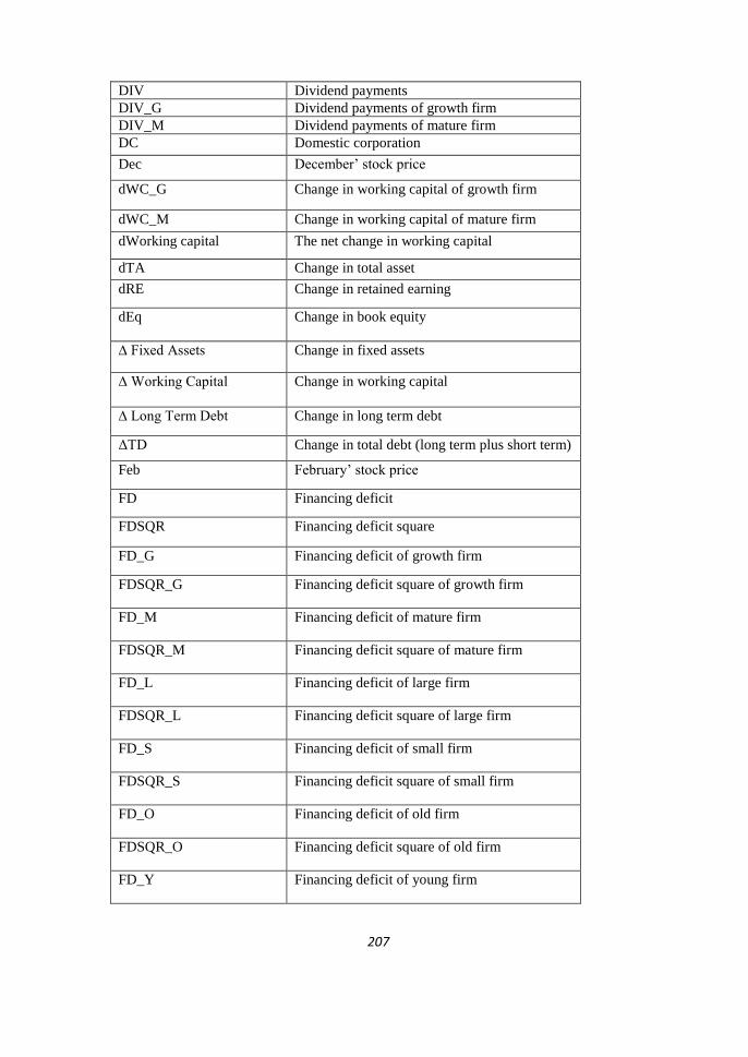
207
DIV Dividend payments
DIV_G Dividend payments of growth firm
DIV_M Dividend payments of mature firm
DC Domestic corporation
Dec December‟ stock price
dWC_G Change in working capital of growth firm
dWC_M Change in working capital of mature firm
dWorking capital The net change in working capital
dTA Change in total asset
dRE Change in retained earning
dEq Change in book equity
∆ Fixed Assets Change in fixed assets
∆ Working Capital Change in working capital
∆ Long Term Debt Change in long term debt
ΔTD Change in total debt (long term plus short term)
Feb February‟ stock price
FD Financing deficit
FDSQR Financing deficit square
FD_G Financing deficit of growth firm
FDSQR_G Financing deficit square of growth firm
FD_M Financing deficit of mature firm
FDSQR_M Financing deficit square of mature firm
FD_L Financing deficit of large firm
FDSQR_L Financing deficit square of large firm
FD_S Financing deficit of small firm
FDSQR_S Financing deficit square of small firm
FD_O Financing deficit of old firm
FDSQR_O Financing deficit square of old firm
FD_Y Financing deficit of young firm

208
FDSQR_Y Financing deficit square of young firm
FIXAS_G Fixed asset of growth firm
FIXAS_M Fixed asset of mature firm
GCC countries Gulf Cooperation Council (GCC) countries
Growth Growth firm
GROW Growth
Jan January‟ stock price
JM Jensen and Meckling
Jun June‟ stock price
Jul July‟ stock price
LTL_M Long-term leverage of mature firm
LTL_G Long-term leverage of growth firm
LTD payment Long-term debt payment
Large Large firm
LTL Long-term leverage
May May‟ stock price
MRL Market leverage
MM The Modigliani-Miller
MNC Multi National Corporation
Mature Mature firm
Mar March‟ stock price
MV of equity Market value of equity
NDEBT_G Net debt issue of growth firm
NEQUITY_G Net equity issue of growth firm
NDEBT_M Net debt issue of mature firm
NEQUITY_M Net equity issue of mature firm

209
NRE_G Newly retained earning of growth firm
NRE_M Newly retained earning of mature firm
NDEBT_L Net debt issue of large firm
NEQUITY_L Net equity issue of large firm
NRE_L Newly retained earning of large firm
NDEBT_S Net debt issue of small firm
NEQUITY_S Net equity issue of small firm
NRE_S Newly retained earning of small firm
NDEBT_O Net debt issue of old firm
NEQUITY_O Net equity issue of old firm
NRE_O Newly retained earning of old firm
NDEBT_Y Net debt issue of young firm
NEQUITY_Y Net equity issue of young firm
NRE_Y Newly retained earning of young firm
Net debtit Net debt issued in period t scaled by total assets
at the beginning of period t (assett-1)
Net debtt Long-term debt issuance at t minus long-term
debt reduction at t divided by total assets at t-1.
NPV Net present value
Nov November‟ stock price
NDEBT Net debt issue
NEQUITY Net equity issue
NRE Newly retained earning
Oct October‟ stock price
Old Old firm
P_Yearly Yearly stock price
PRFT Profitability
POT Pecking order theory
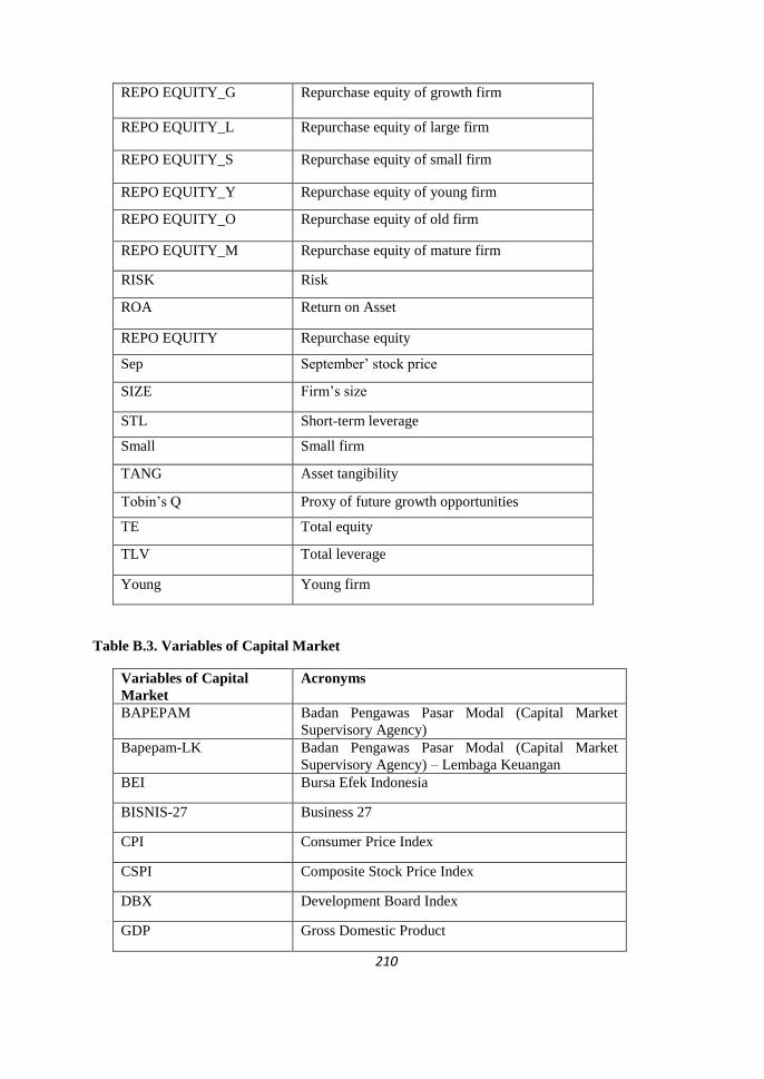
210
REPO EQUITY_G Repurchase equity of growth firm
REPO EQUITY_L Repurchase equity of large firm
REPO EQUITY_S Repurchase equity of small firm
REPO EQUITY_Y Repurchase equity of young firm
REPO EQUITY_O Repurchase equity of old firm
REPO EQUITY_M Repurchase equity of mature firm
RISK Risk
ROA Return on Asset
REPO EQUITY Repurchase equity
Sep September‟ stock price
SIZE Firm‟s size
STL Short-term leverage
Small Small firm
TANG Asset tangibility
Tobin‟s Q Proxy of future growth opportunities
TE Total equity
TLV Total leverage
Young Young firm
Table B.3. Variables of Capital Market
Variables of Capital
Market
Acronyms
BAPEPAM Badan Pengawas Pasar Modal (Capital Market
Supervisory Agency)
Bapepam-LK Badan Pengawas Pasar Modal (Capital Market
Supervisory Agency) – Lembaga Keuangan
BEI Bursa Efek Indonesia
BISNIS-27 Business 27
CPI Consumer Price Index
CSPI Composite Stock Price Index
DBX Development Board Index
GDP Gross Domestic Product

211
ICT Information and communication technology
IDR Indonesian Rupiah
IDX Indonesia Stock Exchange
IPO Initial Public Offering
JATS Jakarta Automatic Trading System
JSX Jakarta Stock Exchange
Kompas 100 Index consists of 100 shares of Listed Companies
that are selected based on considerations of liquidity
and market capitalisation
LQ45 Index Liquid 45 Index
MBX Main Board Index
MUI The Majelis Ulama Indonesia (the Sharia
Supervisory Board)
No.Kep-86/PM/1996 Nomor Keputusan-86/Pasar Modal/1996
PEFINDO-25 Pemeringkat Efek Indonesia 25 (rating agencies)
PT Perusahaan terbatas
KEHATI Sustainable Responsible Investment-Indonesian
Biodiversity Foundation
SME Small Medium Enterprises
TBK Terbuka
The BNDES The state-owned development bank
USD U.S. Dollar
U.S. United States
YOY Year on year
Table B.4. Variables in Statistics
Statistics
Acronyms
Adjusted R-squared Adjusted R Squared is designed to more closely
reflect how well the model fits the population and is
usually of interest for models with more than one
predictor.
ANOVA Analysis of Variance
B Unstandardised Coefficients
Beta Standardised Coefficients Beta

212
DW Durbin Watson Test of autocorrelation
F-statistic The t test results of two groups to three or more
groups
H1, H2, H3, and H4 Hypothesis 1, Hypothesis 2, Hypothesis 3, and
Hypothesis 4
OLS regressions Ordinary least square regressions
R-squared The Coefficient of Determination = its value is always
between 0 and 1, and interpreted as the percentage of
variation of the response variables explained by the
regression line.
R The multiple correlation coefficients are the linear
correlation between the model-predicted and the
observed values of the dependent variable.
Normal P-P plot The histogram gave the normally pattern of
distribution
N Number of observation
QUAN Quantitative
QUAL Qualitative
Sig. Significance level
SPSS Statistical Package for Social Science
Std. Deviation Standard deviation
Std. Error of Skewness Standard error of skewness
Std. Error of Kurtosis Standard error of kurtosis
Std. Error Standard error of unstandardised coefficients
T t-value of regression
The p-value Significance level
VIF Variance Inflation Factor
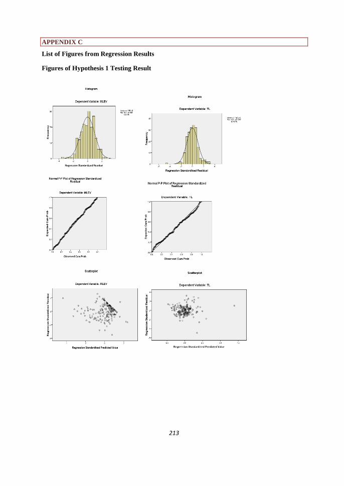
213
APPENDIX C
List of Figures from Regression Results
Figures of Hypothesis 1 Testing Result
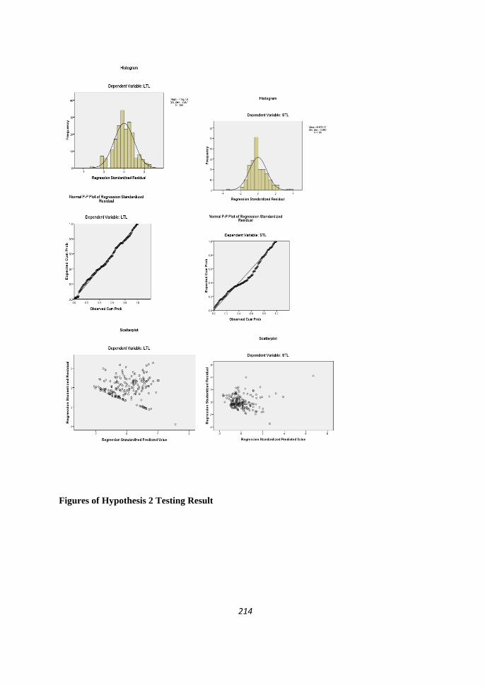
214
Figures of Hypothesis 2 Testing Result
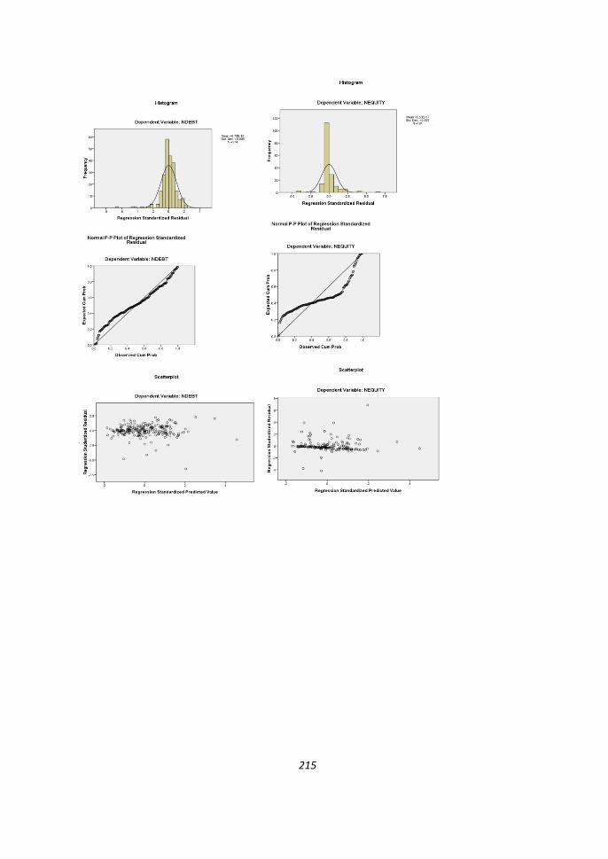
215
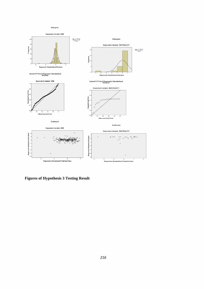
216
Figures of Hypothesis 3 Testing Result
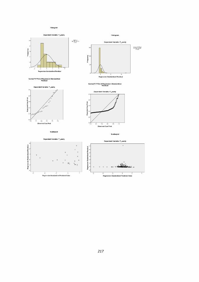
217
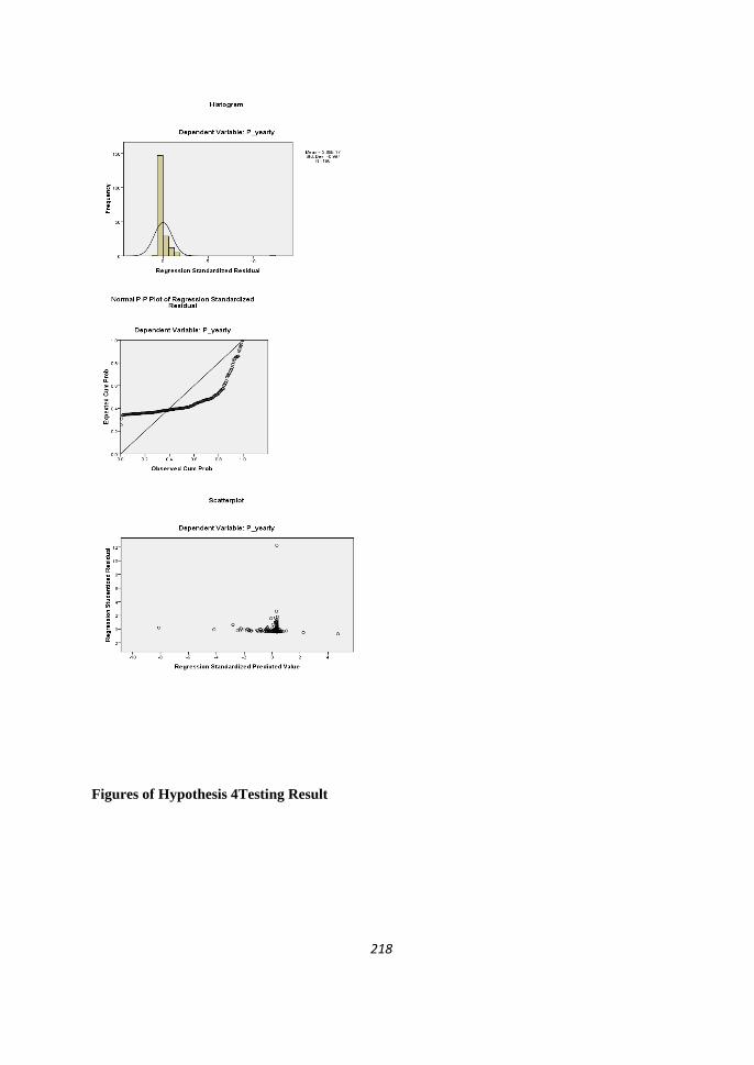
218
Figures of Hypothesis 4Testing Result
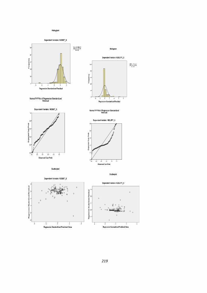
219
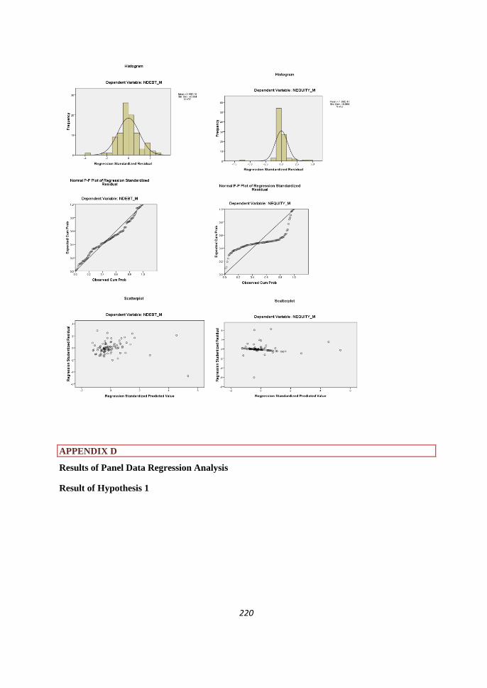
220
APPENDIX D
Results of Panel Data Regression Analysis
Result of Hypothesis 1

221
Warning: convergence not achieved; estimates are based on iterated EMNote: LR test is conservative and provided only for reference.
LR test vs. linear regression: chi2(5) = 34.15 Prob > chi2 = 0.0000 sd(Residual) .0356326 . . . sd(GROW) .1207096 . . . sd(RISK) .9367825 . . . sd(SIZE) .0060267 . . . sd(TANG) .2134466 . . . sd(PRFT) .4176825 . . .STL: Independent Random-effects Parameters Estimate Std. Err. [95% Conf. Interval]
_cons .1059268 .1282458 0.83 0.409 -.1454303 .3572839 GROW .1187629 .0435091 2.73 0.006 .0334865 .2040392 RISK .7094852 .281901 2.52 0.012 .1569695 1.262001 SIZE .0142148 .0094468 1.50 0.132 -.0043007 .0327303 TANG -.2436425 .0750988 -3.24 0.001 -.3908334 -.0964515 PRFT -.3022391 .1162004 -2.60 0.009 -.5299878 -.0744904 STL Coef. Std. Err. z P>|z| [95% Conf. Interval]
Log restricted-likelihood = 26.566101 Prob > chi2 = 0.0000 Wald chi2(5) = 40.82
max = 2 avg = 1.0 Obs per group: min = 1
Group variable: STL Number of groups = 195Mixed-effects REML regression Number of obs = 196
Hessian has become unstable or asymmetricflat or discontinuous region encounterednumerical derivatives are approximateIteration 8: log restricted-likelihood = 29.333856 (not concave)Iteration 7: log restricted-likelihood = 29.327564 (not concave)Iteration 6: log restricted-likelihood = 29.323711 (not concave)Iteration 5: log restricted-likelihood = 29.319962 (not concave)Iteration 4: log restricted-likelihood = 29.311165 (not concave)Iteration 3: log restricted-likelihood = 29.283631 (not concave)Iteration 2: log restricted-likelihood = 29.150288 (not concave)Iteration 1: log restricted-likelihood = 28.718764 Iteration 0: log restricted-likelihood = 26.566101
Performing gradient-based optimization:
Performing EM optimization:
> near. xtmixed STL PRFT TANG SIZE RISK GROW, || STL: PRFT TANG SIZE RISK GROW, noconstant covariance(independent) colli

222
Warning: convergence not achieved; estimates are based on iterated EMNote: LR test is conservative and provided only for reference.
LR test vs. linear regression: chi2(5) = 89.72 Prob > chi2 = 0.0000 sd(Residual) .0268583 . . . sd(GROW) .1150654 . . . sd(RISK) .6095126 . . . sd(SIZE) .0048396 . . . sd(TANG) .2169043 . . . sd(PRFT) .2605002 . . .LTL: Independent Random-effects Parameters Estimate Std. Err. [95% Conf. Interval]
_cons .0344509 .0505651 0.68 0.496 -.064655 .1335567 GROW .1835823 .0351526 5.22 0.000 .1146845 .2524801 RISK -.0285189 .2173788 -0.13 0.896 -.4545735 .3975357 SIZE -.0016283 .0043934 -0.37 0.711 -.0102392 .0069826 TANG .3714454 .0607135 6.12 0.000 .2524491 .4904417 PRFT -.2743938 .0857723 -3.20 0.001 -.4425045 -.1062831 LTL Coef. Std. Err. z P>|z| [95% Conf. Interval]
Log restricted-likelihood = 74.323102 Prob > chi2 = 0.0000 Wald chi2(5) = 127.64
max = 14 avg = 1.1 Obs per group: min = 1
Group variable: LTL Number of groups = 180Mixed-effects REML regression Number of obs = 196
Hessian has become unstable or asymmetricnearby values are missingnumerical derivatives are approximateIteration 2: log restricted-likelihood = 80.472139 Iteration 1: log restricted-likelihood = 78.338489 (not concave)Iteration 0: log restricted-likelihood = 74.323102
Performing gradient-based optimization:
Performing EM optimization:
> near. xtmixed LTL PRFT TANG SIZE RISK GROW, || LTL: PRFT TANG SIZE RISK GROW, noconstant covariance(independent) colli
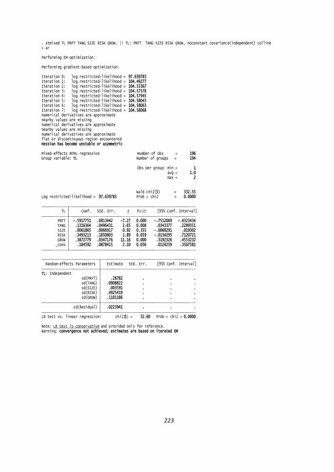
223
Warning: convergence not achieved; estimates are based on iterated EMNote: LR test is conservative and provided only for reference.
LR test vs. linear regression: chi2(5) = 32.60 Prob > chi2 = 0.0000 sd(Residual) .0223941 . . . sd(GROW) .1181186 . . . sd(RISK) .4925419 . . . sd(SIZE) .003591 . . . sd(TANG) .0908822 . . . sd(PRFT) .28782 . . .TL: Independent Random-effects Parameters Estimate Std. Err. [95% Conf. Interval]
_cons .184592 .0878415 2.10 0.036 .0124259 .3567581 GROW .3872779 .0347176 11.16 0.000 .3192326 .4553232 RISK .3493213 .1850803 1.89 0.059 -.0134295 .7120721 SIZE .0061865 .0066917 0.92 0.355 -.0069291 .019302 TANG .1316364 .0496431 2.65 0.008 .0343377 .2289351 PRFT -.5917751 .0813442 -7.27 0.000 -.7512069 -.4323434 TL Coef. Std. Err. z P>|z| [95% Conf. Interval]
Log restricted-likelihood = 97.639783 Prob > chi2 = 0.0000 Wald chi2(5) = 332.55
max = 2 avg = 1.0 Obs per group: min = 1
Group variable: TL Number of groups = 194Mixed-effects REML regression Number of obs = 196
Hessian has become unstable or asymmetricflat or discontinuous region encounterednumerical derivatives are approximatenearby values are missingnumerical derivatives are approximatenearby values are missingnumerical derivatives are approximateIteration 7: log restricted-likelihood = 104.58068 Iteration 6: log restricted-likelihood = 104.58063 Iteration 5: log restricted-likelihood = 104.58043 Iteration 4: log restricted-likelihood = 104.57945 Iteration 3: log restricted-likelihood = 104.57578 Iteration 2: log restricted-likelihood = 104.55367 Iteration 1: log restricted-likelihood = 104.49277 Iteration 0: log restricted-likelihood = 97.639783
Performing gradient-based optimization:
Performing EM optimization:
> ar. xtmixed TL PRFT TANG SIZE RISK GROW, || TL: PRFT TANG SIZE RISK GROW, noconstant covariance(independent) colline
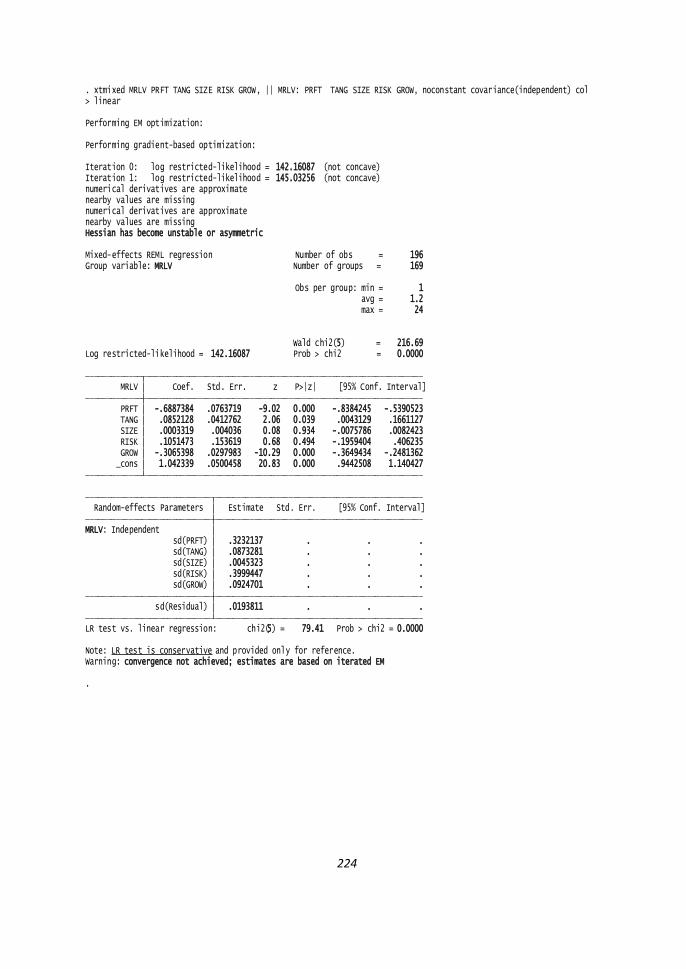
224
.
Warning: convergence not achieved; estimates are based on iterated EMNote: LR test is conservative and provided only for reference.
LR test vs. linear regression: chi2(5) = 79.41 Prob > chi2 = 0.0000 sd(Residual) .0193811 . . . sd(GROW) .0924701 . . . sd(RISK) .3999447 . . . sd(SIZE) .0045323 . . . sd(TANG) .0873281 . . . sd(PRFT) .3232137 . . .MRLV: Independent Random-effects Parameters Estimate Std. Err. [95% Conf. Interval]
_cons 1.042339 .0500458 20.83 0.000 .9442508 1.140427 GROW -.3065398 .0297983 -10.29 0.000 -.3649434 -.2481362 RISK .1051473 .153619 0.68 0.494 -.1959404 .406235 SIZE .0003319 .004036 0.08 0.934 -.0075786 .0082423 TANG .0852128 .0412762 2.06 0.039 .0043129 .1661127 PRFT -.6887384 .0763719 -9.02 0.000 -.8384245 -.5390523 MRLV Coef. Std. Err. z P>|z| [95% Conf. Interval]
Log restricted-likelihood = 142.16087 Prob > chi2 = 0.0000 Wald chi2(5) = 216.69
max = 24 avg = 1.2 Obs per group: min = 1
Group variable: MRLV Number of groups = 169Mixed-effects REML regression Number of obs = 196
Hessian has become unstable or asymmetricnearby values are missingnumerical derivatives are approximatenearby values are missingnumerical derivatives are approximateIteration 1: log restricted-likelihood = 145.03256 (not concave)Iteration 0: log restricted-likelihood = 142.16087 (not concave)
Performing gradient-based optimization:
Performing EM optimization:
> linear. xtmixed MRLV PRFT TANG SIZE RISK GROW, || MRLV: PRFT TANG SIZE RISK GROW, noconstant covariance(independent) col

225
Result of Hypothesis 2
Warning: convergence not achieved; estimates are based on iterated EM
LR test vs. linear regression: chibar2(01) = 0.00 Prob >= chibar2 = 1.0000 sd(Residual) .0525549 . . . sd(FD) .1291078 . . .NDEBT: Identity Random-effects Parameters Estimate Std. Err. [95% Conf. Interval]
_cons .0217334 .0194652 1.12 0.264 -.0164178 .0598845 FD .2377811 .0430574 5.52 0.000 .1533902 .322172 NDEBT Coef. Std. Err. z P>|z| [95% Conf. Interval]
Log restricted-likelihood = 49.945592 Prob > chi2 = 0.0000 Wald chi2(1) = 30.50
max = 2 avg = 1.0 Obs per group: min = 1
Group variable: NDEBT Number of groups = 52Mixed-effects REML regression Number of obs = 53
missing values encounteredcould not calculate numerical derivativesIteration 3: log restricted-likelihood = 50.64306 flat or discontinuous region encounterednumerical derivatives are approximateIteration 2: log restricted-likelihood = 50.64306 flat or discontinuous region encounterednumerical derivatives are approximateIteration 1: log restricted-likelihood = 50.64306 flat or discontinuous region encounterednumerical derivatives are approximateIteration 0: log restricted-likelihood = 49.945592
Performing gradient-based optimization:
Performing EM optimization:
Note: single-variable random-effects specification; covariance structure set to identity. xtmixed NDEBT FD, || NDEBT: FD, noconstant covariance(independent) collinear

226
LR test vs. linear regression: chibar2(01) = 1138.23 Prob >= chibar2 = 0.0000 sd(Residual) 1.6e-116 . . . sd(FD) .2502 .0247735 .2060658 .3037867NEQUITY: Identity Random-effects Parameters Estimate Std. Err. [95% Conf. Interval]
_cons -8.8e-215 1.3e-116 -0.00 1.000 -2.6e-116 2.6e-116 FD (dropped) NEQUITY Coef. Std. Err. z P>|z| [95% Conf. Interval]
Log restricted-likelihood = 602.34541 Prob > chi2 = . Wald chi2(0) = .
max = 5 avg = 1.1 Obs per group: min = 1
Group variable: NEQUITY Number of groups = 49Mixed-effects REML regression Number of obs = 53
Computing standard errors:
Iteration 2: log restricted-likelihood = 602.34541 (not concave)Iteration 1: log restricted-likelihood = 602.34541 Iteration 0: log restricted-likelihood = 46.0107
Performing gradient-based optimization:
Performing EM optimization:
Note: single-variable random-effects specification; covariance structure set to identity. xtmixed NEQUITY FD, || NEQUITY: FD, noconstant covariance(independent) collinear

227
Warning: convergence not achieved; estimates are based on iterated EM
LR test vs. linear regression: chibar2(01) = 0.00 Prob >= chibar2 = 1.0000 sd(Residual) .0514687 . . . sd(FD) .0441781 . . .NRE: Identity Random-effects Parameters Estimate Std. Err. [95% Conf. Interval]
_cons .0988427 .0152893 6.46 0.000 .0688762 .1288093 FD -.062957 .027202 -2.31 0.021 -.1162719 -.0096421 NRE Coef. Std. Err. z P>|z| [95% Conf. Interval]
Log restricted-likelihood = 70.209966 Prob > chi2 = 0.0206 Wald chi2(1) = 5.36
max = 1 avg = 1.0 Obs per group: min = 1
Group variable: NRE Number of groups = 53Mixed-effects REML regression Number of obs = 53
missing values encounteredcould not calculate numerical derivativesIteration 6: log restricted-likelihood = 71.826867 flat or discontinuous region encounterednumerical derivatives are approximateIteration 5: log restricted-likelihood = 71.826867 flat or discontinuous region encounterednumerical derivatives are approximateIteration 4: log restricted-likelihood = 71.826867 flat or discontinuous region encounterednumerical derivatives are approximateIteration 3: log restricted-likelihood = 71.826867 flat or discontinuous region encounterednumerical derivatives are approximateIteration 2: log restricted-likelihood = 71.826867 flat or discontinuous region encounterednumerical derivatives are approximateIteration 1: log restricted-likelihood = 71.826867 flat or discontinuous region encounterednumerical derivatives are approximateIteration 0: log restricted-likelihood = 70.209966
Performing gradient-based optimization:
Performing EM optimization:
Note: single-variable random-effects specification; covariance structure set to identity. xtmixed NRE FD, || NRE: FD, noconstant covariance(independent) collinear

228
Note: LR test is conservative and provided only for reference.
LR test vs. linear regression: chi2(2) = 1.38 Prob > chi2 = 0.5009 sd(Residual) .0648553 .0178199 .03785 .1111284 sd(FD) .0989246 .0452294 .0403762 .2423724 sd(FDSQR) .0000439 .0322742 0 .NDEBT: Independent Random-effects Parameters Estimate Std. Err. [95% Conf. Interval]
_cons .0306117 .0269366 1.14 0.256 -.0221831 .0834065 FD .1784661 .0890874 2.00 0.045 .003858 .3530743 FDSQR .0639377 .0679679 0.94 0.347 -.0692769 .1971522 NDEBT Coef. Std. Err. z P>|z| [95% Conf. Interval]
Log restricted-likelihood = 49.139212 Prob > chi2 = 0.0000 Wald chi2(2) = 36.57
max = 2 avg = 1.0 Obs per group: min = 1
Group variable: NDEBT Number of groups = 52Mixed-effects REML regression Number of obs = 53
Computing standard errors:
Iteration 10: log restricted-likelihood = 49.139212 Iteration 9: log restricted-likelihood = 49.13921 Iteration 8: log restricted-likelihood = 49.139204 Iteration 7: log restricted-likelihood = 49.139179 Iteration 6: log restricted-likelihood = 49.139023 Iteration 5: log restricted-likelihood = 49.138334 Iteration 4: log restricted-likelihood = 49.135126 Iteration 3: log restricted-likelihood = 49.123212 Iteration 2: log restricted-likelihood = 49.047105 Iteration 1: log restricted-likelihood = 48.941722 Iteration 0: log restricted-likelihood = 47.499627
Performing gradient-based optimization:
Performing EM optimization:
. xtmixed NDEBT FDSQR FD, || NDEBT: FDSQR FD, noconstant covariance(independent) collinear

229
LR test vs. linear regression: chibar2(01) = 26.87 Prob >= chibar2 = 0.0000 sd(Residual) .0005239 .0002134 .0002358 .001164 sd(FD) .0916837 .0141489 .0677536 .1240657REPOEQUITY: Identity Random-effects Parameters Estimate Std. Err. [95% Conf. Interval]
_cons -.0002445 .0003409 -0.72 0.473 -.0009126 .0004235 FD -.0415067 .0195653 -2.12 0.034 -.0798541 -.0031594 REPOEQUITY Coef. Std. Err. z P>|z| [95% Conf. Interval]
Log restricted-likelihood = 46.674918 Prob > chi2 = 0.0339 Wald chi2(1) = 4.50
max = 4 avg = 1.2 Obs per group: min = 1
Group variable: REPOEQUITY Number of groups = 22Mixed-effects REML regression Number of obs = 26
Computing standard errors:
Iteration 4: log restricted-likelihood = 46.674918 Iteration 3: log restricted-likelihood = 46.674918 Iteration 2: log restricted-likelihood = 46.674867 Iteration 1: log restricted-likelihood = 46.655047 Iteration 0: log restricted-likelihood = 40.549694
Performing gradient-based optimization:
Performing EM optimization:
Note: single-variable random-effects specification; covariance structure set to identity. xtmixed REPOEQUITY FD, || REPOEQUITY: FD, noconstant covariance(independent) collinear

230
Result of Hypothesis 3
Warning: convergence not achieved; estimates are based on iterated EM
LR test vs. linear regression: chibar2(01) = 0.00 Prob >= chibar2 = 1.0000 sd(Residual) 8761.69 . . . sd(NDEBT) 22661.17 . . .STCKPRICE: Identity Random-effects Parameters Estimate Std. Err. [95% Conf. Interval]
_cons 3711.952 726.2874 5.11 0.000 2288.455 5135.449 NDEBT 2565.906 4151.617 0.62 0.537 -5571.114 10702.93 STCKPRICE Coef. Std. Err. z P>|z| [95% Conf. Interval]
Log restricted-likelihood = -2064.4246 Prob > chi2 = 0.5365 Wald chi2(1) = 0.38
max = 4 avg = 1.3 Obs per group: min = 1
Group variable: STCKPRICE Number of groups = 146Mixed-effects REML regression Number of obs = 196
missing values encounteredcould not calculate numerical derivativesIteration 2: log restricted-likelihood = -2048.2052 flat or discontinuous region encounterednumerical derivatives are approximateIteration 1: log restricted-likelihood = -2048.2052 flat or discontinuous region encounterednumerical derivatives are approximateIteration 0: log restricted-likelihood = -2064.4246
Performing gradient-based optimization:
Performing EM optimization:
Note: single-variable random-effects specification; covariance structure set to identity. xtmixed STCKPRICE NDEBT, || STCKPRICE: NDEBT, noconstant covariance(independent) collinear

231
.
Warning: convergence not achieved; estimates are based on iterated EM
LR test vs. linear regression: chibar2(01) = 0.00 Prob >= chibar2 = 1.0000 sd(Residual) 9070.635 . . . sd(NEQUITY) 26337.34 . . .STCKPRICE: Identity Random-effects Parameters Estimate Std. Err. [95% Conf. Interval]
_cons 4017.316 713.2208 5.63 0.000 2619.429 5415.203 NEQUITY -7757.124 7958.142 -0.97 0.330 -23354.8 7840.548 STCKPRICE Coef. Std. Err. z P>|z| [95% Conf. Interval]
Log restricted-likelihood = -2054.8936 Prob > chi2 = 0.3297 Wald chi2(1) = 0.95
max = 4 avg = 1.3 Obs per group: min = 1
Group variable: STCKPRICE Number of groups = 146Mixed-effects REML regression Number of obs = 196
missing values encounteredcould not calculate numerical derivativesIteration 3: log restricted-likelihood = -2047.1948 flat or discontinuous region encounterednumerical derivatives are approximateIteration 2: log restricted-likelihood = -2047.1948 flat or discontinuous region encounterednumerical derivatives are approximateIteration 1: log restricted-likelihood = -2047.1948 flat or discontinuous region encounterednumerical derivatives are approximateIteration 0: log restricted-likelihood = -2054.8936
Performing gradient-based optimization:
Performing EM optimization:
Note: single-variable random-effects specification; covariance structure set to identity. xtmixed STCKPRICE NEQUITY, || STCKPRICE: NEQUITY, noconstant covariance(independent) collinear

232
Warning: convergence not achieved; estimates are based on iterated EM
LR test vs. linear regression: chibar2(01) = 0.00 Prob >= chibar2 = 1.0000 sd(Residual) 5697.896 . . . sd(REPOEQ~Y) 90214.21 . . .STCKPRICE: Identity Random-effects Parameters Estimate Std. Err. [95% Conf. Interval]
_cons 5235.905 1377.997 3.80 0.000 2535.08 7936.73 REPOEQUITY 57057.42 62830.01 0.91 0.364 -66087.13 180202 STCKPRICE Coef. Std. Err. z P>|z| [95% Conf. Interval]
Log restricted-likelihood = -213.03597 Prob > chi2 = 0.3638 Wald chi2(1) = 0.82
max = 1 avg = 1.0 Obs per group: min = 1
Group variable: STCKPRICE Number of groups = 23Mixed-effects REML regression Number of obs = 23
missing values encounteredcould not calculate numerical derivativesIteration 3: log restricted-likelihood = -211.95536 nearby values are missingnumerical derivatives are approximateIteration 2: log restricted-likelihood = -211.95536 flat or discontinuous region encounterednumerical derivatives are approximateIteration 1: log restricted-likelihood = -211.95536 Iteration 0: log restricted-likelihood = -213.03597
Performing gradient-based optimization:
Performing EM optimization:
Note: single-variable random-effects specification; covariance structure set to identity. xtmixed STCKPRICE REPOEQUITY, || STCKPRICE: REPOEQUITY, noconstant covariance(independent) collinear

233
Result of Hypothesis 4-Mature Firms
LR test vs. linear regression: chibar2(01) = 29.28 Prob >= chibar2 = 0.0000 sd(Residual) .1052617 .0120024 .0841808 .1316218 sd(FD_M) .1908582 .0482506 .116284 .3132577NDEBT_M: Identity Random-effects Parameters Estimate Std. Err. [95% Conf. Interval]
_cons -.0166008 .0200766 -0.83 0.408 -.0559502 .0227487 FD_M .3225679 .0640241 5.04 0.000 .197083 .4480528 NDEBT_M Coef. Std. Err. z P>|z| [95% Conf. Interval]
Log restricted-likelihood = 40.962361 Prob > chi2 = 0.0000 Wald chi2(1) = 25.38
max = 1 avg = 1.0 Obs per group: min = 1
Group variable: NDEBT_M Number of groups = 71Mixed-effects REML regression Number of obs = 71
Computing standard errors:
Iteration 3: log restricted-likelihood = 40.962361 Iteration 2: log restricted-likelihood = 40.962361 Iteration 1: log restricted-likelihood = 40.960056 Iteration 0: log restricted-likelihood = 40.648661
Performing gradient-based optimization:
Performing EM optimization:
Note: single-variable random-effects specification; covariance structure set to identity. xtmixed NDEBT_M FD_M, || NDEBT_M: FD_M, noconstant covariance(independent) collinear

234
LR test vs. linear regression: chibar2(01) = 0.01 Prob >= chibar2 = 0.4578 sd(Residual) .0960272 .008422 .0808613 .1140376 sd(FD_M) .0124699 .0616314 7.74e-07 200.8429NEQUITY_M: Identity Random-effects Parameters Estimate Std. Err. [95% Conf. Interval]
_cons -.0065849 .0144804 -0.45 0.649 -.0349658 .0217961 FD_M .0551153 .0257855 2.14 0.033 .0045767 .1056539 NEQUITY_M Coef. Std. Err. z P>|z| [95% Conf. Interval]
Log restricted-likelihood = 60.136437 Prob > chi2 = 0.0326 Wald chi2(1) = 4.57
max = 22 avg = 1.4 Obs per group: min = 1
Group variable: NEQUITY_M Number of groups = 49Mixed-effects REML regression Number of obs = 71
Computing standard errors:
Iteration 4: log restricted-likelihood = 60.136437 Iteration 3: log restricted-likelihood = 60.136437 Iteration 2: log restricted-likelihood = 60.136413 Iteration 1: log restricted-likelihood = 60.134653 Iteration 0: log restricted-likelihood = 56.764696
Performing gradient-based optimization:
Performing EM optimization:
Note: single-variable random-effects specification; covariance structure set to identity. xtmixed NEQUITY_M FD_M, || NEQUITY_M: FD_M, noconstant covariance(independent) collinear

235
Warning: convergence not achieved; estimates are based on iterated EM
LR test vs. linear regression: chibar2(01) = 0.00 Prob >= chibar2 = 1.0000 sd(Residual) .097344 . . . sd(FD_M) .1150813 . . .NRE_M: Identity Random-effects Parameters Estimate Std. Err. [95% Conf. Interval]
_cons .0921292 .0173153 5.32 0.000 .0581919 .1260666 FD_M -.0970227 .0480552 -2.02 0.043 -.1912091 -.0028363 NRE_M Coef. Std. Err. z P>|z| [95% Conf. Interval]
Log restricted-likelihood = 52.056684 Prob > chi2 = 0.0435 Wald chi2(1) = 4.08
max = 2 avg = 1.0 Obs per group: min = 1
Group variable: NRE_M Number of groups = 70Mixed-effects REML regression Number of obs = 71
missing values encounteredcould not calculate numerical derivativesIteration 4: log restricted-likelihood = 54.786413 flat or discontinuous region encounterednumerical derivatives are approximateIteration 3: log restricted-likelihood = 54.786413 flat or discontinuous region encounterednumerical derivatives are approximateIteration 2: log restricted-likelihood = 54.786413 flat or discontinuous region encounterednumerical derivatives are approximateIteration 1: log restricted-likelihood = 54.786413 flat or discontinuous region encounterednumerical derivatives are approximateIteration 0: log restricted-likelihood = 52.056684
Performing gradient-based optimization:
Performing EM optimization:
Note: single-variable random-effects specification; covariance structure set to identity. xtmixed NRE_M FD_M, || NRE_M: FD_M, noconstant covariance(independent) collinear

236
.
Note: LR test is conservative and provided only for reference.
LR test vs. linear regression: chi2(2) = 15.55 Prob > chi2 = 0.0004 sd(Residual) .1151912 .0106356 .0961231 .1380419 sd(FD_M) .0001066 .0772917 0 . sd(FDSQR_M) .1107299 .0542753 .0423682 .289394NDEBT_M: Independent Random-effects Parameters Estimate Std. Err. [95% Conf. Interval]
_cons -.0341197 .0236224 -1.44 0.149 -.0804187 .0121793 FD_M .4545407 .1046305 4.34 0.000 .2494686 .6596127 FDSQR_M -.0865629 .0911667 -0.95 0.342 -.2652464 .0921205 NDEBT_M Coef. Std. Err. z P>|z| [95% Conf. Interval]
Log restricted-likelihood = 41.421959 Prob > chi2 = 0.0000 Wald chi2(2) = 39.84
max = 1 avg = 1.0 Obs per group: min = 1
Group variable: NDEBT_M Number of groups = 71Mixed-effects REML regression Number of obs = 71
Computing standard errors:
Iteration 10: log restricted-likelihood = 41.421959 Iteration 9: log restricted-likelihood = 41.421958 Iteration 8: log restricted-likelihood = 41.421947 Iteration 7: log restricted-likelihood = 41.421882 Iteration 6: log restricted-likelihood = 41.421585 Iteration 5: log restricted-likelihood = 41.420292 Iteration 4: log restricted-likelihood = 41.415146 Iteration 3: log restricted-likelihood = 41.398807 Iteration 2: log restricted-likelihood = 41.259676 Iteration 1: log restricted-likelihood = 41.169184 (not concave)Iteration 0: log restricted-likelihood = 38.445682
Performing gradient-based optimization:
Performing EM optimization:
. xtmixed NDEBT_M FDSQR_M FD_M, || NDEBT_M: FDSQR_M FD_M, noconstant covariance(independent) collinear

237
Result of Hypothesis 4-Growth Firms
LR test vs. linear regression: chibar2(01) = 37.69 Prob >= chibar2 = 0.0000 sd(Residual) .1804201 .0160204 .151601 .2147175 sd(FD_G) .2548314 .0341446 .1959754 .3313634NDEBT_G: Identity Random-effects Parameters Estimate Std. Err. [95% Conf. Interval]
_cons -.0918211 .0281735 -3.26 0.001 -.1470402 -.036602 FD_G .3107493 .0531525 5.85 0.000 .2065724 .4149263 NDEBT_G Coef. Std. Err. z P>|z| [95% Conf. Interval]
Log restricted-likelihood = 1.0795205 Prob > chi2 = 0.0000 Wald chi2(1) = 34.18
max = 2 avg = 1.0 Obs per group: min = 1
Group variable: NDEBT_G Number of groups = 152Mixed-effects REML regression Number of obs = 153
Computing standard errors:
Iteration 4: log restricted-likelihood = 1.0795205 Iteration 3: log restricted-likelihood = 1.0795205 Iteration 2: log restricted-likelihood = 1.0795059 Iteration 1: log restricted-likelihood = 1.0781159 Iteration 0: log restricted-likelihood = .83363296 (not concave)
Performing gradient-based optimization:
Performing EM optimization:
Note: single-variable random-effects specification; covariance structure set to identity. xtmixed NDEBT_G FD_G, || NDEBT_G: FD_G, noconstant covariance(independent) collinear

238
LR test vs. linear regression: chibar2(01) = 55.25 Prob >= chibar2 = 0.0000 sd(Residual) .0911003 .0084938 .0758853 .1093659 sd(FD_G) .1949145 .024343 .1525938 .2489726NEQUITY_G: Identity Random-effects Parameters Estimate Std. Err. [95% Conf. Interval]
_cons .0143126 .0145739 0.98 0.326 -.0142518 .042877 FD_G .0762942 .0327744 2.33 0.020 .0120576 .1405308 NEQUITY_G Coef. Std. Err. z P>|z| [95% Conf. Interval]
Log restricted-likelihood = 89.238384 Prob > chi2 = 0.0199 Wald chi2(1) = 5.42
max = 42 avg = 1.4 Obs per group: min = 1
Group variable: NEQUITY_G Number of groups = 109Mixed-effects REML regression Number of obs = 153
Computing standard errors:
Iteration 2: log restricted-likelihood = 89.238384 Iteration 1: log restricted-likelihood = 89.238383 Iteration 0: log restricted-likelihood = 89.232193
Performing gradient-based optimization:
Performing EM optimization:
Note: single-variable random-effects specification; covariance structure set to identity. xtmixed NEQUITY_G FD_G, || NEQUITY_G: FD_G, noconstant covariance(independent) collinear

239
LR test vs. linear regression: chibar2(01) = 38.91 Prob >= chibar2 = 0.0000 sd(Residual) .0888251 .0065607 .0768538 .1026611 sd(FD_G) .0961413 .0133906 .0731736 .126318NRE_G: Identity Random-effects Parameters Estimate Std. Err. [95% Conf. Interval]
_cons .0501018 .0133079 3.76 0.000 .0240188 .0761849 FD_G -.0673261 .0237537 -2.83 0.005 -.1138825 -.0207696 NRE_G Coef. Std. Err. z P>|z| [95% Conf. Interval]
Log restricted-likelihood = 120.65754 Prob > chi2 = 0.0046 Wald chi2(1) = 8.03
max = 2 avg = 1.0 Obs per group: min = 1
Group variable: NRE_G Number of groups = 150Mixed-effects REML regression Number of obs = 153
Computing standard errors:
Iteration 3: log restricted-likelihood = 120.65754 Iteration 2: log restricted-likelihood = 120.65754 Iteration 1: log restricted-likelihood = 120.65744 Iteration 0: log restricted-likelihood = 120.43421
Performing gradient-based optimization:
Performing EM optimization:
Note: single-variable random-effects specification; covariance structure set to identity. xtmixed NRE_G FD_G, || NRE_G: FD_G, noconstant covariance(independent) collinear

240
Note: LR test is conservative and provided only for reference.
LR test vs. linear regression: chi2(2) = 47.27 Prob > chi2 = 0.0000 sd(Residual) .1852066 .0125883 .1621069 .2115981 sd(FD_G) .0000683 .0490102 0 . sd(FDSQR_G) .1997736 .0346679 .1421752 .2807064NDEBT_G: Independent Random-effects Parameters Estimate Std. Err. [95% Conf. Interval]
_cons -.1152962 .0270128 -4.27 0.000 -.1682403 -.0623521 FD_G .6283551 .0777452 8.08 0.000 .4759773 .780733 FDSQR_G -.3936119 .0843204 -4.67 0.000 -.5588769 -.2283469 NDEBT_G Coef. Std. Err. z P>|z| [95% Conf. Interval]
Log restricted-likelihood = 15.667864 Prob > chi2 = 0.0000 Wald chi2(2) = 71.90
max = 2 avg = 1.0 Obs per group: min = 1
Group variable: NDEBT_G Number of groups = 152Mixed-effects REML regression Number of obs = 153
Computing standard errors:
Iteration 12: log restricted-likelihood = 15.667864 Iteration 11: log restricted-likelihood = 15.667863 Iteration 10: log restricted-likelihood = 15.667856 Iteration 9: log restricted-likelihood = 15.667824 Iteration 8: log restricted-likelihood = 15.667694 Iteration 7: log restricted-likelihood = 15.667111 Iteration 6: log restricted-likelihood = 15.664364 Iteration 5: log restricted-likelihood = 15.651562 Iteration 4: log restricted-likelihood = 15.602732 Iteration 3: log restricted-likelihood = 15.389318 Iteration 2: log restricted-likelihood = 14.629784 Iteration 1: log restricted-likelihood = 11.295448 (not concave)Iteration 0: log restricted-likelihood = 8.620027 (not concave)
Performing gradient-based optimization:
Performing EM optimization:
. xtmixed NDEBT_G FDSQR_G FD_G, || NDEBT_G: FDSQR_G FD_G, noconstant covariance(independent) collinear

241
APPENDIX E
CV
1. PERSONAL
Siti Rahmi Utami
Born Jakarta, September 13, 1976
2. EDUCATION Master of Philosophy (MPhil), 2005-2008, Maastricht School
of Management (Netherlands).
Master of Management (MM), 2001-2003, University of
Trisakti (Indonesia).
Bachelor Degree (ST) in Environmental Engineering, 1995-
2000, University of Trisakti (Indonesia).
3. PUBLICATIONS
International Journal The Pecking Order Theory : Evidence from Manufacturing
Firms in Indonesia (with Prof. Eno L. Inanga), published by
Independent Business Review, Issue 1, No.1, (2008).
Foreign Exchange Rates, Interest Rates, and Inflation Rates in
Indonesia the International Fisher Effect Theory (with Prof.
Eno L. Inanga), published by International Research Journal of
Finance and Economics, Issue 26 (April 2009), pp.151-169.
Agency Costs of Free Cash Flow, Dividend Policy, and
Leverage of Firms in Indonesia (with Prof. Eno L. Inanga),
published by European Journal of Economics, Finance and
Administrative Sciences, Issue 33 (2011), pp.1-18.
Significance of Accounting Information in Explaining Market
and Book Values: The Case of Indonesian Banks (with Noraya
Soewarno, Siti Rahmi Utami as co-Author), published by
International Research Journal of Finance and Economics,
Issue 55 (2010), pp.146-157.

242
Indonesian Journal Efficient Market Hypothesis : Evidence from Indonesia Stock
Exchange (IDX), published by Ultima Accounting, University
of ultimedia Nusantara, Volume 1 (December 2009), pp.10-
17.
Seminar Paper Analisis January Effect pada Indeks LQ45, presented in
National Seminar at University of Atmajaya, Indonesia, 25-
26th
of May 2010.
4. ACCEPTED ARTICLE FOR PUBLICATION
Titled The Relationship between Capital Structure and the Life
Cycle of Firms in the Manufacturing Sector of Indonesia (with
Prof. Eno L. Inanga), will be published in International Research
Journal of Finance and Economics.