Embed Size (px)
Citation preview

DTI
OF S
.1*
VALIDATION OF AN EXPONENTIALLY
DECREASING FAILURE RATE SOFTWARE
RELIABILITY MODEL
THESIS
Charles J. Westgate, ICaptain, USAF
DorJ.7loN 9TAjk7:m7?T A
Apyoved tr nL Cf w!eam0
Dis twu non Uni~rtedDTPRTMNTOF THE AIR FORCE
AIR UNIVERSITY
AIR FORCE INSTITUTE OF TECHNOLOGY
Wright-Patterson Air Force Base, Ohio
89 12 19 023

AFIT/GLM/LSY/89S-71
DTICS ELFCT F. *,
DEC 20 1900 :
VALIDATION OF AN EXPONENTIALLY
DECREASING FAILURE RATE SOFTWARE
RELIABILITY MODEL
THESIS
Charles J. Westgate, IIICaptain, USAF
AFIT/GLM/LSY/89S-71
Approved for public release; distribution unlimited

The contents of the document are technically accurate, and nosensitive items, detrimental ideas, or deleterious information iscontained therein. Furthermore, the views expressed in thedocument are those of the author and do not necessarily reflectthe views of the School of Systems and Logistics, the AirUniversity, the United States Air Force, or the Department ofDefense.
Acce;o) Fo,
0.j o" .-d J
J ) I ,bI t, "
!.ld' -b y (,odes
A.~ ,) IDist
r\-i _

AFIT/GLM/LSY/89S-71
VALIDATION OF AN EXPONENTIALLY
DECREASING FAILURE RATE
SOFTWARE RELIABILITY MODEL
THESIS
Presented to the Faculty of the School of Systems and
Logistics of the Air Force Institute of Technology
Air University
In Partial Fulfillment of the
Requirements for the Degree of
Master of Science in Logistics Management
Charles J. Westgate, III, B.S., M.S.
Captain, USAF
September 1989
Approved for public release; distribution unlimited

Preface
The purpose of this study was to determine the degree of
validity of the Air Force Operational Test and Evaluation
(AFOTEC) Software Reliability Estimation Model. The results
of my research should help AFOTEC, the Air Force and all
partieE involved in buying or developing software. My intent
in performing this research was to provide a tool that would
be easy to use and have the degree of accuracy needed to make
this model a valid tool.
In performing this research, I received assistance from
several others. Without this help, I feel this document that
you are now reading would not have been possible. First, I
wish to thank Prof. Dan Ferens for his guidance and technical
expertise. My wholehearted thanks to Lt Col Bruce Christensen
for assistance in the area of statistics and to Capt Mike
McPherson for the failure data and his knowledge of the AFOTEC
Model. I must also express my appreciation to Dr. C. R. Fenno
for his assistance in the grammar and format of this document.
Most of all, 1 wish to thank my wife Barbara and daughter Beth
for their patience and understanding throughout these last
fifteen months.
Charles J. Westgate, III
ii

Table -of Contents
Page
Preface...........................ii
List of Figures........................v
List of Tables......................vii
Abstract.........................viii
I. Introduction.......................
Overview......................1Definitions........................IBackground.....................2General Issue....................8Research Question..................9Research Objectives . ... .. .. .. .. ...... 10Justification....................10Scope and Limitations................11Summary......................11
II. Literature Review...................12
Introduction....................12Scope........................12General Model Types.....................12Current Software Reliability Models. ........ 14Fault Tolerance..................22Application and Guidance..............26Validation Methods................27Conclusions.....................29
III. Methodology......................31
Introduction....................31Model Feasibility.................31Model Validation..................32Model Assumptions.................35Summary....................... .... 36
IV. Findings and Analysis.................37
Introduction....................37Model Feasibility.................37Model Validation.................38
iii

Model Assumptions ..... ............... 45
Summary and Conclusions .... ........... 46
V. Conclusions and Recommendations .. .......... 48
Introduction ...... .. ............... 48Conclusions ....... .................. 48Recommendations ..... ................ 50Summary ........ .................... 53
Appendix A: Analysis of Model A ............ 54
Appendix B: Analysis of Model B ..... ......... 59
ATndix C: AFOTEC Paper ..... ................ 62
Appendix D: List of Acronyms and Symbols . ........ 77
Appendix E: Graphs and Data Plots ... ........... 79
Appendix F: Research Data Sets .... ............. 91
Bibliography ......... ...................... 102
VITA ........... .......................... 105
iv

List of Figures
Figure Page
I. Growth in Military Aircraft SoftwareRequirements ...... .... ................. 3
2. Growth in Software Demand for Space Systems . . 4
3. Hardware and Software Cost Trend .... ....... 5
4. Software Maintenance Cost Trend ..... ........ 6
5. Software Life Cycle Cost per Phase ... ...... 7
6. Fix Cost per Error per Phase ..... ......... 8
7. AFOTEC Model of Software Faults .. ........ 20
8. S-Shaped Software Fault Model .. ......... 20
9. Trend in Software Personnel ... .......... 25
10. Model Versus Actual for AFOTEC Model ..... 40
11. Model Versus Actual for Model A ......... 55
12. Model versus Actual for APOTEC Model(Data Set 01) .......... ................. 79
13. Model versus Actual for AFOTEC Model(Data Set 02) ....... ................. 80
14. Model versus Actual for AFOTEC Model(Data Set #3) ......... ............. 81
15. Model versus Actual for AFOTEC Model(Data Set #4) ....... ................. 82
16. Model versus Actual for APOTEC Model(Data Set #5) ....... ................. 83
17. Model versus Actual for AFOTEC Model(Data Set #6) ....... ................. 84
18. Model versus Actual for Model A(Data Set #1) ...... .... ................. 85
19. Model versus Actual for Model A(Data Set #2) ....... ................. 86
v

20. Model versus Actual for Model A(Data Set #3)...................87
21. Model versus Actual for Model A(Data Set #4)...................88
22. Model versus Actual for Model A(Data Set #5)...................89
23. Model versus Actual for Model A(Data Set #6)...................90
vi

List of Tables
Table Page
I. DOD Severity Codes ..... .............. 19
II. Parameter Intervals Analysis for the AFOTECModel ......... ..................... 41
III. Coefficient of Determination Analysis for theAPOTEC Model ....... ................. 43
IV. Residual Analysis for the APOTEC Model . . . . 44
V. Analysis of Predictions for the AFOTEC Model 45
VI. Parameter Interval Analysis for Model A .... 56
VII. Coefficient of Determination Analysis forModel A ......... .................. . 56
VIII. Residual Analysis for Model A .. ......... 57
IX. Analysis of Predictions for Model A ....... 58
vii

AFIT/GLM/LSY/89S-71Abstract
The purpose of this thesis was to determine the validity
of a software reliability estimation model proposed by the
Air Force Operational Test and Evaluation Center (AFOTEC).
During the last forty years of the computer era, the demand
for software has been growing at a rate of twelve percent per
year: and about f:lty percent of the total life cycle cost of
a software system is attributed to software maintenance. It
has also been shown that the cost of fixing a software fault
increases dramatically as the life cycle progresses. It was
statistics like those discussec above that prompted this
research.
The research had these specific objectives: the first was
ascertaining the soundness of the model's intrinsic logic.
The second objective was to run the model with actual failure
data to measure the validity and correlation of the data with
the model. The final objective was to determine the
assumptions required to operate the model.
The study found the AFOTEC Model to be invalid; however,
improvements and assumpt; ns could be easily applied to make
the model a valid tool for estimating software reliability.
Two improvements were proposed for the AFOTEC Model. First.
the model should operate with the assumption that the data
used in the model should be data obtained after softwate
viii

testing has reached a steady state. The second recommendatlon
was to modify the AFOTEC Model to emulate both the start-up
phase and the steady state phase of testing.
ix

VALIDATION OF AN EXPONENTIALLY DECREASING FAILURERATE SOFTWARE RELIABILITY MODEL
I. Introduction
Overview
This chapter discusses the evolution of military weapon
systems, and the growing role that software has in these
systems. By addressing these issues, the need for reliable
software will be revealed. The justification for the research
has also been presented, and finally, the specific objectives,
assumptions, and scope of the research has been established.
Definitions
The term reliability refers to the probability that a
system will not fail within a given amount of time, and
failure rate refers to the rate at which failures occur in a
system at a specified time (24:80-84). For the purposes of
this research, software reliability will be defined as "the
probability of failure-free operation of a computer program
for a specified time" (32:15). The software failure rate is
defined as the rate at which software bugs or faults are
discovered and is expressed as the number of failures per time
(32:15-16). Finally, the term mean time between failures
(MTBF) is the average time expected before the next fault is
detected. The MTBF can also be mathematically defined as the
inverse of the failure rate (24:80-84). The terms
reliability, mean time between failure (MTBF) and failure rate
will be used as measures of software reliability.
Background
Throughout history, men have used mechanical/hardware
weapon systems. From the first time that a prehistoric man
used a rock as a weapon, we have been using hardware systems.
However, it has been within the last 43 years that computers
and software have come into existence (20:126), and only the
last 37 years that computers have been commercially available
(30:54). Thus, there has been much more research and
knowledge in the topic of hardware and hardware reliability
than in the area of software and software reliability.
The use of computers and software is increasing rapidly,
however (26:41). For example, the first computer, the ENIAC,
was built about 40 years ago and it was only capable of
performing simple arithmetic functions at a speed of about 2.8
milliseconds (30:35). This computer weighed 30 tons (30:34)
and occupied a space 100 feet long, 10 feet high and 3 feet
deep (20:126). Today, a calculator can perform over 100
mathematical operations and can fit in the palm of a hand.
Another example. the software in the B-lB Bomber performs
up to one million calculations per second to keep the aircraft
2

flying (6:18), which is about one thousand times faster than
the ENIAC computer. An example of the growing demand for
software in military aircraft is shown in Figure 1.
4000 A E-3AAAIR FORCE
o o NAVY1000
S00 0 F-18X
0 0 P-3C
S300AD B-1 / / F-1 5 W/RADAR RSP
0 E-3A 0200 A F-16
O B-52 OASP-3C E2C UPDATE
100 C-SA A F-iS19 1FB-111-1 5
0 EF-111
1965 1970 1975 1980
Reprinted from (26:42)
Figure 1: Growth in Military AircraftSoftware Requirements
This figure illustrates how the amount of software,
measured in the number of lines of code, has increased in
United States aircraft throughout the years. A similar
example for space systems is shown in Figure 2.
3

Space40 -Shuttle
Z 0 -2 "
.0
Apollo-Skylab10
GeminiMercury
SI -A-----
1960 1965 1970 1975 190
Reprinted from (5:643)
Figure 2: Growth in Software Demandfor Space Systems
Figure 3 represents the increase in software versus
hardware in Air Force systems, measured as a percent of the
total system cost. At this rate of growth, the Air Force
cannot afford to overlook software (26:44).
Reliability has also grown in importance in the last few
years, as the Air Force's Reliability and Maintainability
Project, R & M 2000, demonstrates (10:1). By making systems
more reliable, the systems should, by definition, fail less
often; hence, less money should be spent maintaining these
systems (31:15). In light of current budget cuts and the
Graham-Rudman-Hollings Act, the Air Force has been required
4

to operate the same systems, but with a smaller budget
(31:12).
80so- Hardware
60
40
0
1955 1970 1985
Year
Reprinted from (35:11)
Figure 3: Hardware and SoftwareCost Trend
Historically, about sixty percent of the total dollars
spent on a weapon system is used for operating and maintaining
the system (4); and, as shown in Figure 4, the cost of
software maintenance is increasing as a percent of total
system cost.
According to Halpin, 20 to 25 percent of all system
failures are due to software faults (21:5.1). Glass states
that 50 percent of the software life cycle cost is spent on
software maintenance (Figure 5). Glass also claims, as showt
in Figure 6, the cost to correct a software fault "increases
dramatically as the software progresses through the life
cycle" (18:11),
5

0
Hardwre
i Oe0mlopment
- 60
40
C
20-Maneac
01955 1970 1985
Year
Reprinted from (5:18)
Figure 4: Software MaintenanceCost Trend
Since the demand for software has been shown to be rapidly
increasing along with the cost of maintaining software, money
could be saved if software was produced reliably during the
development phase. Hence, more reliable systems would help
to cut costs. The cost savings is one of the reasons that the
Air Force instituted the Reliability and Maintainability (R&M)
2000 Program (10:1).
Although the Air Force implemented R&M 2000 to cover both
hardware and software, it does not provide much guidance on
how to handle software reliability. The R&M 2000 Program Plan
provides guidance on how reliability and maintainability
6

programs should be developed and managed; however, the
document does not mention how software reliability should be
handled (25:356).
Raintenan e~(50%)
Requirements
Spifiction Checkout(10%) (20\ hk)
Design
Reprinted from (18:8)
Figure 5: Software Life CycleCost per Phase
The only guidance given by the Air Force can be found in
Air Force Regulation (APR) 800-18, which only directs:
"Integrate the development of reliable software into the
overall system development and acquisition program" (9:3).
No other information or direction is given on how to develop
reliable software or how to measure the reliability. In fact,
a military standard directs that, when calculating system
7

reliability, the software reliability should be assumed to be
completely reliable (11:100-3). Thus, it is important to
research the area of measuring the reliability of software and
the techniques of developing reliable software.
Reprinted from (18:11)
Figure 6: Fix Cost per Errorper Phase
General Issue
The general question examined in this thesis was how to
improve the reliability of the software that accounts for a
major portion of the United States Air Force's weapon systems.
The answer to this question will not only increase the
reliability of the software or computer program in these
8

weapon systems, but will also improve the reliability of the
entire system.
Research Question
In order to improve the reliability of software, a method
should first be developed to measure the reliability. This
measurement is required to determine if a technique for
improving reliability has in fact made an improvement. After
a system of measurement has been developed, proposed
reliability improvement techniques can be compared using the
measurement system. The comparisons can be used to judge
which improvement technique will, in fact, result in
improvements; and which techniques will provide the best
results. For example, a reliability model could be used to
compare various software fault tolerance techniques.
The research question that has been anSwGLed in this thesis
is how to quantitatively measure the reliability of software.
To answer this question, it was first necessary to decide if
a new model should be developed and validated to measure
software reliability or if an existing model could be chosen
to be validated. After researching the current literature on
the topic of software reliability and contacting organizations
that have ongoing research in the area, it was determined that
several models are already in existence. Hence, it was
decided to choose an existing model. Therefore, the specific
research question is: What is the validity of the software
9

reliability model that has been developed by the Air Force
Operational Test and Evaluation Center (AFOTEC) to measure the
reliability of software during the operational test and
evaluation (OT&E) phase of a development program?
Research Objectives
To determine if the AFOTEC Model is valid, three objectives
had to be met. The first objective was to ascertain if the
theory behind the model is sound and, if so, to what extent.
The second objective was to run the model with existing data
to evaluate how well it predicted reliability. The final
objective was to conclude under what assumptions the model was
valid and to comment on the applicability of the model during
othet phases of the development cycle.
Justification
Since the model chosen to be validated was developed by the
Air Force Operational Test and Evaluation Center, they have
sponsored this research realizing that the findings could help
standardize the way in which both AFOTEC and the Air Force
define and measure software reliability (22). The results of
this research can also be applied to Air Force acquisition
contracts as a method of determining the degree to which the
system under contract meets a given reliability requirement
in the specification, and to determine if the software meets
the reliability requirements of the operational commands.
10

Scope and Limitations
The scope of this research is limited to the validation of
the AFOTEC Model during the operational test and evaluation
phase; however, generalizations will be made as to the model's
validity during other phases of the acquisition cycle.
Another limitation to this research is in the use of available
data. Enough time is not available to develop software and
collect a primary source of data; therefore, the analysis has
been limited to the use of secondary or already existing
databases. This data has been obtained from Rome Air
Development Center (RADC), AFOTEC, and the Aeronautical
Systems Division (ASD) Information Center (INFOCEN).
Summary
This chapter discussed the importance of reliable software
and how it can affect the maintenance and budgetary
requirements of the Air Force. It has also been pointed out
that before developing reliable software, a method for
measuring software reliability should first be developed.
Chapter II contains a summary of the current literature and
research in the areas of software reliability, fault tolerance
and reliability improvement techniques, current Air Force
guidance, and statistical model validation techniques.
11

II. Literature Review
Introduction
This chapter is a review of literature that deals with the
topics of reliability and fault tolerance of software. It
also covers current Air Force guidance for managing software
reliability and techniques of validating statistical models.
Scope
The literature search was limited to the last fifteen years
because, according to Dunham, research in the area of software
reliability did not begin until 1972 (15:111). The search
concentrated on military applications, although it was not
confined to this area. Literature searches were performed
through the National Aeronautics and Space Administration
(NASA), Defense Technical Information Center (DTIC), DIALOG,
and RADC literary databases.
General Model Types
Currently, several types of models exist that are capable
of estimating the reliability of software or counting the
number of errors in a program. The five general types of
models are mean time between failure, error counting, error
seeding, metrics, and input domain (16:1-6). However, they
are not all useful for all stages in the software life cycle,
and they have not been proven to be valid models.
12

Error Countini Models. Error counting models or
exponentially decreasing failure rate models usually assume
a Poisson distribution for the number of errors remaining at
some point in time (16:2). This type of model is useful
during the final stages of software developzuent, such as
integration and test, acceptance test, and operational use
(19:1418-1420). Estimating the input parameters for these
models, however, can be difficult. A typical parameter which
must be estimated is the initial number of errors in the
software; however, error seeding models can estimate this
number.
Error Seeding Models. The error seeding models require a
programmer to insert faults into the software, and then an
independent programmer counts the number of errors that he or
she finds. The model uses a ratio of the number of seeded
errors detected to the number of non-seeded errors. The ratio
is used to estimate the initial number of errors in the
software (16:2). This model can be useful during the unit
test phase or when used to estimate the input parameter of
another model (19:1419).
Mean Time Between Failure Models. The mean time between
failure (MTBF) models are very similar to the error counting
models. The MTBF models calculate the estimated time until
the next error will be detected, as compared to the error
counting models tha estimate the number of errors detected
by some point in time (16:3).
13

Metrics Models. Metrics models use qualitative inputs to
a model to obtain quantitative values of the software quality.
Examples of the inputs include complexity of the software,
programming language used, experience of the programmer, and
programming structure. All of these inputs require a
subjective evaluation of parameters that are difficult to
quantify. Bruce Brocka suggests software should not be
evaluated for reliability; rather, it should be measured for
maturity and utility (8:28). The use of a Metrics model is
one such method of measuring maturity and utility.
Input Domain Models. Input domain models operatc on a
ratio principle simiJar to the fault seeding. models. Input
domain models use a set of test cases or input parameters that
are generated to represent the expected operating environment.
The reliability is assumed to be proportional to the ratio of
the number of cases that cause an error to the total numL 2r
of cases generated (19:1416).
Current Software Reliability Models
Currently, there are approximately forty models that have
been developed to estimate software reliability (1:94). The
following section contains a brief description of some of the
more popular models that have been developed to estimate
software reliability.
Schick - Wolverton Linear Model. The Schick - Wolverton
Model is an example of a time between failure model becausp
14

it calculates a failure rate based on the time between the
ith and the (i-l)st failure. This failure rate is expressed
by a Rayleigh distribution and can be expressed by:
h(t i) = K[E O - (i-l)]x i (I)
and the reliability is defined as:
R(t i) = exp[-h(ti)*t/2] (2)
where
K = constant of proportionalityEO = initial number of errors in the programx i = debugging time between the (i-l)st and ith error
The equations above assume that the time required to remove
faults is negligible and that new faults are not introduced
during debugging (14:118-124).
Jelinski - Moranda Model. This model was developed in
1972, and is another example of a time between failure model
(19:1413). The Jelinski - Moranda Model is similar in form
to the Schick - Wolverton Model; however, the failure rate is
distributed exponentially and is only proportional to the
number of faults remaining at some time. The failure rate is
defined as:
h(t i) = K[E 0 - (i - 1)] (3)
and the reliability is given by:
R(ti) - exp[-h(t.) * ti (4)
The Jelinski - Moranda Model has the same assumptions as
discussed above (14:118-123).
Shooman Model. Shooman's failure count model was also
developed in 1972, and it assumes the failure rate to be
15

proportional to the number of faults per machine language
instruction (35:369). Shooman defines the failure rate to
be:
h(t) = K[(N/I) - n] (5)
where
N = initial number of errorsI = total number of machine language instructionsn = total number of faults corrected by time, t
The two unknowns in the Shooman Model, N and K, must be
determined before this model can be used. A technique known
as moment matching can be used to provide an estimate of these
parameters. Dhillon and Singh's text provides a solution for
these parameters as well as a reference on the moment matching
technique (14:121-122).
Goel - Okumoto Nonhomogeneous Poisson Model. The Goel -
Okumoto Model represents the failure rate as exponentially
decreasing. For this model, the cumulative number of faults
detected by time, t is given by:
M(t) = all - exp(-bt)] (6)
therefore, by taking the derivative, the failure rate is
determined by differentiating equation (6):
M'(t) = ab[exp(-bt)] (7)
where
a = total expected number of software faultsb = fault detection rate per faultt = cumulative time on test
The "a" and "b" can be estimated by a maximum likelihood
function calculated using sample failure data (19:1415).
16

Musa Execution Time Model. The Musa Model was developed
in 1975 and is another example of a failure counting model.
The model assumes the failure rate to be proportional to the
number of faults remaining in the program after t units of
CPU time. The failure rate is expressed by:
h(t) = Kf(N - n) (8)
where
K = constant of proportionalityN = initial number of faults
n = number of faults corrected by time, tf = E/IE = average instruction execution rateI = number of instructions in the program
Musa's model uses the actual Computer Processing Unit (CPU)
execution time rather than the amount of time on test;
therefore, the estimated reliability should not be
artificially increased due to an increase in testing time
(32:285-288).
APOTEC Model. The following information dealing with the
AFOTEC Model is taken from an unpublished paper by Wiltse,
McPherson and Holmquist of AFOTEC titled "Predicting System
Reliability: Software and Hardware" (27:1-15). A copy or
this document can be found in Appendix C.
The purpose of the APOTEC Model is to provide a practical
method of combining hardware and software reliability data
during Operational Test and Evaluation (OT&E), in order to
estimate the system reliability. Prior to using this model,
APOTEC considered software to be 100% reliable.
17

Although AFOTEC's model was derived from the Goel - Okumoto
Failure Count Model, there are two major differences between
the two models. 'First, the AFOTEC Model uses calendar dates
(day-month-year) rather than execution or testing time. The
use of calendar time has been demonstrated by Musa (32:54-57)
to be a valid method of modeling software faults. Second,
AFOTEC added an imperfect debugging model that represents a
pessimistic bound on the reliability.
When AFOTEC is performing tests on software, they recorJ
the following information for each software fault discovered:
the date fault was discovered, a prcblem number, the affected
computer program configuration item (CPCI), a DOD severity
code (See Table I), a description of the problem, and the date
the fault --as fixed. However, the AFOTEC Software Reliability
Mcdel only uses the date the fault was discovered and the
cumulative number of faults discovered. The APOTEC Model also
limits the data to those faults with an associated DOD
severity code of 1 or 2.
AFOTEC's basic model has the same form as the Goel -
Okumoto Model shown above in equations (6) and (7). This
basic model is used to estimate the "a" and "b" parameters
from the sample failure J-ta. AFOTEC's model operates under
assumption that at the beginning ot testing, faults will be
discovered at fast rate; however, as fewer faults remain, the
slower they will be discovered. Figure 7 shows a graphical
representation of what the model expects.
18

Table I: DOD Severity Codes
Reprinted from (27:6)
SeverityLevel Severity Description
1 System Abort. A software of firmware problem thatresults in a system abort.
2 System Degraded. A software of firmware problem thatNo Work-around. severely degrades the system and no
alternative work-around exists (programrestarts not acceptable).
System Degraded. A software or firmwure problem thetWork-around. severely degrades the system and there
exists an alternative work-around(i.e. system rerouting through operatorswitchology: no program restarts).
4 Software Problem. An indicated software of firmware problemSystem not that does not severely degrade the systemDegraded. or any essential system function.
5 Minor Pault. All other minor deficiencies of non-functional faults.
Although most models assume the failure rate to be
decreasing (Figure 7), some authors do not always agree.
Yamada and Osaki believe the failure rate could exhibit an S-
shape (Figure 8), thus the failure rate initially increases
and eventually decreases (36:1433). They believe the S-shape
is due to one of two reasons. First, the process of isolating
a fault could cause the initial low failure rate. Second,
failure detection could be dependent on the number of errors
already detected; therefore, the more failures are detected,
then the more undetected failures become detected (36:1433).
19

Adapted from (27:7)
Figure 7: AFOTEC Model of Software Faults
Adapted from (36:1433)
Figure 8: S-Shaped Software
Fault Model
20

McPherson does not agree with Yamada and Osaki, and states
that the S-shaped data could be due to slow testing initially,
or due to systems with higher priorities taking test time from
the system (28).
AFOTEC's Imperfect Debugging Model provides a pessimistic
prediction of the number of software faults based on the
assumption that faults may be introduced into the program
during debugging. This model has the following form:
M(t) = a'[1 - exp(-bt)] (9)
and
M'(t) = a'b [exp(-bt)] (10)
where
M(t) = cumulative number of faultsM'(t) = failure rate
a' = a/B
In this model, the value of B is defined by Musa as 0.96, and
#a" and "b" are the same as defined above.
After the optimistic and pessimistic failure rates have
been calculated using the Basic and Imperfect Debugging
Models, respectively, the software mean time between failures
are estimated by calculating the inverse of the failure rates.
Now, a system MTBF is calculated as follows:
MTBFsy5 1 / { [l/MTBFH + [1/MTBFsw } (11)
where
MTBFsys MTBF of the systemMTBFHW = MTBF of the hardwareMTBFsw = MTBF of the software
21

AFOTEC has also developed a model to estimate reliability
of software programs undergoing major enhancements or
modifications. This model represents the failure rate as
being proportional to the amount of code being modified. This
model, however, will not be studied in this thesis.
Fault Tolerance
Fault tolerance is closely associated with software
reliability. The techniques used in fault tolerance have the
goal of reducing the probability that a software program will
produce incorrect results or will fail. These methods operate
by checking the output of a program or by performing alternate
routines if an error occurs. Hence, the outcome of fault
tolerance is to improve the reliability of the software.
Sabotage and software viruses are growing problems today,
according to Boorman et a1. (7:75-78), and fault tolerance
could also help to reduce these problems.
Several techniques of fault tolerance are currently in use.
These include active and passive redundancy, exception
handling, graceful degradation, factored programming,
structured programming languages, and combinations of any of
the above methods (17:1). The main problem that exists with
using any of the fault tolerance methods is the cost that is
associated with implementing them. A trade-off must be made
between the amount of dollars spent on fault tolerance and the
level of reliability that the user is willing to accept. For
22

example, the manufacturer of video games would not be willing
to spend the same amount on fault tolerance as the developers
of the space shuttle or fighter aircraft.
Active redundancy involves the use of independently coded
versions of the same program. The programs are then run
simultaneously and the outputs are compared. If three or more
versions are used and one version's output does not match the
others, then it is considered to be incorrect. The output
that is given by a majority of the versions is considered to
be the correct answer, and then execution of the program
continues. This technique is also called "N-Version
Programming" (17:2).
Passive redundancy also involves the use of independently
coded versions of the same program; however, in this technique
the computer only executes one version of the program at a
time. The second version is run only if an error is detected
in the first version. This technique is known as the
"Recovery Block Method" (17:3).
According to Ferens, exception handling requires only one
version of a program, and uses subroutines coded into the
program that instruct the program concerning what to do if it
encounters an error (17:3).
Graceful degradation and factored programming are examples
of combinations of the above methods. Graceful degradation
is similar to the recovery block method except that the
alternate versions of the program are simpler and less
23

complex. Therefore, as the program moves to alternate
versions, the chance of encountering an error decreases, but
at the loss of some extra functions (17:4). With factored
programming, according to Ferens, "the overall result is a
weighted sum of the individual program results, with more
weight given to the simpler, more reliable program" (17:4).
The final technique of fault tolerance to be discussed is
structured program languages. Currently, the Department of
Defense (DOD) is working towards developing a standardized
higher order language (HOL) that will be easily understood
and will I ive built-in fault tolerance, and ease of error
detection and debugging. This language, Ada, will be required
in all DOD software development programs. One benefit of
using Ada is to reduce the number of lines of code needed to
write a program. For instance, a program that had 300,000
lines of COBOL code was rewritten using only 30,000 lines of
Ada code (25:360). This illustration shows how developers can
benefit from using Ada.
According to Lipow et al., the United States spent $11
billion on software in 1985 and the author projects that this
cost would more than double by 1990, to $25 billion (25:356).
Figure 9 depicts the demand for software as increasing at a
rate of 12 percent per year; but the availability of personnel
and productivity is only increasing at a rate of 4 percent per
year. Lipow claims that this trend would result in a shortage
of 140,000 programers by 1990 (25:356). At these rates it is
24

apparent that improvements in the area of software development
will be needed; Ada and other fault tolerance methods could
be the answer.
Although fault tolerance seems to have many advantages,
Ferens states that several organizations are still skeptical.
The producers of the Airbus A310 felt that although 2-Version
programming was useful and effective, 3-Version programming
is not. The Airbus personnel believed that extensively
testing a single version would produce the same reliability
as 3-Version programming, but at a lower cost (17:5).
S2.0
2.0 MD%0
a .S
1.0(4 )0
U. PERSONNEL (4%[YR)
1980 1932 1964 1966 1988 19%
Adapted from (26:43)
Figure 9: Trend in Software Personnel
25

Another example of the skepticism of fault tolerance was
found in the Canadian Government. "A spokesman for the Atomic
Energy of Canada project thought that dissimilar software
would not have been used if the regulations did not require
it; that it was, in effect, [is] counterproductive to software
reliability" (17:6).
Application and Guidance
The next topic examined was current guidance and direction
on the development of reliable software, software reliability
estimates, and fault tolerant software. This research was
used to determine where shortfalls lie in the guidance, and
then recommend that changes, additions or new manuals be
written to reflect the application of the thesis results.
At this time, the Air Force has not given guidance on how
to develop reliable software or how to estimate software
reliability; however, the DOD is conducting seveLal projects
to help solve the problem. Lipow et al. mention several of
these projects, such as Software Technology for Adaptable
Reliable Systems (STARS), the Software Engineering Institute
(SEI), Ada Joint Program Office (AJPO), an Ada Hotline, and
DOD Software Reliability and Maintainability Panel. This DOD
panel is scheduled to publish a manual for software test and
evaluation (25:356).
The Air Force Systems Command (AFSC) published two
pamphlets, one on software quality (2) and one on management
26

indicators (3); however, these documents only give clues that
might indicate poor quality or management of software. Also,
these documents are only pamphlets and not regulations;
therefore, members of APSC are not required to apply the
information given in the documents.
The Department of Defense has only published two directives
for software management (12) and software quality (13). These
directives are a step in the right direction; however, they
only address the management of software development and not
the actual methods required to develop reliable software or
estimate its reliability.
Validation Methods
Currently, the main methods for validating a model are
through the use of statistics and regression techniques.
Regression analysis fits a line, in the form of the model,
through the given data and then uses a correlation coefficient
to measure how closely the data fits this line (33:301-331).
If the correlation is equal to + I, then the data fits the
model exactly. The closer the correlation is to zero, the
less likely the data fits the model (29:213). It is also
generally accepted that the sample size for statistical test
should be at least thirty data points (33:113).
Another method of validating a model is to evaluate the
estimate of the model parameters. Confidence intervals or
statistical tests are usually used to evaluate parameters
27

(33:339-349). When using a statistical test, the data is used
to test the probability of the parameter equaling zero. The
model is assumed to be invalid if the statistical test finds
a probability of the parameter equalling zero. Similarly, if
a confidence interval encloses the number zero, then the model
is assumed to be invalid (33:39-349).
A final method of validating a model is t, evaluate the
residuals or errors in the model. This test can be performed
by calculating the mean and standard deviation of residuals
and using a confidence interval or statistical to determine
if the mean is equal to zero. For the model to be valid, the
mean should have a probability of being zero (33:581-598).
Fur models that are used for predictions, as in the case
of the reliability model, the next step is to determine the
level of confidence in the prediction that the model
generates. This is done with statistical confidence intervals
on the prediction or by evaluating the variation in the error
of the predictions (33:356-362). A confidence interval simply
provides the range of values in which there is a given
probability of this interval enclosing the actual value of
interest (33:126-129).
Another method of validatin,; the predictive capability of
a model is to split the data into to parts. The first part
is used to build a model. The second part is used to compare
with the model's predictions at the respective data points.
The percentage of data required to build thc model should be
28

at least fifty percent, to ensure the most accurate model
possible, yet allowing for remaining data to test the accuracy
of the predictions (33:544). In this thesis, the data was
arbitrarily divided with eighty percent used to validate the
model, and twenty percent used to test the predictive
capability of the model.
Conclusions
The reliability of software is a problem that the United
States Air Force must face. Due to the growth of software in
weapon systems and Air Force dependency on software, it is
important that the software be reliable and dependable. The
Air Force does not have the manpower, dollars, resources or
experience to efficiently maintain all of the software that
will be in its systems. To correct the problem, steps must
be taken to improve software reliability. To do this more
effectively, the Air Force will need a tool for measuring the
reliability of the software.
If methods for measuring software are found to be valid,
improvements can be made using fault tolerance techniques,
and the progress measured using software reliability models.
The military and industry have developed several methods
for estimating reliability and makin3 software fault tolerant;
however, the validity of the methods has not been proven, and
many experts in the field doubt their usefulness. These
methods must be evaluated for applicability, and if they are
29

not proven useful, then new methods must be developed.
Equally important, regulations and guidance must be developed
and published. These documents are needed to give, to those
who are developing and managing software, common direction on
how to use the reliability and fault tolerance tccls that have
been developed.
30

III. .Methodology
Introduction
In general, statistical modeling was used to determine if
the AFOTEC Software Reliability Model was valid and if the
moael can 16 e airallzed fvr other applications. The
literature review in the previous chapter discussed the theory
and intrinsic assumptions of some of the more common software
reliability models, along with methods of assessing the
validity of such models.
This chapter discusses the actual methodology that has been
used in performing the validation of the APOTEC Software
Reliability Model. The discussion has been divided into three
main sections: model feasibility, model validation, and model
assumptions.
Model Feasibility
The first step was to study the modeling of software
reliability that is currently being performed by industry,
academia, and the military. This has been documented in the
preceding chapter as a result of a literature search done
through DTIC literature searches and contacting software
associated organizations and institutes such as the Software
Engineering Institute, the Air Force R&M 2000 program office,
and Rome Air Development Center. This research resulted in
a better understanding of modeling and the nature of software
reliability.
31
Next, the AFOTEC Model was compared to other existing
models, based on the information gathered in the literature
review, to decide if the intrinsic assumptions are sound.
The comparison also identified the relative ease of executing
the model, thus determining if the AFOTEC Model is suitable
for implementation in the Air Force.
Model Validation
The second step was to determine the validity of the model.
This was accomplished by first collecting software reliability
data on several software programs. The data was obtained from
AFOTEC, Rome Air Development Center, and the Aeronautical
Systems Division (ASD) Information Center (INFOCEN) databases.
The data was then examined to determine if it was appropriate,
as required by the model.
Next, the data was divided into two parts. The first
eighty percent of the data was analyzed using the Statistical
Analysis System (SAS) on the Air Force Institute of Technology
(AFIT) main frame VAX computer to determine the correlation
of the data to the model. The remaining twenty percent was
used later to test the predictive nature of the model. The
"PROC NLIN" function of SAS was used to perform a nonlinear
regression of the data (34:575-606). The nonlinear technique
was required because the APOTEC Model is not a linear
equation, nor can it be converted to a linear equation. The
nonlinear regression method used by SAS performs iterative
32

calculations to find the best fit of the data with the model.
Once the best fit is determined, PROC NLIN estimates the model
parameters.
To judge the validity of the model, four tests were
designed. The criteria established for passing the test were
set arbitrarily, as is in mos.' statistical tests. Since most
statistical measures do not present right or wrong, but only
degrees of better or worse, the criteria are set arbitrarily
to achieve a desired accuracy. If more accuracy is required,
future researchers may duplicate the experiment described in
this chapter with tighter test criteria. The first test was
to measure the coefficient of determination (R). The
coefficient of determination is simply the square of the
correlation; hence, it has similar properties. The
coefficient of determination is a measure of goodness of fit,
and a value of 1.0 means a perfect fit and 0.0 indicates the
worse possible fit. According to Kvalseth, the coefficient
of determination is an acceptable method of determining
correlation for a nonlinear equation (23:279-285), and is
calculated by:
R2 = 1 - (SSE/SST) (12)
where
SSE = sum of square residualsSST = corrected total sum of squares
Both SSE and SST can be found on the SAS printout. Each set
of data tested was required to have a coefficient of
33

determination greater than 0.75 and the average coefficient
greater than 0.85.
The next test was to evaluate the confidence interval on
the parameter estimates, as calculated by SAS. For the model
to be valid, the 95% confidence interval should not encompass
the value of zero. If zero is enclosed by the interval, it
would indicate that there was a probability of the parameter
also being zero. Either parameter equaling zero would
indicate no faults were in the software; however, the data
would indicate otherwise. The 95% confidence interval can be
defined as the interval that has a 95Z probability of the
including the actual value of the parameter.
The third test was to examine the residuals or error in the
model. The residuals are defined by calculating the
difference between the actual data point and the point
estimated by the model. For the model to be valid, the mean
of the residuals is expected to be zero. In other words, on
the average there should be no error in the model. The
criteria set for this test is to have a mean less than + 10
faults. When examining the error, the spread of the
residuals, or standard deviation, is also important. The
standard deviation of residuals is calculated by:
s e = (MSE) 0 "5 (13)
where MSE is the mean squared residual found on the SAS
printout. The standard deviation of residuals will not have
a specific criteria test for validity; rather, the standard
34

deviations will only receive comments on their values as being
high, low, or acceptable.
The last test was to view the shape of the data plot, with
the date being on the independent axis and cumulative number
of faults on the dependent axis. If the graph increases
sharply and then levels off, as shown previously in Figure 7,
then the model may be valid. This is a subjective test;
therefore, the results are not used to prove or disprove the
validity. This test is used primarily to get a first
impression of the expected results. A test of this sort is
often helpful in determining if the results are logical.
The final objective in validating the model was to
determine the validity of its predictive capability. This
assessment was done by comparing the remaining twenty percent
of the data to the values predicted by the model. The
predictions were calculated by SAS at each point respective
to the actual data. The validity was then checked using a
test similar to the residual tests stated above. Again, the
mean residual of the predictions were expected to be within
+ 10 faults, and comments were made on the standard
deviations.
Model Assumptions
The third step was to review the assumptions under which
the model appears to be valid. This was done by first finding
discrepancies in the model, as compared to the actual data.
35

The discrepancies were then studied to help establish what
assumptions must be made in order for the model to remain
valid. Another method used to determine the assumptions was
to evaluate various types and categories of data, such as
aircraft, space, test equipment, and main frame software to
ascertain which applications best fit the model.
The last technique was to return to the literature and
observe what assumptions are typically made in software
reliability models, and which are appropriate t- the AFOTEC
Model.
Summary
The methodology that has been highlighted in this chapter
consists mainly of statistical methods that have been
discussed in Chapter II - Literature Review. The steps
provided in this chapter, along with data provided in Appendix
F, should be sufficient for future researchers to recreate the
experiments performed in this document. This methodology was
used in deriving the results and conclusions found in the
remaining chapters.
36

IV. Findings and Analysis
Introduction
This chapter discusses the results of the research
conducted under the methodology described in Chapter III -
Methodology and presents the information required to answer
the research question posed in Chapter I - Introduction. The
format for this chapter will follow the outline in Chapter III
- Methodology, and the results of each step in the research
methodology will be discussed in detail in each of the
following sections.
In general, the results of the research do not support the
validity of the software reliability model; however, suggested
causes for the invalid finding and recommended improvements
to the model will be discussed in the following chapter and
appendices.
Model Feasibility
The first step in determining the validity of the model was
to determine the feasibility of the model. This was done by
performing a review of literature on the subject of software
reliability models as discussed in Chapter II - Literature
Review. The AFOTEC Model was compared to the existing
theoretical models found in the literature to ascertain if it
is sound and logical.
From the literature, it was apparent that the AFOTEC Model
is similar to the Goel and Okumoto Nonhomogeneous Poisson
37

Model (19:1415) and also has a form similar to the Jelinski
and Moranda (14:118-123), and Schick -Wolverton Models
(14:118-124). The AFOTEC Model also represents a decreasing
failure rate, which is common in most software reliability
models.
The Basic AFOTEC Model has the exact form as the Goel and
Okumoto Model, Equation (6), but has one difference: The
Basic AFOTEC Model uses calendar time rather than execution
or test time. As pointed out in Chapter II, Musa has proven
this to be a valid technique (32:54-57). Thus, it is assumed
that the model can be considered logical and based on sound
theory.
Yodel Validation
To validate the model, data was collected and statistical
measures of the data versus the model were calculated. The
data was collected from APOTEC, Rome Air Development Center,
and the Aeronautical Systems Division INPOCEN; and was then
examined to determine if it was appropriate for use with the
model. The examination included studying data fields included
in the databases, checking for outlier or unreasonable values,
checking for consistency in units, and when possible,
examining the data collection techniques.
Obstacles were encountered in all of the databases except
the AFOTEC database. The major problem with the other
databases was the lack of required data fields. The AFOTEC
38

Software Reliability Model requires data fields on the
calendar date of a software fault, and an associated severity
code for each fault, which were not present in the other data
bases. Another problem encountered was that faults were
recorded by computer central processing unit (CPU) execution
time rather than calendar time.
Some problems were also discovered in the AFOTEC databases.
AFOTEC provided data for eleven systems that it had tested.
These systems included space, aircraft and communications
systems. Since five of the databases had fewer than 30 data
points, only six of the databases could be used for this
research.
A major concern with using the AFOTEC database was to
determine if the data is biased. If the data used to develop
the model was also the data used to validate the model, the
results could be meaningless. Since AFOTEC developed its
model based only on theory, no data was used in developing the
model; therefore, it was ensured that the results would not
be biased.
The next step was to fit the data to the model using the
nonlinear regression methods. The regression techniques
determined a best fit of the data to the model and solved for
the two parameters "a" and "b." Eighty percent of the data
was used in determining the two parameters. Then using the
model, predictions were made and compared with the actual
values of the remaining twenty percent of the data.
39

The validity of the model was analyzed using the output
provided by the SAS nonlinear regression program for all six
sets of data. In particular, the model was evaluated on the
shape of the plotted data, the coefficient of determination
(R2 , the confidence intervals placed on the parameter
estimates, and the an analysis of the residuals.
The most obvious sign indicating the invalidity of the
model was found in the data plots (See Figure 10). The figure
below depicts the S-shaped curve that was discovered for all
six sets of data.
A = ActualP = Predicted A
DR. A pPPa
&A PPE A For"
D £ PP
A -FA 1
C Pp
PPP L
ppo
PVIP A
E PP A
D A
PPP AA
PP LPP LA
A 0s Acu pr AAA
Pp A LAU r AP &AE P "A
P ALAP A
PP APLA A A
TIME
Figure 10: Model Versus Actual for APOTEC Model
40

For the model to be valid, the curve would be expected to
increase sharply at first and then slowly level off, as
depicted in the model curve plotted with the symbol "P." The
possible causes of this S-shaped Curve may be due to several
reasons, as discussed in Chapter II. ( Note: graphs of all
sets of data are provided in Appendix E).
The confidence intervals on the "a" and "b" parameters
were also an indicator of the model being invalid. The SAS
output provided a 95% confidence interval on the estimate of
the two parameters, and the results for each data set are
shown in Table II.
Table II: Parameter Intervals Analysisfor the AFOTEC Model
PARAMETERDATA a bSET LWRU LOWER1 -137.47 2137.47 -0.044 UPPER2 39.02 51.71 12.303 21.9093 -10296.30 20296.30 -0.244 0.4644 -3785.74 15785.74 -0.147 0.5475 119.49 7880.50 -0.007 0.1926 -2283.09 4283.09 -0.199 0.361
For the model to be valid, it was expected that these
intervals should not include the value zero. In four
instances, the confidence interval on the parameter "a
included zero; and in all cases but one, the interval on b
included zero. Only one set of data passed the test for both
parameters.
41

When the confidence interval of the parameter includes both
positive and negative values, it implies a possibility of the
parameter also being negative. A negative value does not make
sense in the case of the "a" parameter, because it is not
possible to have a negative number of faults in P software
program. Similarly, if "b" were negative, it would suggest
that the cumulative number of faults would eventually become
negative.
The coefficient of determination (R) was the next factor
to be evaluated. The R2 was calculated using the following
equation:
R = 1 - SSE/SST (14)
where
SSE = Sum of Square ResidualsSST = Corrected Total Sum of Squares
Again, the coefficient of determination gives a measure of
how closely the data fits the model, with 1.0 being an exact
match and 0.0 meaning no correlation between the data and the
model. The goal was to have the coefficient of determination
to be greater than 0.75 in all cases, and for the average to
be greater than 0.85.
The results generated from the AFOTEC data are displayed
in Table III. The outcome of the test shows all of the R2's
being greater than 0.75; however, the average is below the
0.85 criteria. Although some of the coefficients of
determination were close to the goal, the fact that the shapes
42

of the curves do not match, as noted above, gives strong
evidence that the model may not be valid.
Table III: Coefficient of DeterminationAnalysis for the AFOTEC Model
DATASET R SQUARED1 0.8082 0.9443 0.7824 0.8765 0.8136 0.769
AVE: 0.832
The last factor used to judge the validity of the model was
the analysis of the error or residuals in the model. For each
set of data, the differences between the actual data points
and the points predicted by the model were calculated. Then,
the mean and the standard deviation of the residuals were
calculated.
The criteria for this test was to have the mean of the
residuals within + 10 faults, and the standard deviation of
residuals should be small. The results of the analysis are
found in Table IV.
The mean of the residuals meets the established criteria
in only three of the six data sets. The large values for the
mean residuals suggest there is also large error associated
with the model. Observing the standard deviations, it is
noted that in all cases, except for data set #2, the standard
43

deviations are judged to be excessively large. A large
standard deviation implies that, in some cases, the model is
making large errors. Even if the mean residual was zero, the
standard deviation may still be large, because a large
positive error could negate an equally large negative error.
Table IV: Residual Analysis forthe AFOTEC Model
DATA RESIDUALSSET MEAN STD DEV1 -9.27 42.502 -0.53 3.333 -41.18 120.264 -54.49 120.915 -18.41 152.886 -5.98 22.59
The next objective was to test the predictive powers of the
model. Table V presents the results of this analysis. From
the table, it is evident that the mean residual for each set
of data is outside or the required + 10 fault range. The
variance in the residuals is also judged to be excessive in
three of the six cases.
Based on the results of the four validity tests and the
test on predictions, the AFOTEC Software Reliability Model
cannot be proven to be a valid software reliability model.
In Chapter V - Conclusions and Recommendations, the
significance of these findings will be discussed; and in
Appendices A and B, two recommended improvements to the AFOTEC
44

Model will be presented and tested for validity using the same
criteria discussed in this chapter.
Table V: Analysis of Predictionsfor the AFOTEC Model
DATA RESIDUALSSET MEAN STD DEV1 53.34 6.692 1.24 4.413 104.75 21.154 84.88 43.245 230.42 33.956 18.72 3.43
Model Assumptions
If the model was judged valid, the next step would have
been to determine the assumptions under which the model is
valid. Since the model was not found to be valid, only some
general observations can be noted about the data, rather than
the model.
The first observation deals with the shape of the data.
As noted earlier in the chapter, the data for each case
exhibited an S-shape. Although the data does not plot as
expected by the model; it appears that space, aircraft and
communications systems all act in a similar fashion, as
indicated by the S-shaped graphs.
The S-shaped data may also lead to an assumption that there
are two distinct phases occurring in the testing: a start-up
phase, and a steady state phase. The initial flat portion of
45
| i a !I

data would represent the testing start-up, and the remaining
data would describe the full scale or steady state testing.
However, this assumption can not be proven by the results of
this research.
It was also observed that the effect of using calendar
dates as the independent variable did not change from one set
of data to the next. It could be assumed, therefore, that
during the testing phase, the use of calendar dates is a valid
method of measuring time between software failures. Again,
this assumption should receive further testing to ensure its
validity, because, it is also possible that if actual test
time were used rather than calendar time, the data may not
have taken on the S-shape.
Summary and Conclusions
As discussed in this chapter, the AFOTEC Software
Reliability Estimation Model cannot be considered to be valid
using the given data. The model did not pass any of the test
required for validity; however, in Appendices A and B, the
model is again checked for validity, but under different
assumptions.
Appendix A considers a variation of the AFOTEC Model with
the exclusion of the initial portion of data collected prior
to reaching a steady state testing capacity (Model A). By
omitting the initial data, the model assumes that the system
being tested must already be in the steady state phase. The
46

n ! ! ! ~ ~ - n
results found in Appendix A prove the AFOTEC Model may be
valid under this assumption.
Appendix B considers a piece-wise model (Model B) that
follows the S-shaped pattern of the data. This model could
be useful in demonstrating when a program has advanced past
the initial stages of testing and into a steady state. The
results found in Appendix B verify the validity of the piece-
wise model.
47

V. Conclusions and Recommendations
Introduction
The purpose of this research was to judge the validity of
the AFOTEC Software Reliability Estimation Model. A
statistically based methodology was used to determine how
closely the results predicted by the model corresponded with
the actual sample data. The conclusion drawn from the
analysis performed in Chapter IV suggests that the APOTEC
Model is not valid.
This chapter will discuss possible causes of the for the
invalid finding in Chapter IV and will recommend several
changes that could be made to the model to improve its
applicability and validity.
Conclusions
The general conclusion of this research is that the AFOTEC
Software Reliability Estimation Model is not valid based on
the data used in the validation tests. However, as
demonstrated in Appendices A and B, the model can be
considered to be valid if the initial portion of data is
handled in a different manner.
After seeing the initial results of the validity tests,
Captain Mike McPherson of AFOTEC was questioned about the
testing procedures used at AFOTEC and what reasons might lead
to the data exhibiting the S-shape. Captain McPherson stated
two facts that could help to explain the shape of the data.
48

First, the testing of a system can sometimes be delayed due
to a major program or one with a higher priority. For
example, when the B-lB Bomber was being tested at AFOTEC, it
had a higher priority for the use of the range and testing
facilities than the other systems being tested at that time;
therefore, these other systems were not being tested at the
full capacity (28). When a higher priority system takes test
time from another system, the result is to have fewer faults
found than would have been expected: thus, the plot of the
data would tend to be flatter.
Second, when the testing of a system begins, an initial
start-up period is common (28). The start-up period is the
time between the start of the testing and when the tests are
being performed at 100% capacity. Testing frequently begins
before all required equipment, personnel and parts are
available. The main reason for starting the tests prior to
being fully prepared is to minimize any possible schedule
slips. When a system being tested exhibits a start-up phase,
again, the result is to have fewer faults found initially than
would have been expected if the system was tested at full
capacity. Thus, the result of starting tests early is to have
a flat portion in the data at the beginning of the testing.
Since the shape of the data can be explained, new or
revised models can be developed. The models discussed in
Appendices A and B are two such models. From the outcome of
the validity test conducted on these two models, it has been
49

concluded that these two models may be valid for estimating
software reliability.
Model A operates under the assumption that software testing
must reach a steady state before the model can be used.
Hence, the initial portion of data is discarded, and the model
is uses only the latter portion of data, where a sharp
increase in the number of faults detected is observed.
The results discussed in Appendix A provide evidence that
Model A is a valid method of predicting software reliability.
Only one data set run in Model A failed a validity test; all
others passed.
Model B is similar to Model A, except it attempts to model
both portions of data. The first portion is emulated with an
exponentially increasing model, and the second portion uses
a version of the AFOTEC Model.
In Model B, the first model estimates when the testing will
reach a steady state, and the steady state point is then used
in the second model to estimate reliability. Appendix B
discusses the results of the validity tests performed on Model
B. The conclusion drawn from these results is that Model B
is also a valid method of estimating software reliability.
Recommendations
Recommendations resulting from this research fall into two
categories. The first category deals with recommended
improvements to the AFOTEC Model and suggested applications
50

of the AFOTEC Software Reliability Estimation Model. The
second category deals with suggested areas of further
research.
Improvements and Application. The results of this research
fail to prove the AFOTEC Model to be valid; however,
Appendices A and B represent two possible improvements that
can be made to the model for it to achieve validity. Based
on the ease of use as described above, Model A is recommended
for use by AFOTEC for predicting software reliability, because
it follows the same logic and format as the basic AFOTEC
Model; therefore, the AFOTEC personnel should be familiar with
its operation and assumptions. Although Model B also has a
similar logic in its latter portion, it requires more time and
effort in its operation.
Model A should be easier to tailor for specific
applications. If a testing program has a low priority or
exhibits a start-up phase, the initial data may be discarded
to use the model. Note, however, in the case where no start-
up phase occurs, Model A is equivalent to the AFOTEC Software
Reliability Model.
Although Model B may more accurately represent reality,
Model A is still recommended due to its ease of use. Since
the Air Force is regularly subjected to transient personnel
possessing a wide variety of backgrounds and experience, it
is important to have tools that are easy to learn, teach and
operate.
51

Future Research. The research conducted in this thesis
just begins to expose the "icebeeg" of software reliability.
As mentioned in Chapter I, it is important to all people who
buy, develop, or use software systems that they have reiiable
systems. In general, any area of research dealing with the
topic of software reliability is an important topic that
warrants further study. However, dealing specifically with
the topics discussed in this thesis, there are several areas
recommended for further study.
First, it is important to develop models for estimating the
reliability of software during life cycle phases other than
the testing phase. Models should be designed for both earlier
and later phases in the software life cycle. One particular
area of research could study the AFOTEC Model to determine if
it is valid during other phases of the life cycle.
Another related topic could be to compare various methods
and models to determine which are more accurate or better
suited for use in the Air Force, and during which phases they
are best suited.
A second area is in the development of other improvements
to the AFOTEC Model. Rather than discarding data or having
a piecemeal model, it would be beneficial to have one model
that handles all cases. By having one model, it would not
require the operator to make subjective decisions about -hich
model to use nor would he/she be required to guess which data
should be thrown away. If one model managed both the case of
52

data with and without a start-up phase, the operator could do
his/her job quicker and easier. It is also recommended that
the AFOTEC Model be retested using actual test time data
rather than calendar time.
Third, methods for combining software and hardware
reliabilities into a system reliability should be developed
and validated. For a military service, the goal is to be
prepared for the event of a war and to protect the public.
By having reliable systems, the services would have more
systems available to protect the public, and these systems
would be operating longer. If we have a valid method of
assessing system reliability, the Air Force and other services
would be better and more accurately able to determine this
availability.
Summary
The purpose of this research was to determine the validity
of the AFOTEC Software Reliability Estimation Model. Although
the model was not found to be valid, the theory and logic of
the model is believed to be valid, and several improvements
have been recommended for the model and have been validated.
It is important for all Americans to realize the
significance of software and system reliability in our future.
In this age of rapid growth of software intensive systems,
software will have a critical effect on system reliability.
We must continue to explore the topics of software and system
reliability if we intend to survive in the future.
53

Appendix A: Analysis of Model A
Introduction
This appendix contains the results of the analysis of a
proposed improvement to the AFOTEC Software Reliability Model.
The methodology and tests are the same as described in the
previous chapters.
Description
Model A operates under the assumption that software testing
must be at a steady state before the model can be used.
Hence, the initial portion of the data is discarded, and the
model uses only the latter portion of data, where a sharp
increase in the number of faults detected is observed.
To use Model A, the initial data is discarded until testing
reaches a full capacity or until a sharp increase in the
number of faults detected is observed. Now, the model can be
used just as the AFOTEC Model. The dates are converted into
chronological numbers as the independent variable, and the
cumulative number of faults detected from this point on is
used as the dependent variable.
Next, regressing Equation (9) with the new data, the "a"
and "b" parameters are estimated. Once these parameters have
been determined, they are entered into Equation (10). This
calculation provides an estimate of the mean time between
failures for the software.
54

Results
The first sign of Model A being an improvement over the
AFOTEC Model was found in the graph of the data. Figure 11
presents a graphical view of the data and the models
predictions. Note, Appendix E contains graphs of all data
sets. It is clear that Model A fits the data closer than the
AFOTEC Model, as compared with Figure 10.
A = ActualsP = Predicted P
p A APPPAA AAAp
R AAA PP?
AA P?L PPP
E AFPP
D LA PP
I APPPAPP
Apr
C ApP
TT PA
E PPLAPPAD FF A
PPAAPPA
V FAAPP A
A PPLA
L r A.AU PP AA
PPFAAE PPAAA
FPP LAP AA
P AAAA.A
-P A----------- ----------------------------------------------------
TIME
Figure 11: Model Versus Actual for Model A
Next, the confidence intervals on the model parameters were
analyzed. The outcome of the analysis is provided in Table
55

VI. The results show that each set of data, except set #6,
passed the rest for both parameters.
Table VI: Parameter Interval Analysisfor Model A
DATA PARAMETER
SET LOWER UPPER LOWER UPPER1 176.37 182 3.32 0.013 0.3792 39.02 51.71 12.303 21.9093 1475.76 2524.23 0.421 0-7944 1858.66 10140°33 0.079 0.5205 710.26 7289.73 0.024 0,3756 -2445.73 4445.73 -0.355 0,627
The outcome of the coefficient of determination analysis,
displayed in Table VII, show each R 2 being greater than 0.75
and the average greater than 0.85. These statistics show an
improvement over those of the AFOTEC Model, and indicate the
data to have a higher correlation with Model A.
Table VII: Coefficient of DeterminationAnalysis for Model A
DATASET R SQUARED1 0.8842 0.9443 0.9734 0.9845 0.9566 0.766
AVE: 0.918
The residual data from Model A was then evaluated, An
improvement in the mean residuals, as compared to the AFOTEC
56
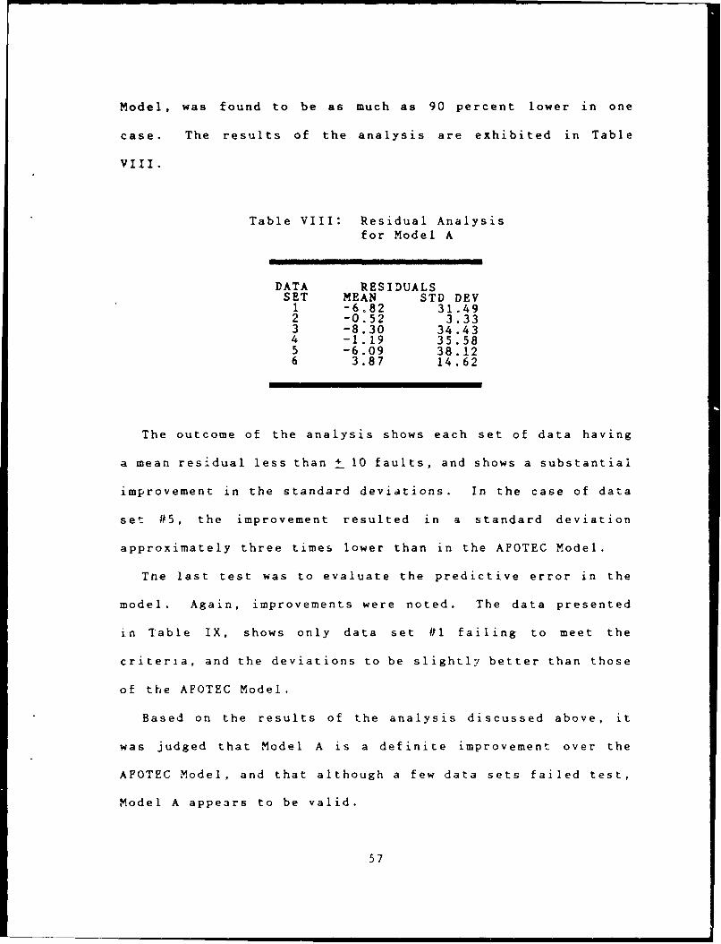
Model, was found to be as much as 90 percent lower in one
case. The results of the analysis are exhibited in Table
VIII.
Table VIII: Residual Analysisfor Model A
DATA RESIDUALSSET MEAN STD DEY1 -6.82 31.492 -0.52 3.333 -8.30 34.434 -1.19 35.585 -6.09 38.126 3.87 14.62
The outcome of the analysis shows each set of data having
a mean residual less than + 10 faults, and shows a substantial
improvement in the standard deviations. In the case of data
set #5, the improvement resulted in a standard deviation
approximately three times lower than in the AFOTEC Model.
Tne last test was to evaluate the predictive error in the
model. Again, improvements were noted. The data presented
in Table IX, shows only data set #1 failing to meet the
criteria, and the deviations to be slightly better than those
of the AFOTEC Model.
Based on the results of the analysis discussed above, it
was judged that Model A is a definite improvement over the
AFOTEC Model, and that although a few data sets failed test,
Model A appears to be valid.
57

Table IX: Analysis of Predictionsfor Model A
DATA RESIDUALSSET MEAN STD DEV1 36.36 4.222 1.24 4.413 -2.23 39.684 5.25 18.915 -6.89 4.326 -5.87 5.67
58

Appendix B: Analysis of Model B
Introduction
This appendix considers a piece-wise model (Model B) that
follows the S-shaped pattern of the data. This model could
be useful in demonstrating when a program has advanced past
the initial stages of testing and into a steady state. The
results found in this appendix verify the validity of the
piece-wise model.
Description
Model B is used by dividing the data into two sets. The
first set of data is regressed against the equation:
Y = exp(c * t) (15)
where
Y = cumulative number of faultsc = a constant representing the fault detection ratet = time in consecutive days
This first part of the model helps predict when testing will
reach full capacity. The testing is assumed to reach full
capacity at the time, to, when the graph begins to climb
rapidly.
After the testing has reached a steady state, the following
equation is used to model the discovery of software faults:
Y : exp(c * t0) + a' l-exp[-b(t-t ])) (16)
where
Y cumulative number of faultsr, a constant representing the fault detection rate
tO the at which the model switches from the start-upphase to the full scale testing phase
59

a' = a - exp(c * tb = the fault detection rate for full scale testingt = time in consecutive days
Before using this second portion of the model, the time to
reach full scale testing (to must be determined from Equation
(15). Now, a nonlinear regression of Equation (16) is
performed to determine the values of a' and b. Finally, an
estimate of the total number of faults can be calculated
using:
a = a' + exp(c * to (17)
and the mean time between fault estimated by Equation (3O).
The independent and dependent variables for this model are
determined similarly to that in Model A.
It should be noted that Equation (16) is the same as the
equation used in Model A, except the model is shifted up by
the amount of faults detected during the start-up phase, and
shifted right by the amount of time elapsed during the start-
up phase. This shifting was not present in Model A, because
the initial portion of data was discarded.
Results
The results of the validity analysis performed on Model B
are approximately the same as the results for Model A.
presented in Appendix A. The similarity in results is due to
the similarities in the two models and the shifting discussed
above. The two models are exactly the same except for this
shifting that occurs in Model B. For example, if a set of
60

data did not have a start-up phase, Equation (16) would
simplify to be equivalent to Equation (9). Model B,
therefore, is also judged to be a valid method of estimating
the reliability of software.
61

Appendix C: APOTEQ Paper
Predicting System Reliability:Software &nd Hardware
1r. J. WiltseCapt N. UchersonCapt 9. Holaquist
Abstract - This paper presents a practical method of combining software maturity
data with hardware failure data to predict system reliability. Currently, the
Air Porce Operational Test and Evaluation Center (APOTIC) considers software
to be 100 percent reliable for system reliability projections and therefore,
these projections are based solely on hardware failure data. le propose coupling
the results of a hardware model with the results from a decreasing software failure
rate model with imperfect debugging. Software maturity data gathered during
developmental and operational testing is used as input to the software failure rate
model. The effects from software enhancement; developed during the block release
cycles and fault introduction through error correction are added to give a comprehensive
yet practical measure of software reliability, These factors give the software model a
predictive capability that some models lack. An estimate of the total number of faults in
a software system is determined from the failure rate and a software mean time between
critical failure (NTBCF) is defined.
A review of classic hardware reliability modeling used during the development
and oi itional test phase is presented first. Hardware reliability is discussed
intluding previous treatment of software failure data. This is followed by a
description of methods used to demonstrate and project software reliability. Finally,
a discussion on combining hardware and software reliability model results to derive a
system reliability number is presented. An example reinforces the ideas presented.
62

Predicting System Reliability:Software and Hardware
by
J. D. ViltseM. McPherson
1. Holmquist
1. INTRODUCTION
System reliability can be defined in terms of mean time between critical
failure (MTBCP). In specifying a system reliabiliy requirement, the user
states his needs for a mature system. Since the system does not mature for
years after operational test, the mature system reliability required by the
user is predicted from the operational test data. More systems are becoming
software intensive; therefore, the software effects on the overall system
reliability must be considered. The reliability of the software in Department
of Defense (DOD) systems is demonstrated during operational testing but seldom
predicted.
During developmental and operational tests the systems are normally not
mature and the reliability requirements stated are for a mature system.
Therefore the reliability demonstrated during test is used to project the
mature reliability. During each test, all failure data is collected. This
data is then analyzed and each failure is categorized as either critical or
non-critical. We then calculate the mean time between critical failure for the
system using all the critical failures observed during the test. The critical
failures can include both software and hardware failures. A demonstrated MTBCF
is reported based on these failures.
To project the reliability to maturity, defined as initial operational
capability (10C) plus two years, the testers use a reliability growth program
63

specified and funded by the system program office. The reliability growth plan
used varies from program to program. Many use the Duane Growth Model, others
use the Army Materiel Systems Analysis Activity (AMS11) Model, or engineering
analyses. Ihichever model is specified, the data is analyzed to determine if
the model fits the data. In projecting to maturity, all software fsults are
considered fixed. So the projected MTBCF includes only hardware failures. In
reporting the projected MTBCF, the testers report the point estimate, as well
as the confidence limits, for the reliability, if possible.
Current test and evaluation methodologies assume all software faults will be
fixed by system maturity. System reliability is therefore projected solely on
the basis of hardware failures. An erroneous picture of system reliability is
presented to the user and senior decision makers as shown in Figure 1. System
reliability is typically presented as a demonstrated system HTBCF which
includes both hardware and s, tware. For predicting future system reliability,
the software is assumed to be perfect (as shown by the step function Delta 1)
and hardware reliability is then grown to a mature value. This leads to a
misconception that the grown hardware reliability is the system reliability.
If software is properly accounted for in total system reliability, the mature
system MTBCF will be lower (Figure 2) by Delt, 2. The effect that software has
on system reliability has been long overlooked and must be addressed since top
level decision makers are now asking if the system reliability projection
includes the software's contribution.
Presently, there are many methods for predicting software reliability, most
of which fit into the following categories: Time between failure models,
failure count models, fault seeding models, and input domain models. In
developing a model to be used at AFOTIC, practical features from existing
64
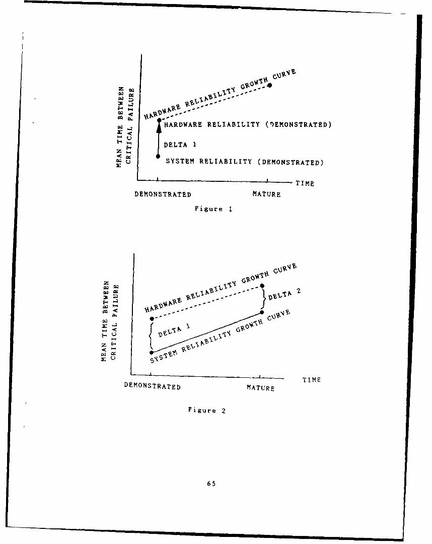
CO HARDWARE RELIABILITY (D)EMONSTRATED)
DELTA 1
Q SYSTEM RELIABILITY (DEMONSTRATED)
TIME
DEMONSTRATED MATURE
Figure 1
z JIlt GIL3*"v
DEMONSTRATED MATURE TM
Figure 2
65
|w |Q Ks| 2. |m ! i i I I

models were combined with our maturity method as well as other
constraints.
A BRIEF DISCRIfTION OF SOFTVARE KATURITY
Software maturity is a measure of the software's progress in its evolution
toward meeting user requirements. Several development indicators give insight
about this progress. The rate at which software errors are being discovered
and fixed is the primary indicator of software maturity.
Software changes are made to correct errors in the software design and
programming. Errors result in deficiencies which we will call faults. Each
fault has a unique impact in the system and is categorized by one of five
different DOD standard severity levels with associated weights (Figure 3).
Severity levels range from minor inconveniences to major problems that can
cause system abort. The faults (or changes) are multiplied by their respective
severity weight to produce values called 'change points". The accumulated
change points are tracked over time. Two curves: Originated and Closed are
plotted which illustrate software maturity (Figure 4).
The Originated curve is determined by accumulating the first occurrence of
each change point plotted versus time. The greatest software change rate occurs
early during software testing. As problems are worked out of the software,
this change rate decreases to some steady-state value. The slope of the curve
decreases with time because the rate of discovering errors, and the severity of
those errors, decreases with time.
In addition to plotting software changes over time, we plot a second curve
(called the "Closed" curve) based on software changes implemented or fixed.
This gives an indication of the rate at which software faults are corrected
compared to the rate at which they are being discovered. The faults that have
66

Severity SeverityLevel Severity Description Weight (Points)
I System Abort. A software of firmware problem that 30results in a system abort.
2 System Degraded. A software of firmware problem that 15No lork-around. severely degrades the system and no
alternative work-around exists (programrestarts not acceptabie).
3 System Degraded. A software of firmware problem that 5Work-around, severely degrades the system and there
exists an alternative work-around(i.e. system rerouting through operatorswitchology; no program restarts).
4 Software Problem. An indicated software of firmware problem 2System not that does not severely degrade the systemDegraded. or any essential system function.
5 Minor Fault. All other minor deficiencies of non-functional faults.
Figure 3
-ORIGINATED
--- CLOSED
z
z
" TIME
Figure 4
67

been corrected are weighted using the same severity scale as the faults that
have been discovered. As the software matures, the gap between the Originated
and Closed curves should narrow (this concept is referred to as 'closure').
The minimum data required for the software maturity metric consists of the
following:
1) Software problem number - a unique identifier used to distingush
one software problem from another.
2) Affected software configuration item - the particular program
where the software problem was discovered.
3) Severity of the problem - a numeric value (1 thru 5) of the impact
the software problem has on the system.
4) Date of initial discovery - the date the software problem was
identified.
5) Date problem was fixed - the date the software problem was closed.
6) Description of problem - short narrative describing the software
problem (needed for traceability between software problems).
To use software maturity data for software reliability, we use only severity
level I and 2 software faults without the weighting factor.
2. MODEL DIVELOPMENT
A model is required to determine the effect of software critical failures
on system reliability assessments. The fact that AFOTEC is an operational test
organization insists that we choose a method that uses actual operational test
data to make a software reliability prediction. Also, we need to choose a
68

method that allows us to relate failure data to calendar time which is a
constraining factor of some models. Also, this methodology must use system
level observables and existing failure reporting systems. Critical failure
data are to be taken from the software maturity data collected during testing.
Historical software maturity data has exhibited an "xponentially decreasing
failure rate process. Reliability assessments for systems containing both
hardware and software must be based upon compatible mathematical foundations and
a consistent set of terms ahich suggests that the chosen must be of an
exponential nature. We emphasize the selection and development of a software
reliability assessment model which is most compatible with hardware reliability
theory and practice.
BASIC MODEL
An exponentially decreasing failure rate process is central to the model me
hve chosen. Based on the above considerations, a description of the software
failure rate prncess as proposed by Goel and Okuuoto was selected as the core
of our model which has the following form:
m(t) : a(l - e bt) (1)
where m(t) is the expected :ccumulated number of critical software faults at
any time t, a is the total number of critical software faults (a constant) in
the system to be observed eventually, and b is the fault detection rate per
fault (also a constant). Musa has demonstrated the validity of using calendar
time in software reliability modeling. We have observed this same failure rate
process across calendar time in APOTEC's software maturity data.
69

This basic model assumes that each fault causes only one failure and is
corrected before causing a second failure. lithout further modification, this
model also assumes that each fault is fixed perfectly (i.e. no new faults are
introduced as a result of fixing a fault) and that there are no faults
introduced whenever it enhancement is made. '.adificat.on to the basic model
which address impertect debugging and errors introduced from enhancements will
be presented.
To use this model in a predictive mode, we curve fit software maturity test
data to equation (1) and obtain the constants a and b. This equation is then
differentiated to obtair the new fault discovery rate to give the following:
dm(t)/dt = abe-bt (z)
Next the time (t) at system maturity is used in the above euation to obtain
the new fault discovery rate at system maturity which is the reciprocal of the
MTBCF for software. This M7BCF can be combined with the hardware M'7BC for an
initial combined system RTBCF (figure 5).
In order to calculate an overall system PITBCF, we first project the
hardware MTBCP to maturity using whichever model has been specified for the
system, and project the software RTBCF using the method descrihed earlier.
The next step is to pic, an arbitrary time period, t, and determine the number
of failures that should occur during the period. To do this use the follo.ing
equations:
Number of hardware failures in time period t = t/MTBCPFW
Number of software failures in time period t = t/MBcr:w
70
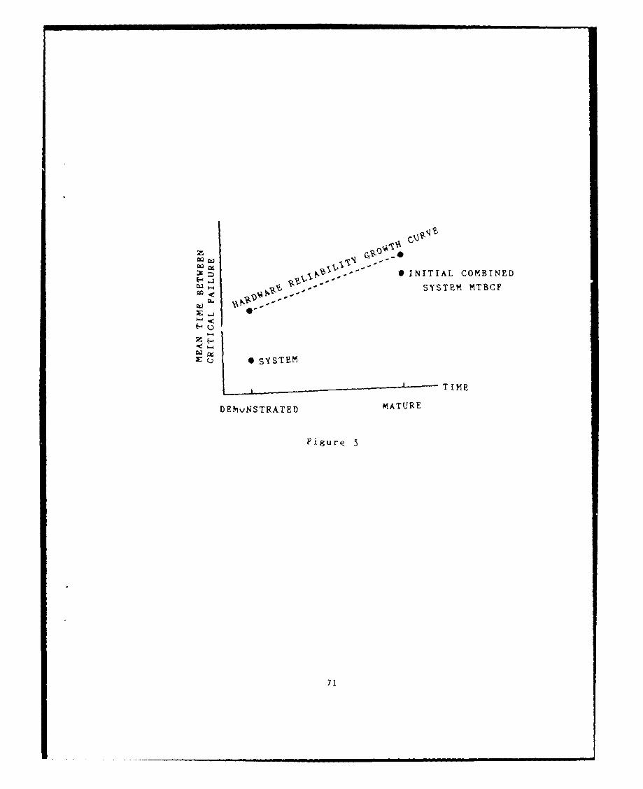
CJ3,,o t
* INITIAL COMBINED
Nq- SYSTEM MTBCF
0 SYSTEM
TIME
DEfvNSTRATED MATURE
Figure 5
71

These are combined to give the total number of failures occurring in time
neriod t.
Total number of faiiures = t/MTBCFHB+ t/MTBCF 3
To get the combined system MTBCF, divide the total number of failures into the
time t.
MTBCPSYS = t It + t 1 + I
MTBCHw MTBCF S1 MTBCF OV MTBCF SI
The MTBCPsYsis the projected system mean time between critical failure.
IMPERFECT DEBUGGING
To increase the predictive accuracy of this model, we need to eliminate as
many constraining assumptions as possible. The assumption that when fixed a
fault is fixed correctly and no new faults are introduced as a result of fixing
a software fault may be removeJ if we introduce a consideration for imperfect
debugging. The latter of these two is more closely akin to the introduction of
new faults when enhancements are made and will be treated in that paragraph.
The consideration for imperfect debugging describes the effect on software
reliability when a fault is not fixed correctly. In an application of Musa's
method for addressing imperfect debugging the average of the fault
correction/fault detection ratio collected over the life of the test gives an
error reduction factor (B). Musa states 'it appears likely that B may not
vary from project to project" and gives 0.96 as a value. Errors not correctly
fixed are treated as additional errors and therefore an increase in the
72

constant a is necessary. This is done by dividing the constant a by B in
equations (1) and (2) to obtain the constant a' which changes these equations
to the following:
'(t) = a'(1 - e-bt) (3)
and
dm'(t)/dt = a'be -bt (4)
where
a' = a/B
This will give a smaller NTBC? for software and thus for the system.
ENHANCEMBNTS
The assumption that no new faults are introduced as a result of changing or
enhancing the software may be removed by adding a factor to account for
software enhancements as suggested by Hecht. The initial fault content of the
enhanced code is proportional to the fault content of the original code. This
means a straight multiplicative factor may be used in determining the final
fault count (the constant a'').
m"(t) a''(1 - e-bt) (6)
and
dm''(t)/dt = a'be-bt (7)
73

The basic model combined with imperfect debugging and enhancements will give a
final software HTBCF. THis final software RTBCY can be combined with the
hardware MTBCF for a final combined system HTBCF (Figure 6a).
3. DISCUSSION$
What makes this approach different from previous software reliability
models and methods is the way it is applied and presented to decision makers.
Instead of giving a single reliability number, a confidence interval for system
reliability (including software) is presented. Since the most conservative
estimate of software reliability is derived from the basic model, the value
produced is combined with the hardware r liability to give the upper limit of
the confidence interval. The lower bound of the confidence interval is derived
by combining the value produced by the complete model (including the imperfect
debugging and enhancement effects) rith the hardware reliability projection.
Figure 6b gives a pictorial representation of system reliability showing the
confidence interval provided by including software reliability. Presenting the
data in this manner allows the decision maker to consider software in the
system reliability projection without being held to a specific number. This
estimate of software's contribution to the system reliability projection will
be conservative (i.e. because of the limiting assumptions, the system will have
more software critical failures than predicted by this model). Although this
method does not perfectly present all aspects of software on system
reliability, it does address the more significant contributions of software on
the system reliability.
74

Z ma INITIAL COMBINED0 SYSTEM MTBCF
NV~-- -0 FINAL COMBINED'
Cc SYSTEM MTBCF
-
*SYSTEM
TIME
DEM'ONSTRATED MATURE
Figure 6a
~CONFIDENCE INTERVAL
TIME
DEMONSTRATED MATURE
Figure 6b
75

4, SUMMARY
Software fault data identified throughout testing is used to assess the
maturity of system software. Software maturity trend data, which is readily
collectable during test, can also be used for software reliability modeling. A
basic decreasing failure rate model coupled with compensation mechanisms for
imperfect debugging and future enhancementg ;s useful for presenting software's
contribution to system reliability. A confidence interval which shows the
range of software's effect on system reliability is an acceptable way of
introducing software into the system reliability projection.
76

Appendix D: List of Acronyms and Symbols
AFIT Air Force Institute of TechnologyAFOTEC Air Force Operational Test and Evaluation
CenterAFR Air Force RegulationAFSC Air Force Systems CommandAJPO Ada Joint Program OfficeASD Aeronautical Systems Divisiona Total expected number of software faultsa' a/B
b Fault detection rate per faultB Musa's constant, 0.96
CPCI Computer Program Configuration ItemCPU Computer Processing Unit
DOD Department of DefenseDTIC Defense Technical Information Center
ENIAC Electronic Numerical Integrator andCalculator
E Average instruction execution rateE0 Initial number of errors in the program
f E/I
HOL Higher order languageh(t) Failure rate
I Total number of machine languageinstructions
INFOCEN Information Center
K Constant of proportionality
MSE Mean square errorMTBF Mean time between failuresMTBFsyS MTBF of the systemMTBFHW MTBF of the hardwareMTBFsw MTBF of the software
77

M(t) Cumulative number of failuresM'(t) Fault discovery rate
N Initial number of errorsn Total number of faults corrected by time, tNASA National Aeronautics and Space
Administration
OT&E Operational Test and Evaluation
PROC NLIN Nonlinear regression procedure
R&M Reliability and MaintainabilityRADC Rome Air Development CenterR~t) ReliabilityR Coefficient of Determination
SAS Statistical Analysis SystemSEI Software Engineering InstituteSSE Sum of square errorsSST Total sum of squareSTARS Software Technology for Adaptable Reliable
Systemsse Standard deviation of residuals
t Cumulative time on test
xi Debugging time between the (i-l)st and itherror
78

Appendix E: Graphs and Data Plots
PLOT OF FAIL*TIME SYMBOL USED IS APLOT OP YHAT*TIME SYMBOL USED IS P
A330 + AA
AAAAAA
300 + AAA
AAAA
AA270 + AA PPP
AA PPA PPPA PPP
240 + A PPA PP
P AAPPR APE 210 + PPPD PPPAAI PPP AAC PP AT 180 + PP AAE PP AD PPP AA
PP AAV 150 + P AA PPP AAAL PP AAU PP AAE 120 + PP AA
P P AAPP AAA
PPP AA A90 + PP A
P AAAPPP A AA
PP AA60 + P AA
P APP AA
P AAA30 + P A
P AAPP APAA A A
0 +P A+- -..... ..... + .... .... .... .. -. - - +.. ..-- +.....--_
0.0 0.2 0.4 0.6 0.8 1.0 1.2 1.4 1.6 1.8 2.0
TIME
Figure 12: Model versus Actual for AFOTEC
Model (Data Set #I)
79

PLOT OF PAIL*TIME SYMBOL USED IS APLOT OF YHAT*TIME SYMBOL USED IS P
45 +
40 +A
AAA?
35 + A
APAP
AP 30 + ARE APD P
C 25 +TB PD
P
V 20 +AL AU PA
E15 +
10 + A
A
PA
P+A
A
0 +-4---------+---------------------------------------------------+-------------------4---
0.0 0.1 0.2 0.3 0.4 0.5
TIME
Figure 13: Model versus Actual for AFOTEC
Model (Data Set #2)
80

PLOT OF IAIL*TIME SYMBOL USED IS APLOT OF YHAT*TIME SYMBOL USED IS P
900 +
800 +
AAAA
AAA
700 + AAAA
AAA PP
A PPP 600 + A PPPR AA PPPE A PFPD A PPI APPC 500 + PPAT PPPAAE PPP AAD PPP A
PPP AAAV 400 + ppp A
A PPP AA
L PPP AU PP A
E PP A300 + PP AA
PP AAPP AA
P AAPP AA
200 + PP AAPP A
P AA
P AA100 + P AAAAAAAA
P AAAPP A AAAAAAA A
APPAAAAPP
0 +PA--- + +## ------------ ------------------------------------------
0.0 0.2 0.4 0.6 0.8 1,0 1.2
TIME
Figure 14: Model versus Actual for AFOTECModel (Data Set #3)
81

PLOT OF FAIL*TIME SYMBOL USED IS APLOT OF YHAT*TIME SYMBOL USED Iq P
1100 +
1000 +
AAAA
900 + AAA
AA PAA PPP
AAPP800 + APP
A APP AR AE 700 + AD A PP
I APPPC PPT 600 ?APE PPPAD PPAA
PP AAV 500 + PPP A
A PPP AL PPP AAU PPP AAE 400 + PP AA
PPP A
PP AAPP AA
35+ PP A
PPP AAPPe AAA
PP AA200 + P A
PP APPP AAA
PP AAA100 + P AAAA
PP A AAAPP AAAAAAPAAAAA
0 +APA--- +- +---+---- ---- ------
C.0 O l 0.2 0 3 0.4 0.5 0.b 0.7
TIME
Figure 15: Model versus Actual for AFOTEC
Model (Data Set 44)
82

PLOT OF VAIL*TIME SYMBOL USED IS APLOT OF YHAT*TIME SYMBOL USED IS P
1300 +
A1200 + AA
AAAA
1100 + AAAAA
AAP 1000 + AA
R AAE A PPD 900 A PPPI AA PpPC A PPPPT 800 APPPE AAPD PPA
700 + PPPAAv PPPP AAA PPP AAL 600 + PPP AA
U PPP AAAE PPP AAA
500 +PPP AAAPPP AA
PPP AAAAA
400 + PPP APP A
PPP AAA300 + PPP AAA
AAAAAAA
200 PP AAPP A
AA100 + P A AA
AAAA
0 PA A A----- -+---- ---- +----
0.0 0° 1.0 1.5 2.0 2.5
TIME
Figure 16: Model versus Actual for AFOVEC
Model (Data Set 05)
83

PLOT OF FAIL*T.-ME SYMBOL USED IS APLOT OF YHAT*TIME SYMBOL USED IS P
180 +
A160 + AA
AAAA
140 + AA PA PAA P
A PPAA 'P
P 120 + AA PPR A PPE AA PD A PPI A PPc 100 + AAP FT APE PAPD PPAA
PAAV 80 + P1, AA
A PAA AL PPAAU PP AE PP AA
60 PPP APP A
P AAAA
40 + A
AAA
A
A20+ P A
AAAAA
A AA0 +AP
---.- - -+-.. .-- .+.-.--- + - ....----------.- --------
0.0 0.2 0.4 0.6 0.8 1 0 1.2 1.4 1.6 1.8
TIME
Figure 17: Model versus Actua; for AFCTECModel (Data Set Ph)
84

PLOT OF PAIL*TIMB SYMBOL USED IS A
PLOT OF YHAT*TIME SYMBOL USED IS P
330 +
300 +
AAAAA
270 + AA
AAAAAAAA P
240 + A PPAA PPP
P A PPR AAPPE 210 + APP
D PAPI PPPAC PP AAT 180 + PP A
E PP AD PP AA
PP AV 150 + PP A
A PP AA
L PP AAU PP AAAAE 120 + P AA
PP AAAPP AA
P AA90 + PPP AA
PP A AAPP AAA
P AAA60 + PP AAAA
P PAAPP A
PPAA30 + PAA
AP AA
PA0 +PA
-- .-----------------------------------------------------------
0.0 0.2 0.4 0.6 0.8 1.0 1.2 1.4
TIME
Figure 18: Model versus Actual for
Model A (Data Set #1)
85

PLOT OP IAILTIME SYMBOL USED IS APLOT OF YHAT*TIME SYMBOL USED IS P
45 +
40 +A
AAAP
35 + A
APAP
AP 30 + ARE APD PIC 25 +TE PD
P
V 20 +AL AU PAE
15 +
P
10 + APA
PA5 + A
A
0 +-4------------------------+-------------------+-------------------------------------
0.0 0.1 0.2 0.3 0.4 0.5
TIME
Figure 19: Model versus Actual for
Model A (Data Set #2)
86

PLOT OF PAIL*TIME SYMBOL USED IS APLOT OF YHAT*TIME SYMBOL USED IS P
700 + Pp
P AAAAAAAP
AAAAAPPP
P 600 + AAA PR AA PPPB AA PPD A PPI AA PPC 500 + AAPPT APPPPAPPD APP
AAPV 400 + PAA PPAAL PPPAU PP AE PPAAAA
300 + PPA
PAAPP A
PPPAAP A
200 + PP AAPP AA
PPPAAPPAAA
PPPAA100 + P AA
PPAAAAAA
PPAAA
0 +P AA----------------------- -------------- ----- +-------------
0.0 0.1 0.2 0.3 0.4 0.5 0.6 0.7
TIME
Figure 20: Model versus Actual for
Model A (Data Set #3)
87

PLOT OF PAIL*TIME SYMBOL USED IS APLOT OF YHA*TIME SYMBOL USED IS P
800 +P
PP
PP AA
700 + PP AAAPPAA
?eAAA
PP AAA
P 600 + AAR A AB AD AAI AC 500 + A
T A PPE AA PPD A PP
AAA PPV 400 + AA PPA A PPL AAPPU AAPE APP
300 + AP
APPA
PAPPAA
200 + PPAAPAA
PPAAPPAAPPAA
100 + PP AAPP AA
PP AAAPPAAAA
PPAAOAA
0 + A b --------------------------- +------------+------------------------
0.00 0.06 0.12 0.18 0.24 0.30 0.36 0.42
TIME
Figure 21: Model versus Actual for
Model A (Data Set #4)
88

PLOT OF FAIL*TIME SYMBOL USED IS APLOT OF YFAT*TIME SYMBOL USED IS P
RED PI APC 500 4 APPAAT A APPAE AAAA PD AAA PP
AAAA PPV 400 + AAA PPPA AA PPPL AAA PPPU A PPPE A APP
300 + AAP PAAPP
AAPPPAP
PPPA
200 + PP AAPP A
PPP AAPPP AA
PP AA100 + PPP AAAA
PPP AAAP A
AAAAAA
0 +P A+------------------------------------ ------- +---------------
0.0 0.1 0.2 0.3 0.4 0.5 0.6 0,?
TIME
Figure 22: Model versus Actual forModel A (Data Set #5)
89

PLOT OF FAiL*TIME SYMBOL USED IS APLOT OF YHAT*TIME SYMBOL USED IS P
P1?(N +
P APP A
110 + P
P
P 100 + P AAR " A AAE PAD 90 + PAI APC PT 80+ A A AE A A PD A
70 + A APV AA PPA A PL 60 + AAPPU AAPPE APP
50 + PA
APAPA
40 + PA
APAP
30 + AAP
AA PAA
20 + AAA PAA P
:A P10 +A P
,A PP,APP
0 +P-------------------------- +------------------------------+----------
0.0 0.2 0.4 0.6 0.8 1.0
TIME
Figure 23: Model versus Actual forModel A (Data Set #6)
90

Appendix F: Research Data Sets
The following are data sets used in conducting the research
discussed in this document. The data found below are in theformat: Date(YYYYMMDD), and the next number is the cumulativenumber of faults detected by that date.
DATA SET #1 (Space System)
19860424 1 19870317 84 19870828 14119860514 3 19870324 85 19870831 14219860530 4 19870327 86 19870902 14419860606 5 19870407 88 19870908 14519860715 6 19870408 90 19870909 14619860905 11 19870409 91 19870914 14719860915 16 19870413 93 19870916 14919860916 17 19870420 94 19870917 15019860922 18 19870429 95 19870920 15119860930 20 19870430 96 19870921 15319861014 24 19870503 98 19870922 15419861016 32 19870505 100 19870924 15519861023 35 19870527 101 19870925 158198LI103 38 19870604 102 19870926 15911361117 39 19870612 103 19870930 16119861119 42 19870615 104 19871001 16319861120 43 19870616 105 19871002 16419861126 44 19870617 106 19871005 16519861201 45 19870618 107 19871006 16719861204 47 19870619 108 19871007 168
19861209 50 19870622 110 19871008 16919861210 51 19870624 111 19871010 17019861215 56 19870625 114 19871012 17119861218 58 19870629 116 19871013 17219861231 59 19870702 117 19871014 17419870102 60 19870706 119 19871015 17519870105 64 19870707 122 19871016 17719870107 65 19870713 123 19871017 17919870108 66 19870715 126 19871020 18319870112 70 19870718 127 19871021 18519870114 71 19870722 128 19871022 18719870121 72 19870728 130 19871023 190
19870203 74 19870730 131 19871025 19119870206 75 19870801 132 19871026 19219870211 76 19870804 133 19871028 19519870217 77 19870805 134 19871029 19619870224 78 19870806 136 19871030 19719870303 79 19870807 138 19871102 19919870309 80 19870810 139 19871104 20019870312 82 19870821 140 19871105 201
91

19871107 202 19880309 30219871109 203 19880315 30319871110 204 19880317 30819871111 205 19880320 309
19871112 214 19880322 31219871113 215 19880323 313
19871114 217 19880325 314
19871115 218 19880329 315
19871116 219 19880331 316
19871117 221 19880404 317
19871118 223 19880406 31819871120 224 19880408 32019871122 225 19880409 32119871125 229 19880413 32219871128 230 19880418 32419871130 232 19880419 32519871207 237 19880421 32619871208 240 19880425 327
19871209 245 19880426 32919871211 248 19880428 33019871212 249 19880503 331
19871214 255 19880504 332
19871215 260 19880506 33319871216 263 19880511 335
19871217 264 19880513 33619871221 26519871222 26719871224 26819880104 27019880108 27219880109 27319880114 27419880115 27519880117 27619880125 27719880126 27919880129 28219880202 28319880203 28419880204 28519880205 28619880208 28719880210 28819880211 29019880215 29119880217 29519880222 29619880227 29719880229 298
19880301 29919880307 30019880308 301
92

DATA SET #2 (Aircraft System)
19870827 219870828 419870829 519870831 619870902 819870905 1019870908 1719870910 1819870914 2819870916 3019870919 3119870921 3319870922 3419870924 3719870925 3819880328 40
93

DATA SET #3 (Communications System)
19870129 3 19870901 104 19871204 34319870130 5 19870910 105 19871207 35019870202 9 19870911 106 19871208 35419870203 16 19870916 108 19871209 36019870204 21 19870918 115 19871210 36219870205 22 19870923 118 19871211 37619870206 23 19870924 121 19871214 38019870209 25 19870925 124 19871215 38519870210 28 19870928 127 19871216 394
19870216 30 19870929 152 19871217 39919870217 32 19870930 156 198712i8 40419870218 33 19871001 159 19871221 41219870219 38 19871005 165 19871222 41519870225 39 19871006 168 19871223 41919870226 40 19871007 170 19871228 42019870302 41 19871008 173 19871229 42219870305 42 19871009 175 19871230 42619870306 45 19871012 177 19880104 42919870313 46 19871013 187 19880105 43619870319 47 19871014 190 19880106 44219870323 48 19871015 196 19880107 44819870331 49 19871016 203 19880109 45919870420 50 19871019 205 19880110 464
19870514 51 19871020 211 19880111 47119870527 52 19871021 217 19880112 47319870603 58 19871023 226 19880113 47619870610 62 19871026 233 19880114 48119870615 63 19871027 236 19880115 48619870619 64 19871029 243 19880118 48919870624 65 19871102 249 19880119 49619870629 66 19871103 253 19880120 50419870702 67 19871104 260 19880121 51519870713 68 19871105 263 19RP0122 52119870714 72 19871106 266 19880124 52419870716 74 19871109 268 19880125 52719870720 77 19871110 272 19880126 53319870722 82 19871111 277 19880127 54119870723 83 19871112 284 19880128 54319870724 85 19871113 287 19880129 54719870728 89 19dil Il 288 19880201 55419870729 91 19871118 296 19880202 55719870730 92 19871119 297 19880203 56519870805 95 19871120 308 19880204 56819870810 96 19871123 315 19880205 574
19870812 97 19871124 320 19880208 58119870813 98 19871125 325 19880209 58419870817 101 19871130 333 19880210 598
19870824 102 19871202 338 19880211 60319870827 103 19871203 339 19880212 605
94
--- -- --

19880215 609 19880608 77019880216 6111988021A 621198802io 62319P3' 21 62513.d0222 62819880223 63119880224 63319880225 64519880226 64819880229 65119880301 65419880302 65819880303 66419880304 67019880307 67419880308 67619880309 68219880310 68819880311 69219880314 69619880315 70019880316 70119880317 70419880318 71019880322 713
19830323 71519880325 72119880329 72219880330 72419880404 72619880405 72719880407 73019880411 73219880413 73519880414 73619880415 74119880418 74319880422 74619880425 74719880502 75319880512 75419880513 75619880516 75719880517 76019880519 76119880520 76319880524 76419880525 76519880527 76619880606 76719880607 769
95

DATA SET #4 (Communications System)
19880328 4 19880627 121 19880829 36710 ,80330 9 19880628 125 19880830 384
19880406 11 19880629 130 19880831 386
19880411 13 19880701 133 19880901 39019880413 16 19880705 136 19880902 39119880414 19 19880706 138 19880904 39219880415 21 19880708 144 19880905 394
IQ 8 80418 22 19880709 145 19880906 40219880419 24 19880711 148 19880907 410
19880420 25 19880712 149 19880908 414
19880421 28 19880713 156 19880909 42119880422 30 19880714 160 19880910 423
19880426 31 19880715 162 19880911 428
19880427 36 19880719 173 19880912 43819880429 39 19880720 177 19880913 441
19880501 40 19880721 187 198809)4 450
19¢80503 41 19880722 192 198809i5 461
19880504 42 19880723 196 19880916 474
19880505 45 19880724 197 19880917 483
19880506 47 19330725 204 19880919 494
19880509 50 19880726 213 19880920 498
19880510 56 19880727 217 19880921 50619880512 57 19880728 224 19880922 52119880516 58 19880729 227 19880923 52619880517 59 19880801 228 19880926 531
19880518 60 19880802 233 19880927 53919880519 62 19880803 237 19880928 549
19880524 63 19880804 239 19880929 55419880526 66 19880805 241 19881002 5551;880527 69 19880808 245 19881003 565
19880602 73 19880809 249 19881004 58319880603 74 19880810 255 19881005 590
19880606 76 19880811 257 19881006 60019880607 77 19880812 264 1988100' 61519880608 81 19880813 266 19881008 61619880609 83 19880815 269 19881010 62119880610 85 19880816 273 19881011 62619880613 86 19880817 284 19881012 64319880614 91 19880818 294 19881013 64719880615 92 19880819 297 19881014 659
19880616 93 19880820 307 19881015 661
19880617 94 19880821 309 19881017 66319880618 96 19880822 318 19881018 66819880620 99 19880823 322 19881019 674
19880621 104 19880824 328 19881020 68019880622 108 19880825 335 19881021 688
19880623 110 19880826 343 19881024 69219880624 112 19880827 354 19881023 69319880625 115 19880828 361 19881024 704
96

19881025 710 15890129 10891)881026 722 19890130 109319881027 734 19890131 110019881028 74019881029 74219881031 76519881101 76719881102 77519881205 77619881206 78919881207 7941vi81208 79919881209 81519881212 82419881213 84119881214 84619881215 85719881216 86019881217 86219881218 863198812:; 87719881220 88219881221 88919881222 89419881227 89e19881228 90419881230 90519890103 90919890104 92019890105 93119890106 93819890107 94719890108 94819890109 95919890110 96819890111 98619890112 99119890113 100019890114 100219890116 102019890117 102719890118 103619890119 104619890120 105319890121 105419890122 105519890123 105819890124 106619890125 107419890126 107919890127 108519890128 1086
97
• - mm~m~mmmmm m m m m m m ( mI
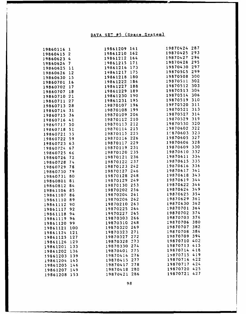
DATA SET #5 (Space System)
19860116 1 19861209 161 19870424 287
19860415 2 19861210 162 19870425 293
19860623 4 19861212 164 19870427 294
19860624 7 19861215 171 19870428 295
19860625 11 19861216 173 19870430 297
19860626 12 19861217 175 19870505 299
19860630 15 19861218 180 19870508 300
19860701 16 19861222 186 19870511 302
19860702 17 19861227 188 19870512 303
19860707 18 19861229 189 19870513 304
19860710 21 19861230 190 19870514 306
19860711 27 19861231 195 19870519 310
19860713 28 19870107 196 19F70520 311
19860714 31 19870108 199 19870521 313
19860715 36 19870109 206 19870527 314
19860716 41 19870112 210 19870529 319
19860717 50 19870113 212 19870530 320
19860718 51 19870114 215 19870602 322
19860721 55 19870115 225 10870603 323
19860722 59 19870116 226 19870605 327
19860723 63 19870117 229 19870606 328
19860724 67 19870119 231 19870609 330
19860725 66 19870120 235 19870610 332
19860726 72 19870121 236 19870611 334
19860728 74 19870122 237 19870615 335
19860729 78 19870123 242 19870616 336
19860730 79 19870127 246 19870617 341
19860731 80 19870128 248 19870618 343
19860801 81 19870129 249 19870619 344
19860812 84 19870130 253 19870622 346
19861106 85 19870202 256 19870624 349
19861107 86 19870204 261 19870625 354
19861110 89 19870206 262 19870629 361
19861112 90 19870210 263 19870630 362
19861117 92 19870225 264 19870701 364
19861118 94 19870227 265 19870702 374
19861119 96 19870303 266 19870703 376
19861120 99 19870310 268 19870706 380
19861121 100 19870320 269 19870707 382
19861124 121 19870323 271 19870708 384
19861125 127 19870327 272 19870709 394
19861126 129 19870328 273 19870710 402
19861201 133 19870330 274 19870713 415
19861202 136 19870401 275 19870714 418
19861203 139 19870414 276 19870715 419
19861204 145 19870415 277 19870716 422
19861205 146 19870417 278 19870717 424
19861207 149 19870418 280 19870720 425
19861208 153 19870421 286 19870721 427
98

19870722 428 19880106 552 19880325 69619870724 429 19880107 553 19880328 69819870727 430 19880108 554 19880329 70019870812 432 19880109 555 19880330 70119870813 433 19880110 556 19880331 70219870815 434 19880112 558 19880402 70319870825 435 19880113 560 19880404 70519870904 436 19880114 561 19880405 71019870910 438 19880115 564 19880407 71619870917 441 19880116 567 19880408 72219870918 446 19880117 568 19880410 72319870921 447 19880119 570 19880411 73119870922 455 19880122 575 19880412 73319870923 456 19880125 577 19880413 74019870923 460 19880126 578 19880414 74419870928 462 19880127 579 19880415 74719870929 466 19880128 581 19880418 75219870930 470 19880129 582 19880419 75519871001 471 19880130 585 19880420 75719871005 473 19880201 588 19880422 75919871006 476 19880202 589 19880423 76419871007 479 19880203 591 19880424 76519871009 481 19880204 592 19880425 77219871016 482 19880205 593 19880426 78219871019 486 19880208 596 19880427 79619871026 488 19880211 598 19880428 79919871027 489 19880212 600 19880429 80119871028 490 19880216 602 19880430 80219871029 494 19880217 607 19880502 80819871031 495 19880218 610 19880503 81619871103 497 19880219 613 19880504 82119871109 503 19880222 614 19880505 82719871111 511 19880223 620 19880506 82919871113 516 19880224 625 19880507 83119871117 520 19880225 628 19880508 83319871122 521 19880226 629 19880509 83719871125 523 19880301 631 19880510 85019871130 527 19880302 633 19880511 86019871201 531 19880303 636 19880512 863
19871207 532 19880308 643 19880513 86419871208 533 19880309 646 19880514 86519871210 534 19880311 649 19880516 87119871215 535 19880312 650 19880517 87519871216 537 19880314 672 19880518 87919871217 541 19880315 674 19880520 88619871219 542 19880316 676 19880521 88819871221 543 19880317 677 19880523 88919871222 544 19880318 678 19880524 89619871230 545 19880321 683 19880525 90319871231 546 19880322 687 19880526 90819880104 550 19880323 689 19880527 90919880105 551 19880324 692 19880530 913
99

19880531 918 19880825 1071 19881118 1221
19880601 923 19880831 1075
19880602 925 19880901 107619880607 926 19880902 107819880608 933 19880905 108619880609 937 19880906 108819880610 943 19880907 109019880611 948 19880908 109119880613 951 19880912 109219880614 953 19880913 109319880615 956 19880914 109419880616 958 19880915 109519880617 962 19880916 109819880618 964 19880918 109919880620 966 19880919 110019880621 968 19880921 110119880622 971 19880922 110319880623 976 19880924 110419880624 984 19880927 1109
19880627 986 19880928 1111
19880628 990 19880929 1119
19880629 991 19880930 112319880630 996 19881003 112619880701 998 19881005 1127
19880705 1000 19881006 112819880706 1003 19881007 1130
19880707 1005 19881011 1.14119880708 1013 19881013 1145
19880710 1014 19881014 114619880711 1016 19881017 114719880712 1020 19881018 1151
19880713 1022 19881020 115419880715 1024 19881021 116219880717 1025 19881022 1163
19880718 1029 19881023 116419880719 1030 19881024 116819880720 1033 19881025 116919880721 1034 19881026 117319880722 1035 19881027 117919880724 1039 19881028 118219880725 1042 19881029 1185
19880726 1044 19881101 118619880727 1049 19881102 1187
19880802 1050 19881103 119019880804 1053 19881104 1193
19880805 1057 19881107 119619880809 1058 19881108 1199
19880810 1061 19881110 120019880815 1063 19881114 120419880816 1064 19881115 121019880817 1066 19881116 121319880818 1070 19881117 1218
100

DATA SET #6 (Space System)
19870112 1 19880114 73 19880724 13119870409 2 19880115 74 19880726 13519870902 4 19880117 75 19880729 13719870920 5 19880125 76 19880805 13819870922 6 19880215 77 19880817 139
19870924 7 19880217 79 19880823 14019870925 9 19880222 80 19880826 143
19870926 10 19880227 81 19880831 14419870930 11 19880229 82 19880902 145
19871001 13 19880301 83 19880911 14619871007 14 19880307 84 19880928 147
19871008 15 19880309 85 19881009 14819871012 16 19880315 86 1988122 159
19871013 17 19880320 87 19881026 16019871015 18 19880322 90 19881029 16119871016 19 19880323 91 19881120 16319871017 21 19880325 92 19881123 16419871020 24 19880331 93 19881130 165
19871022 26 19880404 94 19881215 16619871023 29 19880406 9519871025 30 19880408 9719871028 33 19880411 9819871030 34 19880418 9919871102 36 19880418 10019871107 37 19880419 10119871109 38 19880421 10219871110 39 19880425 10619871111 40 19880426 10719871112 41 19880427 10819871113 42 19880428 109
19871114 44 19880504 11019871115 45 19880506 11219871117 46 19880508 11319871120 47 19880510 11419871122 48 19880511 11619871125 49 19880516 11719871128 50 19880521 11819871207 54 19880523 11919871208 56 19880602 12019871209 60 19880605 12119871211 63 19880609 12319871214 65 19880611 12419871216 67 19880614 12519871217 68 19880625 12619871222 69 19880628 12719871224 70 19880629 12819880104 71 19880630 12919880109 72 19880711 130
101

Bibliography
1. Abdel-Ghaly, Adballa A. and others. "Evaluation ofCompeting Software Reliability Predictions," IEEETransactions on Software Engineering. 12: 950-967(September 1986).
2. Air Force Systems Command. Software QualityIndicators. AFSCP 800-14. Andrews AFB MD: HQ APSC,20 January 1987.
3. Air Force Systems Command. Software ManagementIndicators. AFSCP 800-43. Andrews AFB MD: HQ AFSC,31 January 1986.
4. Andrews, Richard A. Class handout distributed inLOG 225, Acquisition Logistics. School of Systemsand Logistics, Air Force Institute of Technology (AU),Wright-Patterson AFB OH, January 1986.
5. Boehm, Barry W. Software EngineerinK Economics.Englewood Cliffs NJ: Prentice-Hall, Inc, 1981.
6. Boeing Aerospace Corporation. "Critical ItemDevelopment Specification for Avionics ComputerController." No. S400-l00-21B. Boeing AerospaceCorporation, Seattle WA, 11 March 1983.
7. Boorman, Scott A. and Paul R. Levitt. "SoftwareWarfare and Algorithm Sabotage," Signal: TheInternational Journal of C31, 42: 75-78 (May 1988).
8. Brocka, Bruce. "An Alternative Paradigm for SoftwareReliability," Reliability Review, 7: 28-29 (June 1987).
9. Department of the Air Force. Acquisition Management:Air Force Reliability and Maintainability Policy.AFR 800-18. Washington: HQ USAF, 1 October 1986.
10. Department of the Air Force. USAF R&M 2000 ProcessAFP 800-7. Washington: HQ USAF, I October 1988.
11. Department of Defense. Military Standard: ReliabilityModeling and Prediction. MIL-STD 756B. Washington:Government Printing Office, 18 November 1981.
12. Department of Defense. Military Standard: DefenseSystems Software Development. DOD-STD-2167A.Washington: Government Printing Office,29 February 1988.
102

13. Department of Defense. Military Standard: DefenseSystems Software Quality Program. DOD-STD-2168.Washington: Government Printing Office, 29 April 1988.
14. Dhillon, B. S. and Chanan Singh. EngineeringReliability. New York: John Wiley & Sons, Inc., 1981.
15. Dunham, Janet R. "Experiments in Software Reliability:Life Critical Applications," IEEE Transactions onSoftware Reliability, SE-12: 110-123 (January 1986).
16. Ferens, Daniel V. "Computer Software ReliabilityPrediction," Proceedings of the IEEE National Aerospaceand Electronics Conference (NAECON): 713-717 (1986).
17. . "Computer Software Fault Tolerance,"Proceedings of the IEEE National Aerospace andElectronics Conference (NAECON): 845-349 (1987).
18. Glass, Robert L. and Ronald A. Noiseux. SoftwareMaintenance Guidebook. Englewood Cliffs NJ: Prentice-Hall, Inc., 1981.
19. Goel, Amrit L. "Software Reliability Models:Assumptions, Limitations, and Applicability," IEEETransactions on Software Engineering, SE-lI: 1411-1423(December 1985).
20. Goldstine, Herman H. The Computer: From Pascal tovon Neumann. Princeton: Princeton University Press,1972.
21. Halpin, John C. "R&M 2000 Changes Customer Prioritiesin Avionics Design," EW Design Engineer's Handbook:Supplement to the Journal of Electronic Defence:5.1-5.3 (December 1987).
22. Hubbard, Col Clarke D., Director of Logistics. PersonalCorrespondence. HQ AFOTEC/LG, Kirtland AFB NM, 15 March1989.
23. Kvalseth, Tarald 0. "Cautionary Note About RThe American Statistician, 39: 279-285 (November 1985).
24. Lewis, E. E. Introduction to Reliability Engineering.New York: John Wiley & Sons, Inc., 1987.
25. Lipow, Myron and Erwin Book. "Implications of R&M 2000on Software," IEEE Transactions on Reliability. R-36:355-361 (August 1987).
103

26. McCarthy, Joseph. "A Software Approach," ProgramManager, 13: 41-44 (May-June 1984).
27. McPherson, Michael R. and others. "Predicting SystemReliability: Software and Hardware," Unpublishedpaper. HQ AFOTEC/LG5, Kirtland AFB NM, November 1988.
28. McPherson, Michael R., Captain USAF. Telephoneinterview. HQ APOTEC/LG5, Kirtland AFB NM,25 May 1989.
29. Mendenhall, William and Terry Sincich. Statistics forkhe Engineer and Computer Sciences. San Francisco:
Dellen Publishing Company, 1984.
30. Moreau, R. The Computer Comes of Age: The People.the Hardware, and the Software. London: MIT Press,1984.
31. Mullins, General James P. "Reliability: Key to CostReduction," Program Manager, 13: 12-16, (September-October 1984).
32. Musa, John D. and others. Software Reliability:Measurement, Prediction. Application. New York:McGraw-Hill Book Company, 1987.
33. Ott, Lyman. An Introduction to Statistical Methods andData Analysis (Third Edition). Boston: PWS-KentPublishing Company, 1988.
34. SAS Institute Inc. SAS User's Guide: Statistics(Fifth Edition). Cary NC: SAS Institute Inc.,1985.
35. Shooman, Martin L. Software Engineering: Design,Reliability, and Management. New York: McGraw-HillBook Company, 1983.
36. Yamada, Shigeru and Shunji Osaki. "SoftwareReliability Growth Modeling: Models and Application,IEEE Transactions on Software Engineering, 7: 1431-1437 (December 1985).
104

I
Captain Charles J. Westgate, III
entered Virginia
Polytechnic Institute and State University. He graduated in
1984 with the degree of Bachelor of Science in Aerospace and
Ocean Engineering, and was commissioned as a Second Lieutenant
in the United States Air Force. After graduation, he was
assigned to the Air Force Acquisition Logistics Center (AFALC)
as an Integrated Logistics Support Manager, until entering the
School of Systems and Logistics, Air Force Institute of
Technology (AFIT), in May 1988. While attending AFIT, Capt
Westgate has also completed a Master of Science Degree in
Management Science at the University of Dayton in August 1988,
and became a Certified Professional Logistician (CPL) in May
1989.
105

UNCLASS IFILED
SECURITY CLASSIFICATION OF THIS PAGE
REPORT DOCUMENTATION PAGE OM o. 070pr 0188
Is. REPORT SECURITY CLASSIFICATION 1b RESTRICTIVE MARKINGSUNCLASSIFIED
2a. SECURITY CLASSIFICATION ALTHORITY1 3, DISTRIBUTION /AVAILABILITY OF REPORT
2b. ECLSSIICATON DOWGRADNG CHEULEApproved for public release; distributionZb. ECLASL~IATIO / DWNGRDINGSCHEULEunl im ited
&. PERFORMING ORGANIZATION REPORT NUMBER(S) 5. MONITORING ORGANIZATION REPORT NUMBER(S)
AFIT/GLM/LSY/89S-7 1
6a. NAME OF PERFORMING ORGANIZATION 6b. OFFICE SYMBOL 7a. NAME OF MONITORING ORGANIZATION
School of Systems and (if applicable)
Logistics I AFIT/LSM_______________________
6c. ADDRESS (City, State, and ZIP Code) 7b. ADDRESS (City, State. and ZIP Code)
Air Force Institute of Technology (AU)Wright-Patterson AFB, Ohio 45433-6583
8.. NAME OF FUNOING/SPONSOR)NG J8b. OFFICE SYMBOL 9 PROCUREMENT INSTRUMENT IDENTIFICATION NUMBERORGANIZATION j(if applicable)
Bc. ADDRESS (City, State, and ZIP Code) 10 SOURCE OF FUNDING NUMBERS
PROGRAM IPROJELT TASK IWORK UNITELEMENT NO. INO. NO IACCESSION NO
11. TITLE (include Security Classification)
VALIDATION OF AN EXPONENTIALLY DECREASING FAILURE RATE SOFTWARE RELIABILITY MODEL
12. PERSONAL AUTHOR(S)Charles J. Westgate, III, M.S., Capt, USAF
13a. TYPE OF REPORT 13b TIME COVERED 14. DATE OF REPORT 'Year, Month, Day) jiS.PAGE COUNTMS Thesis IFROM _____TO - 1989 September 118
16. SUPPLEMENTARY NOTATION
17. COSATI CODES 18 SUBJECT TERMS (Continue on~ reverse if necessary and identify by bNock number)FIELD GROUP SUB-GROUP Computer Program Reliability; Reliability;12__________0_______ Computer Programs; Mathematical Models
19. ABSTRACT (Continue on reverse if necessary and identify by block number)
Thesis Advisor: Daniel V. FerensAssociate ProfessorDepartment of Systems Management
Appr,ed for ~lic r.ease: IAW AFR 190-1.
LNR . EMMEHANZLt C 1 USAF 11 Oct 89Director of Research and ConsultationAir Force Institute of Technology (AU)Wright-Patterson AFB OH 45433-6583
20. DISTRIBUTION /AVAILABILITY OF ABSTRACT 21 ABSTRACT SECURITY CLASSIFICATIONQ3UNCLASSI FIE D/'UNLI MITE D 0 SAME AS RPT. C3 DTIC USERS UNCLASSIFIED
22a. NAME OF RESPONSIBLE INDIVIDUAL 22b TELEPHONE (Include Area Code) 22c OFFICE SYMBOLDaniel V. Fereps, Associate Professor (513) 255-3355 1LSM
DD Form 1473, JUN 86 Previous editions are obsolete. SECURITY CLASSIFICATION OF THIS PAGEUNCLASSIFIED

UNCLASSIFIED
The purpose of this thesis was to determine the validityof a software reliability estimation model proposed by theAir Force Operational Test and Evaluation Center (AFOTEC).During the last forty years of the ccmputer era, the demandfor software has been growing at a rate of twelve percent peryear and about fifty percent of the total life cycle cost ofa software system is attributed to software maintenance. Ithas also been shown that the cost of fixing a software faultincreases dramatically as the life cycle progresses. It wasstatistics like those discussed above that prompted thisresearch.
The research had these specific objectives: the first wasascertaining the soundness of the model's intrinsic logic.The second objective was to run the model with actual failuredata to measure the validity and correlation of the data withthe model. The final objective was to determine theassumptions required to operate the model.
The study found the AFOTEC Model to be invalid; however,improvements and assumptions could be easily applied to makethe model a valid tool for estimating software reliability.Two improvements were proposed for the AFOTEC Model. First,the model should operate with the assumption that the dataused in the model should be data obtained after softwaretesting has reached a steady state. The second recommendationwas to modify the AFOTEC Model to emulate both the start-upphase and the steady state phase of testing.
UNCLASSIFIED