Embed Size (px)
Citation preview
1
Correlations Without Synchrony
Presented by: Oded Ashkenazi
Carlos D. Brody
2
Overview
• Neurological Background
• Introduction
• Notations
• Latency, Excitability Covariograms
• 3 Rules of Thumb
• Conclusion
3
Neurological Background
The Human Brain:
A Complex Organism
4
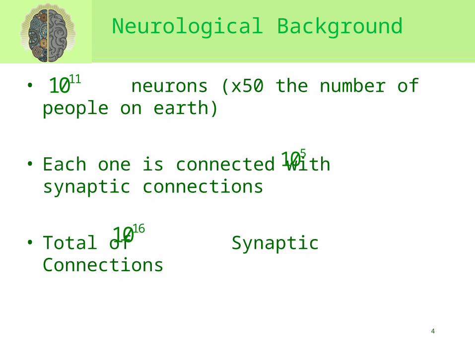
Neurological Background
• neurons (x50 the number of people on earth)
• Each one is connected with synaptic connections
• Total of Synaptic Connections
1110
510
1610
5
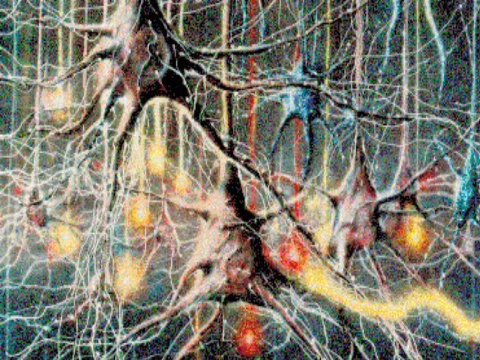
Neurological Background
6
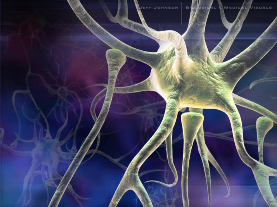
7
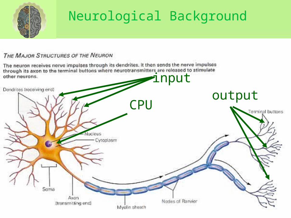
Neurological Background
CPU
inputoutput
8
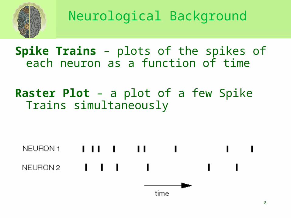
Neurological Background
Spike Trains – plots of the spikes of each neuron as a function of time
Raster Plot – a plot of a few Spike Trains simultaneously
9
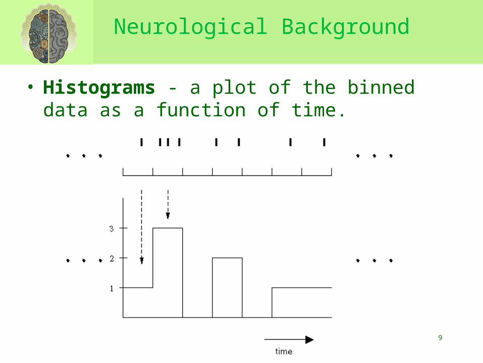
Neurological Background
• Histograms - a plot of the binned data as a function of time.
10
Neurological Background
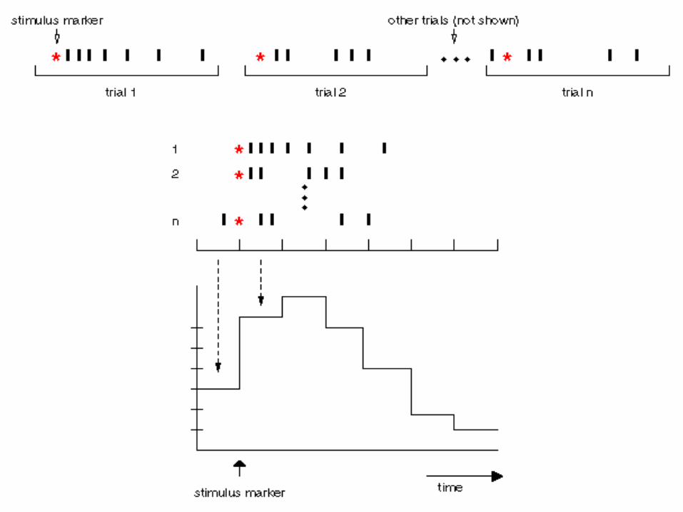
• PSTH - peri-stimulus time histogram
is a Histogram of stimulated neurons lined up by the stimulus marker. (marks the beginning of the stimulus).
• The PSTHs give some measure of the firing rate or firing probability of a neuron as a function of time.
11
12
Neurological Background
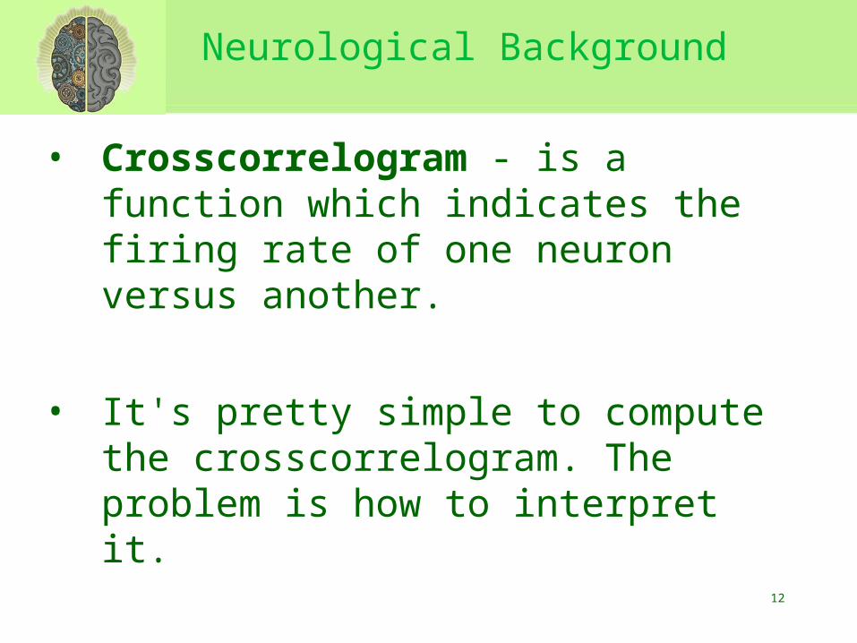
• Crosscorrelogram - is a function which indicates the firing rate of one neuron versus another.
• It's pretty simple to compute the crosscorrelogram. The problem is how to interpret it.
13
Neurological Background
14
Neurological Background
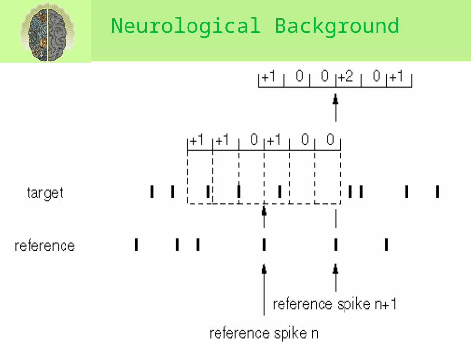
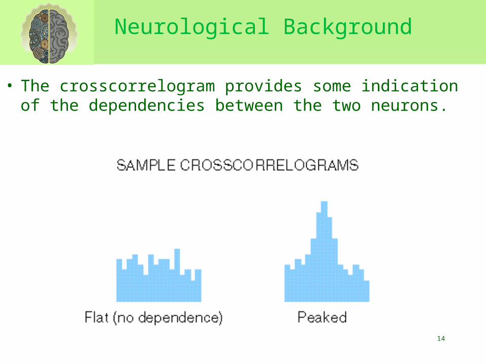
• The crosscorrelogram provides some indication of the dependencies between the two neurons.
15
Introduction
• Peaks in spike train correlograms are usually taken as indicative of spike timing synchronization between neurons.
• However, a peak merely indicates that the two spike trains were not independent .
• Latency or excitability interactions between neurons can create similar peaks.
16
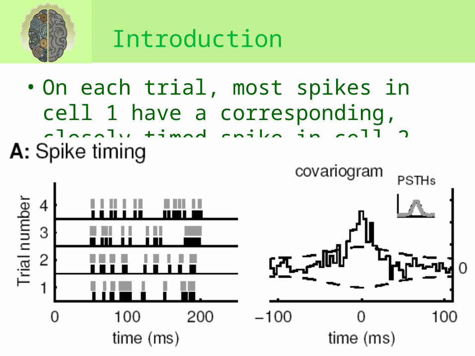
• On each trial, most spikes in cell 1 have a corresponding, closely timed spike in cell 2.
Introduction
17
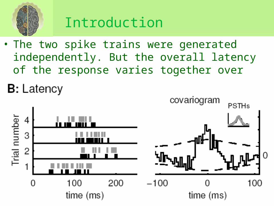
• The two spike trains were generated independently. But the overall latency of the response varies together over trials.
Introduction
18
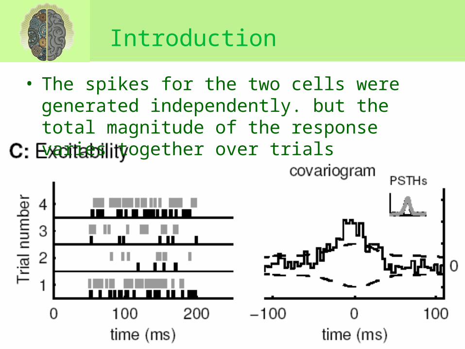
Introduction
• The spikes for the two cells were generated independently. but the total magnitude of the response varies together over trials
19
Notations
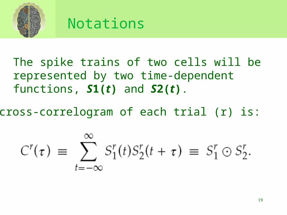
The spike trains of two cells will be represented by two time-dependent functions, S1(t) and S2(t).
The cross-correlogram of each trial (r) is:
20
Notations
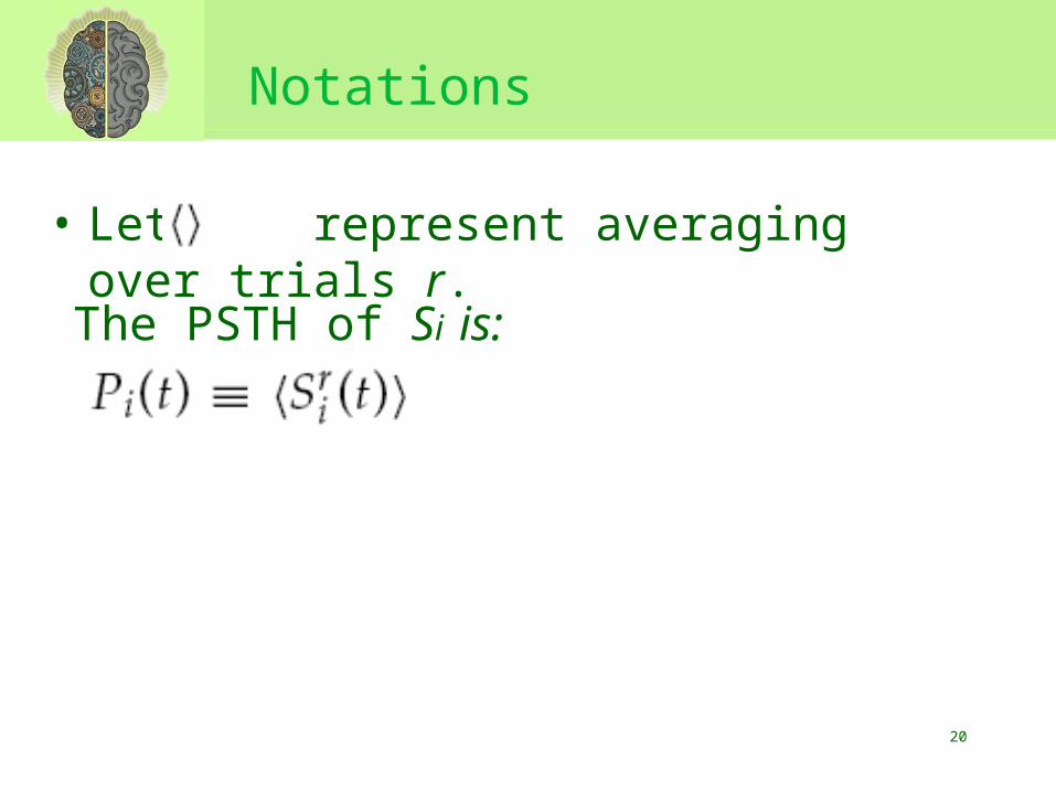
• Let represent averaging over trials r.
The PSTH of Si is:
21
Notations
• When you stimulate the cells that you're recording from, you increase their firing rates.
• If you do this simultaneously in both cells you've introduced a relationship between the firing probabilities of the cells.
• The Covariogram removes the peak in the original correlogram that was due to co-stimulation of the cells.
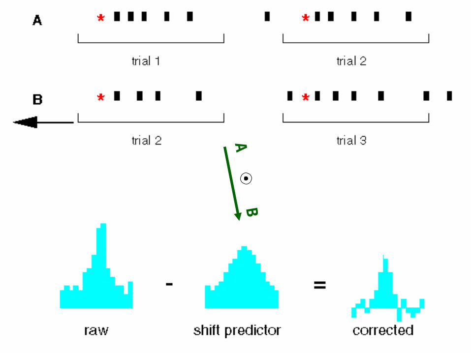
22
Notations
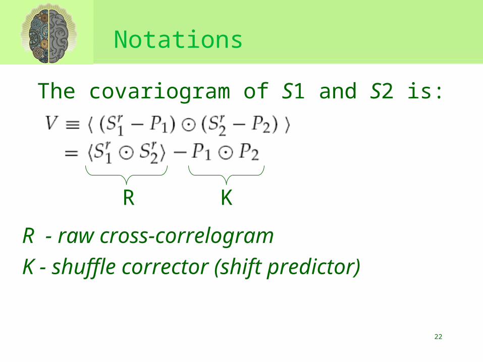
R - raw cross-correlogram
K - shuffle corrector (shift predictor)
The covariogram of S1 and S2 is:
R K
23
A B
24
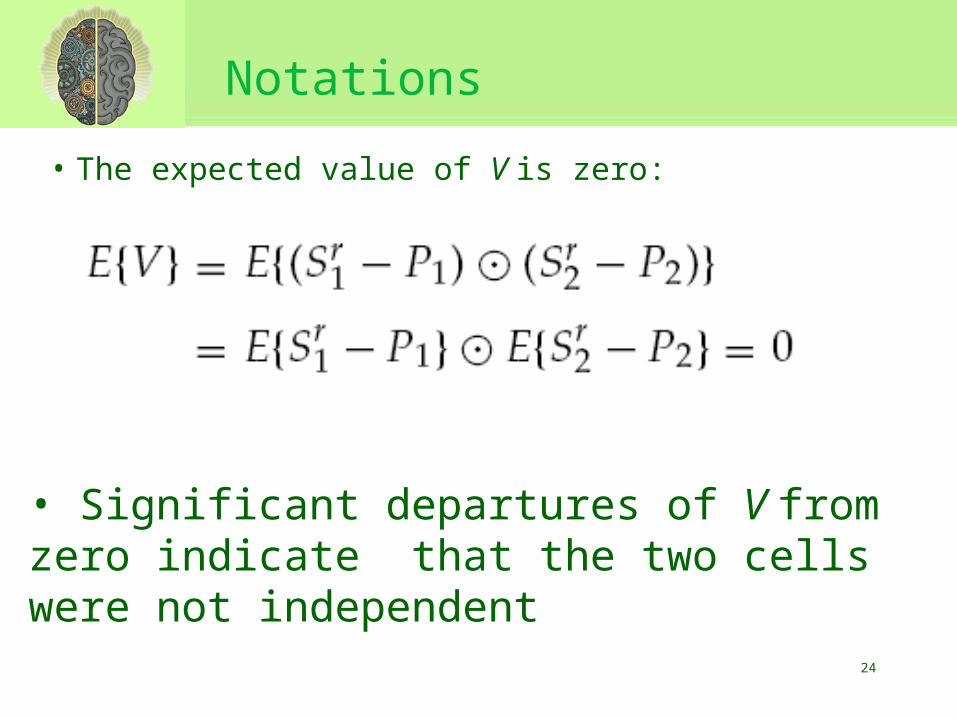
Notations
• The expected value of V is zero:
• Significant departures of V from zero indicate that the two cells were not independent
25
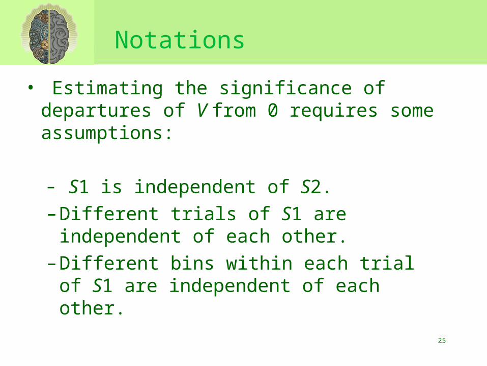
Notations
• Estimating the significance of departures of V from 0 requires some assumptions:
– S1 is independent of S2.
– Different trials of S1 are independent of each other.
– Different bins within each trial of S1 are independent of each other.
26
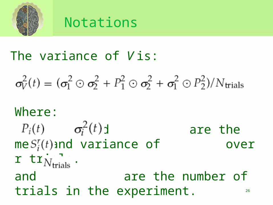
Notations
The variance of V is:
Where:
and are the mean and variance of over r trials.
and are the number of trials in the experiment.
27
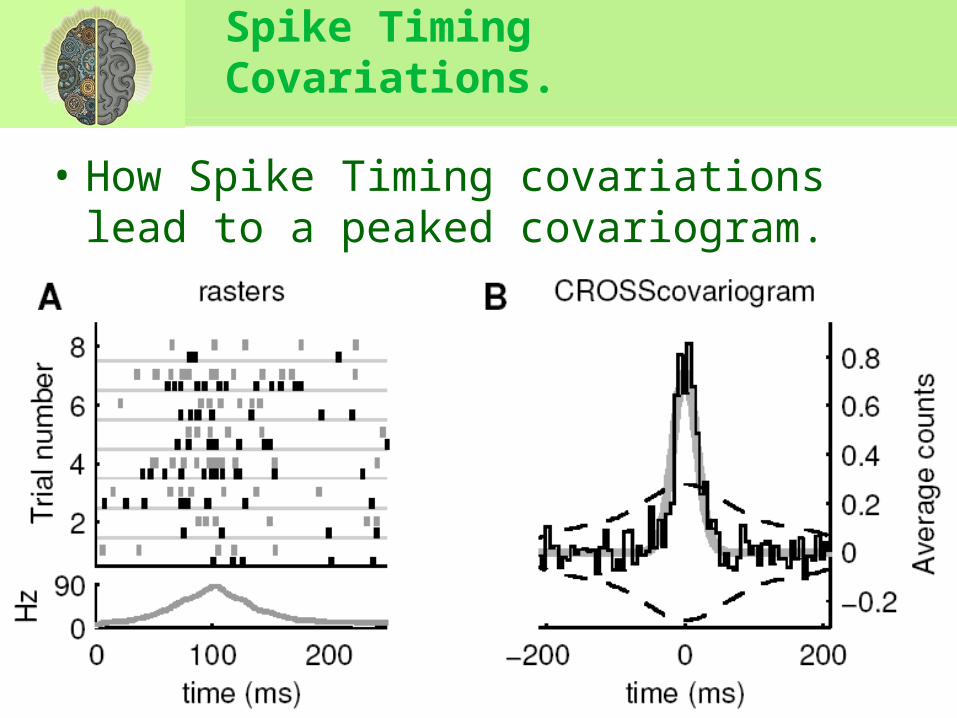
Spike Timing Covariations.
• How Spike Timing covariations lead to a peaked covariogram.
28
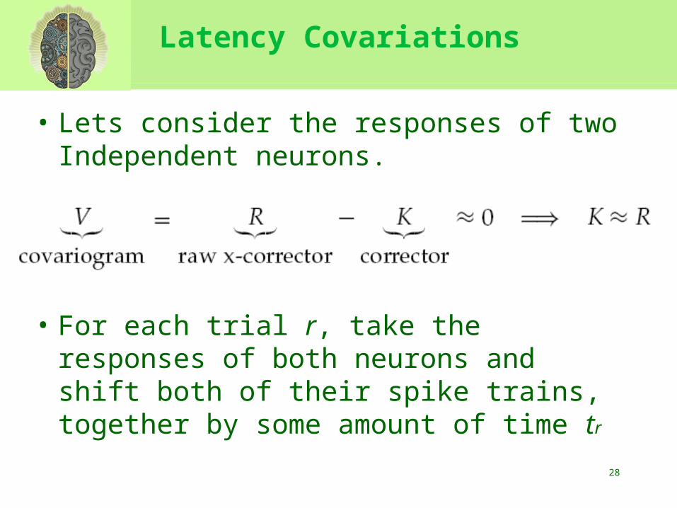
Latency Covariations
• Lets consider the responses of two Independent neurons.
• For each trial r, take the responses of both neurons and shift both of their spike trains, together by some amount of time tr
29
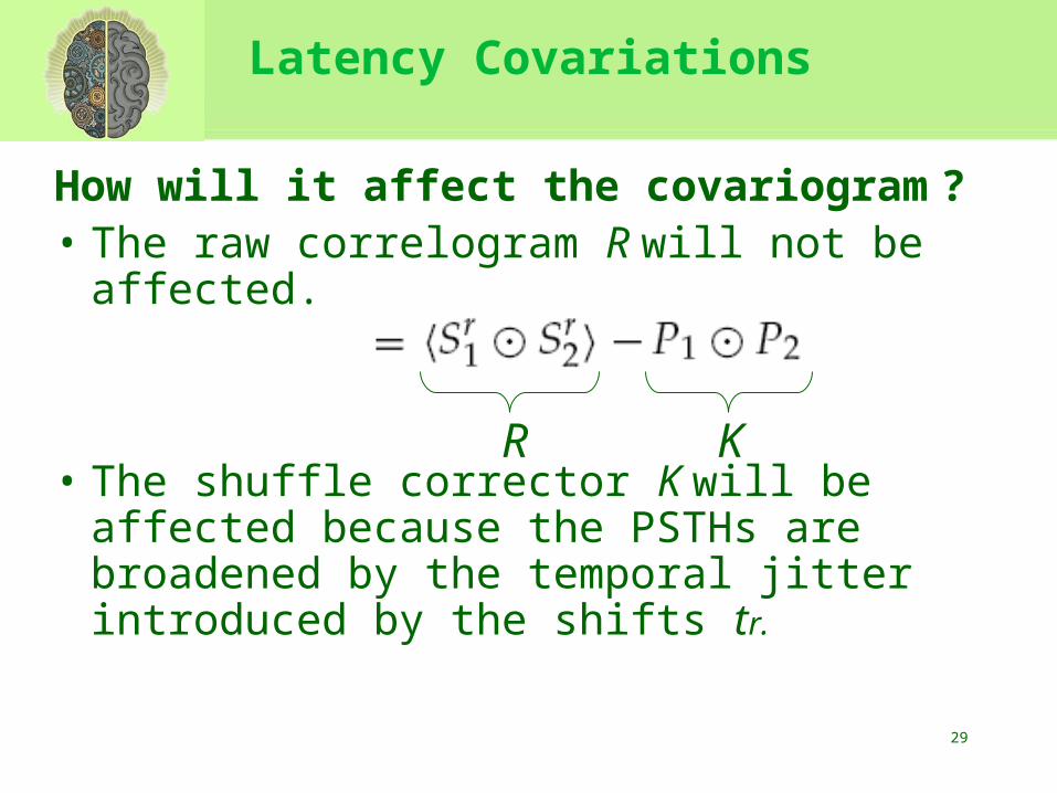
Latency Covariations
How will it affect the covariogram ?• The raw correlogram R will not be
affected.
• The shuffle corrector K will be affected because the PSTHs are broadened by the temporal jitter introduced by the shifts tr.
R K
30
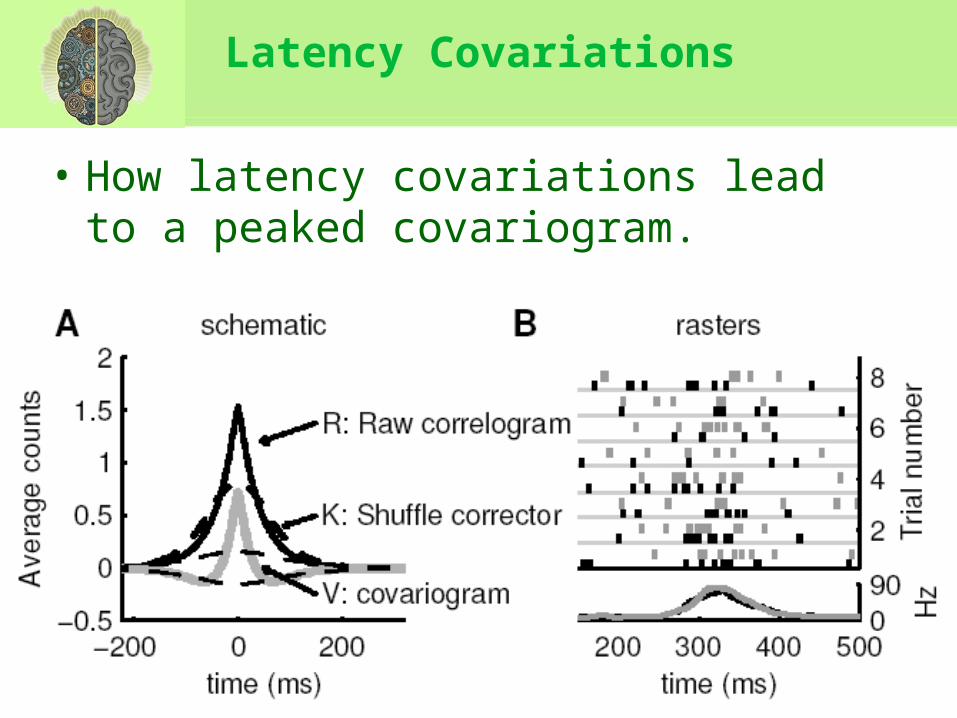
Latency Covariations
• The latency shifts will make K broader, and therefore shallower, while having no effect on R.
• The width and shape of the peak in V are largely determined by the width and shape of the peak in R.
31
Latency Covariations
• How latency covariations lead to a peaked covariogram.
32
Excitability Covariations
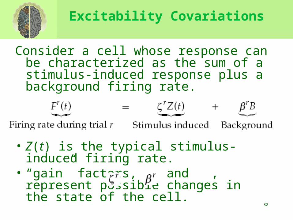
Consider a cell whose response can be characterized as the sum of a stimulus-induced response plus a background firing rate.
• Z(t) is the typical stimulus-induced firing rate.
• “gain” factors, and , represent possible changes in the state of the cell.
33
Excitability Covariations
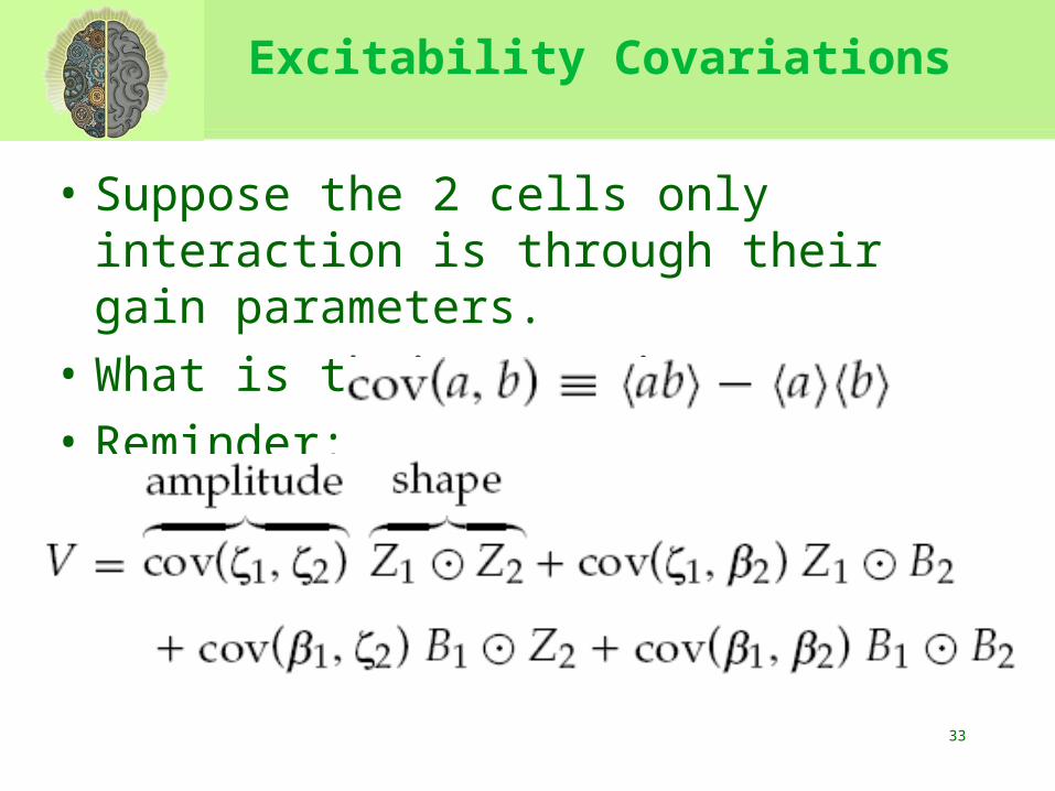
• Suppose the 2 cells only interaction is through their gain parameters.
• What is their covariogram ?
• Reminder:
34
Excitability Covariations
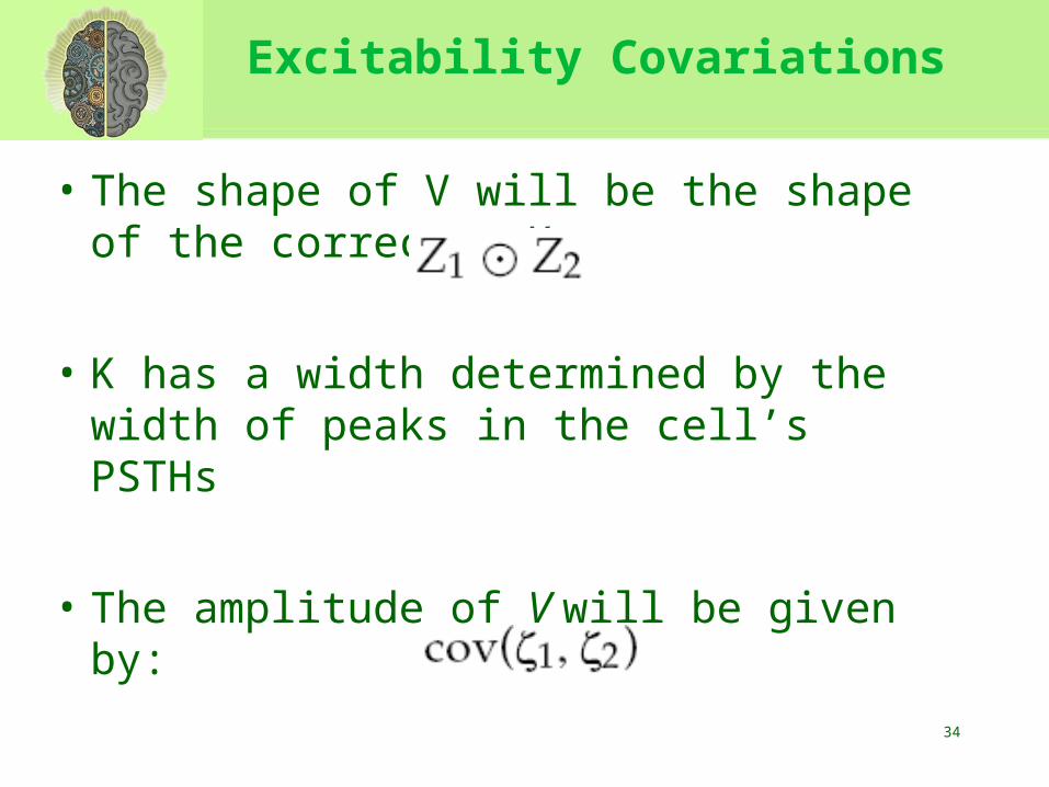
• The shape of V will be the shape of the corrector K:
• K has a width determined by the width of peaks in the cell’s PSTHs
• The amplitude of V will be given by:
35
Excitability Covariations
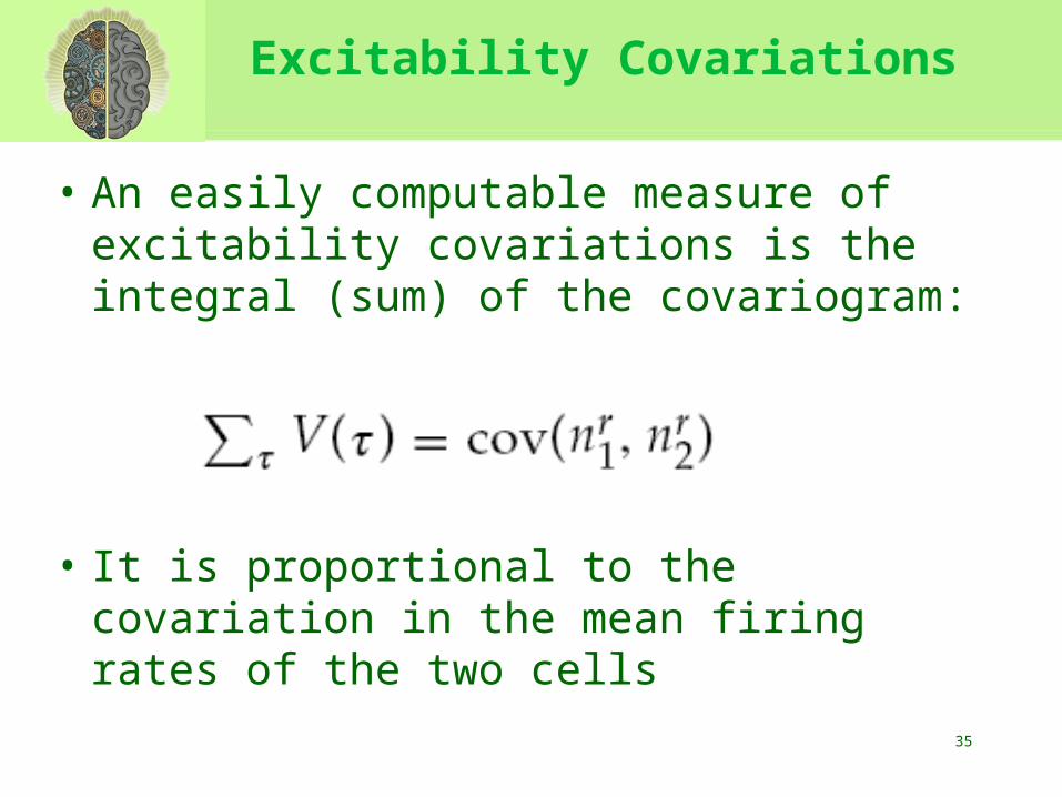
• An easily computable measure of excitability covariations is the integral (sum) of the covariogram:
• It is proportional to the covariation in the mean firing rates of the two cells
36
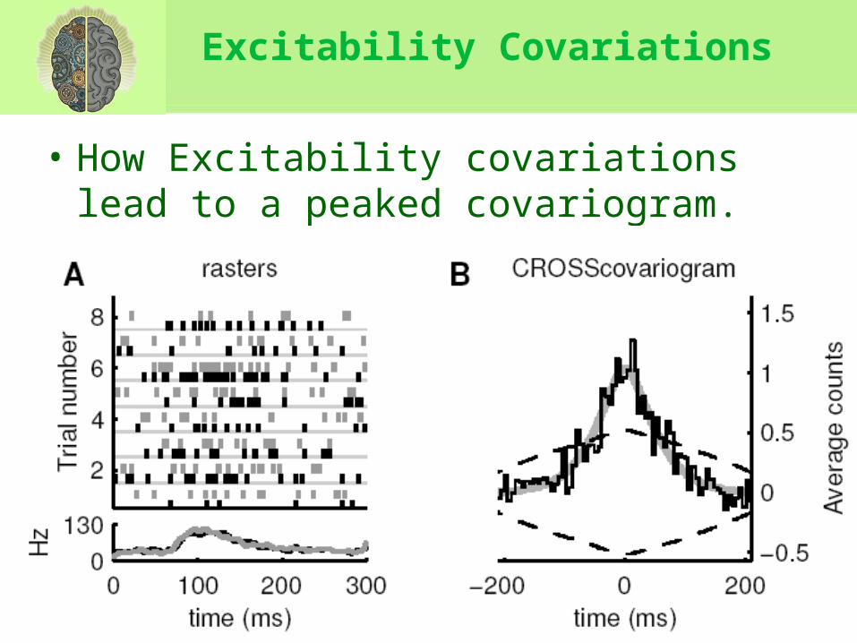
Excitability Covariations
• How Excitability covariations lead to a peaked covariogram.
37
Rules of Thumb
• There are three major points in comparison to latency and excitability covariations:
– Autocovariograms
– Covariogram shapes
– Covariogram integrals
38
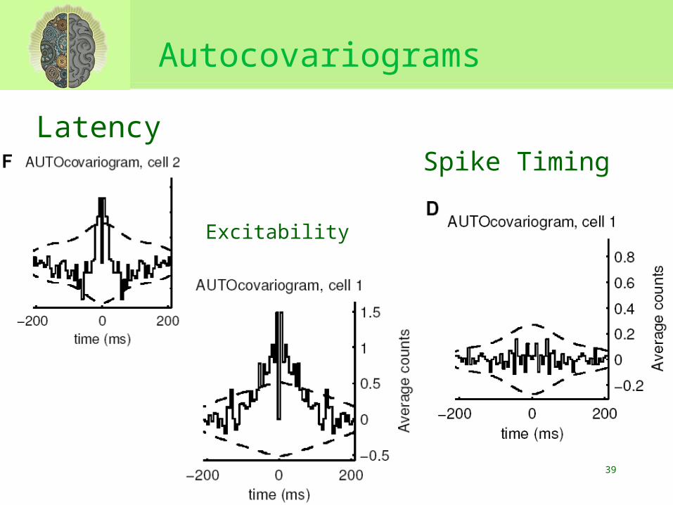
Autocovariograms
• Autocovariograms: This function lets you discern the fine time structure, if any, in the spike train of a single neuron
• Spike Timing autocovariograms are flat and not at all similar to the cross-covariogram. Unlike the ones of Excitability or Latency.
39
Autocovariograms
Latency
Excitability
Spike Timing
40
Covariogram shapes
• Spike timing covariogram shapes are much more arbitrary than Latency or Excitability covariogram shapes.
• Latency and Excitability shapes are tied to the shapes of the PSTHs
• Spike timing shapes are not.
41
covariogram integrals
• Large, positive covariogram integrals imply the presence of an excitability covariations component.
• In the spike timing case, the integral, if positive, will often be small.
42
conclusion
• We want to analyze neuron synchronization by sampling only a small number of trials.
• This is a special case of a more general problem:
Taking the mean of a distribution as representative of all the points of the distribution.
43
conclusion
• For this to work: std << mean
• This is common to gene networks, text searches, network motifs.
• Investigators must interpret means with care !

44
The End
Questions ?
Thank you for listening.