1

Controlled Support MEG Imaging

Srikantan Nagarajan1∗, Oleg Portniaguine2,

Dosik Hwang2, Chris Johnson2 and Kensuke Sekihara3

1Biomagnetic Imaging Laboratory, Department of Radiology, University of California at San Francisco, San

Francisco, CA 94122, USA2Scientific Computing and Imaging Institute, School of Computing, University of Utah, Salt Lake City, UT

841083Department of Electronic Systems and Engineering,Tokyo Metropolitan Institute of Technology,

Asahigaoka 6-6, Hino, Tokyo 191-0065, Japan, USA

* Corresponding author: sri@radiology.ucsf.edu

Abstract

In this paper, we present a novel approach to imaging of sparse and focal neural current

sources from MEG (magnetoencephalography) data. Using the framework of Tikhonov reg-

ularization theory, we introduce a new stabilizer that uses the concept of controlled support

to incorporate a priori assumptions about the area occupied by the focal sources. The pa-

per discusses the underlying Tikhonov theory and its relationship to a Bayesian formulation

which in turn allows us to interpret and better understand other related algorithms.

* Manuscript

2

I. Introduction

The brain’s neuronal activity generates weak magnetic fields (10 fT- 1 pT). Magne-

toenchephalography (MEG) is an non-invasive technique for characterizing these magnetic

fields using an array of superconducting quantum interference devices (SQUIDS). SQUID

magnetometers can measure the changes in the brain’s magnetic field on a millisecond time-

scale, thus, providing unique insights into the dynamic aspects of the brain’s activity. The

goal of biomagnetic imaging is to use MEG data to characterize macroscopic dynamic neural

information by solving an electromagnetic source localization problem.

In the past decade, the development of source localization algorithms has significantly

progressed [1]. Currently, there are two general approaches to estimating MEG sources:

parametric methods and tomographic imaging methods [2]. With parametric methods, a

few current dipoles of uknown location and moment represent the sources. In this case,

the inverse problem is a non-linear optimization in which one estimates the position and

magnitude of the dipoles.

In this paper, we use the tomographic imaging method, where a grid of small voxels repre-

sents entire brain volume. The inverse problem then seeks to recover a whole brain activation

image, represented by the moments and magnitudes of elementary dipolar sources located

at each voxel. The advantage of such a formulation is that the forward problem becomes lin-

ear. However, the ill-posed nature of the imaging problem constitutes considerable difficulty,

most notably due to the non-uniqueness of the solution.

A common way to constrain the non-uniqueness is to use the weighted minimum norm

methods. Such methods find solutions that match the data while minimizing a weighted l2

norm of the solution [2] [3] [4], [5]. Unfortunately, these techniques tend to “smear” focal

sources over the entire reconstruction region.

There are three basic approaches for creating less smeared solutions to the MEG focal

imaging problem: 1) use of lp norms, 2) Bayesian estimation procedures with sparse priors,

and 3) iterative reweighting methods. The first approach that produces sparse solutions uses

an l1, or an lp norm. Although, the l1 norm solution can be formulated as a linear program-

ming problem which converges to the global solution, other lp norm methods are calculated

3

using multidimensional iterative methods which often do not converge to the correct solu-

tion. Furthermore, all lp methods are sensitive to noise [6] [7]. The second approach that

performs better than the first one, is a Bayesian framework with sparse priors derived from

Gibbs distributions [8]. However, these methods are very computationally intensive since full

a posteriori estimation is solved using the Markov-chain Monte-Carlo or mean-field approx-

imation methods [9], [10], [11]. The third approach is iterative reweighted minimum norm

method. The method uses a weighting matrix which, as the iterations proceed, reinforces

strong sources and reduces weak ones [12] [13]. The problems associated with this method

are sensitivity to noise, high dependency on the initial estimate and tendency to accentuate

the peaks of the previous iteration. In addition, the method often produces an image of a

focal source as a scatterred cloud of multiple sources that exist near each other.

In this paper, we combine features of all three approaches outlined above and derive a

novel Controlled Support MEG imaging algorithm, using Tikhonov regularization theory.

The advantages of our algorithm are the quality of focal source images as well as robustness

and speed. In Section II of this paper, we formulate the MEG inverse problem under the

framework of Tikhonov regularization theory, and introduce a way to constrain the problem

using specially selected stabilizing functionals. We then describe the relationship of this for-

mulation to the minimum-norm methods and Bayesian methods. In Section III, we revisit

minimum support stabilizing functional which obtains the sparsest possible solutions, but

may produce an image of a focal source as a cloud of points. To remedy this problem, in

Section IV we derive a new Controlled Support functional, by adding an extra constraining

term to the Minimum Support functional. In Section V, we will explain details of computa-

tionally efficient method of reweighted optimization. Section VI explains how the numerical

minimization is carried out. In Section VI, we demonstate performance of the algorithm us-

ing results from Monte-Carlo simulation studies with realistic sensor geometries and variety

of noise levels.

II. Formulation of the MEG inverse problem using Tikhonov regularization

Let the three Cartesian coordinates of the current dipole strength for each one of the

4

Ns/3 voxels be denoted by the length Ns vector s.. The data consists of a vector b that

contains magnetic field measurements at all receivers. The length of the b is determined by

the number of sensor sites, as denoted by Nb. The forward modeling operator L connects

the model to the data:

Ls = b, (1)

where L is also known as the “lead field.” The lead field is a matrix of size Nb × Ns

that connects the spatial distribution of the dipoles s to measurements at the sensors b.

According to Hadamard [14], the three difficulties in an inverse problem are: 1) the solution

of the inverse problem may not exist, 2) the solution may be non-unique, 3) the solution

may be unstable. The Tikhonov regularization theory resolves these difficulties using the

notions of misfit, the stabilizer and the Tikhonov parametric functional.

The notion of misfit minimization resolves the first difficulty, the non-existence of the

solution. In the event that an exact solution does not exist, we search for the solution

that fits the data approximately, using the misfit functional as a goodness-of-fit measure.

Following the tradition [15], we use a quadratic form of the misfit functional, denoted as φ:

φ(s) = ‖Ls− b‖2/‖b‖2. (2)

When the model produces a misfit that is smaller than the noise level, (Tikhonov discrep-

ancy principle), this model could be a solution of the problem.

The second difficulty, the non-uniqueness, is a situation where many different models have

misfits smaller than the noise level. All of these models could be solutions of the problem.

In practice, we need only one solution that is good. The stabilizing functional, denoted S(s),

measures goodness of the solution. Designing the stabilizer S is a difficult task which we will

discuss in detail in the next two sections. In simplest terms, S is small for “good” models

and large for “bad” models. Therefore, the weighted sum of misfit and stabilizer (denoted

as P ) measures both the goodness of data fit and goodness of the model:

P (s) = φ(s) + λS(s), (3)

where λ is regularization parameter and P is Tikhonov parametric functional. Both dif-

ficulties considered so far, (non-uniqueness and non-existence), are resolved by posing the

5

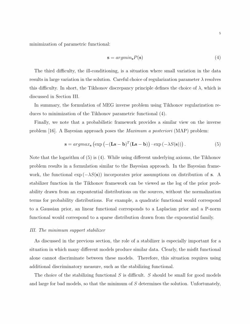
minimization of parametric functional:

s = argminsP (s) (4)

The third difficulty, the ill-conditioning, is a situation where small variation in the data

results in large variation in the solution. Careful choice of regularization parameter λ resolves

this difficulty. In short, the Tikhonov discrepancy principle defines the choice of λ, which is

discussed in Section III.

In summary, the formulation of MEG inverse problem using Tikhonov regularization re-

duces to minimization of the Tikhonov parametric functional (4).

Finally, we note that a probabilistic framework provides a similar view on the inverse

problem [16]. A Bayesian approach poses the Maximum a posteriori (MAP) problem:

s = argmaxs

(exp

(−(Ls− b)T (Ls− b)

)· exp (−λS(s))

). (5)

Note that the logarithm of (5) is (4). While using different underlying axioms, the Tikhonov

problem results in a formulation similar to the Bayesian approach. In the Bayesian frame-

work, the functional exp (−λS(s)) incorporates prior assumptions on distribution of s. A

stabilizer function in the Tikhonov framework can be viewed as the log of the prior prob-

ability drawn from an expontential distributions on the sources, without the normalization

terms for probability distributions. For example, a quadratic functional would correspond

to a Gaussian prior, an linear functional corresponds to a Laplacian prior and a P-norm

functional would correspond to a sparse distribution drawn from the exponential family.

III. The minimum support stabilizer

As discussed in the previous section, the role of a stabilizer is especially important for a

situation in which many different models produce similar data. Clearly, the misfit functional

alone cannot discriminate between these models. Therefore, this situation requires using

additional discriminatory measure, such as the stabilizing functional.

The choice of the stabilizing functional S is difficult. S should be small for good models

and large for bad models, so that the minimum of S determines the solution. Unfortunately,

6

the definition of a good model relies upon empiricial knowledge and depends upon each

particular problem.

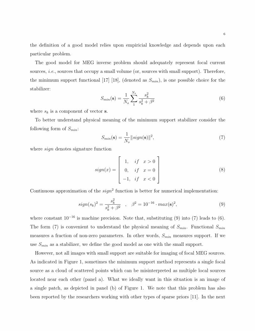
The good model for MEG inverse problem should adequately represent focal current

sources, i.e., sources that occupy a small volume (or, sources with small support). Therefore,

the minimum support functional [17] [18], (denoted as Smin), is one possible choice for the

stabilizer:

Smin(s) =1

Ns

Ns∑1

s2k

s2k + β2

(6)

where sk is a component of vector s.

To better understand physical meaning of the minimum support stabilizer consider the

following form of Smin:

Smin(s) =1

Ns

‖sign(s)‖2, (7)

where sign denotes signature function

sign(x) =

1, if x > 0

0, if x = 0

−1, if x < 0

(8)

Continuous approximation of the sign2 function is better for numerical implementation:

sign(sk)2 =

s2k

s2k + β2

, β2 = 10−16 · max(s)2, (9)

where constant 10−16 is machine precision. Note that, substituting (9) into (7) leads to (6).

The form (7) is convenient to understand the physical meaning of Smin. Functional Smin

measures a fraction of non-zero parameters. In other words, Smin measures support. If we

use Smin as a stabilizer, we define the good model as one with the small support.

However, not all images with small support are suitable for imaging of focal MEG sources.

As indicated in Figure 1, sometimes the minimum support method represents a single focal

source as a cloud of scattered points which can be misinterpreted as multiple local sources

located near each other (panel a). What we ideally want in this situation is an image of

a single patch, as depicted in panel (b) of Figure 1. We note that this problem has also

been reported by the researchers working with other types of sparse priors [11]. In the next

7

section, we deal with this problem by introducing additional restrictive term to the minimum

support stabilizer.

IV. Controlled support stabilizer

The controlled support stabilizer (denoted as Scon) is a functional that reaches its minimum

for images with a predetermined support value α. That value should be small, but not

so small that it creates the undesirable of producing scatterred sources. In other words,

the image in Figure 1 case b, which we consider to be good, produces a minimum of the

stabilizer Scon. The undesirable (scattered) image (case a in the same Figure) corresponds

to a larger value of stabilizer Scon. This discriminative effect of Scon happens because Scon

is a weighted sum of the previously introduced minimum support stabilizer Smin and an

additional restricting term Sreg:

Scon(s) = (1 − α) · Smin(s) + α · Sreg(s), (10)

where the restricting term Sreg is:

Sreg(s) =1

max|s|∑Ns

k=1 |sk|

Ns∑k=1

s2k =

‖s‖2l2

‖s‖l∞‖s‖l1

. (11)

Upon examining expression (11) we notice that the functional Sreg has opposing properties

to Smin, Sreg has a maximum where Smin has a minimum. Obviously, the choice of the

weighting factor α determines the balance between terms (1−α)Smin and αSreg. In summary,

Smin favors minimum support solutions, Sreg favors solutions with large support, and Scon

favors solutions with support controlled by the value of α.

The remainder of this section addresses two important details. First, we must explain why

the effect of Sreg is opposite to that of Smin. Second, we will discuss the normalizations of

Smin and Sreg, which leads to their invariance to discretization. We must note that Sreg is

the square of the l2 norm weighted by the product of l∞ and l1 norms (11). We think of Sreg

as a normalized l2 norm. Therefore, the minimum of Sreg is reached at the minimum l2 norm

solution (a solution with large support where Smin has maximum). The maximum of Smin

is 1, which happens for a case with one non-zero parameter, where Scon is at its minimum.

8

Strictly speaking, the maximum of Sreg is also possible for other cases. However, opposing

properties of the minimums are more important for our purposes.

Now, we consider the normalizations of Smin and Sreg. Factor 1/Ns normalizes Smin

(6), while divisions by l1 and l∞ norms normalize stabilizer Sreg (11). Normalizations are

important for the meaningful summation of Smin and Sreg in expression (10), because they

make the terms bounded:

0 ≤ Smin ≤ 1 0 ≤ Sreg ≤ 1. (12)

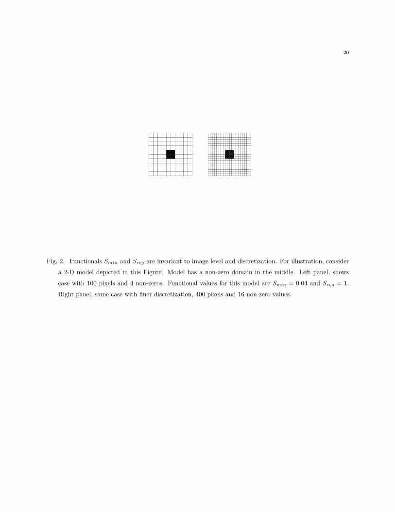
In addition, normalizations make functionals Smin and Sreg invariant to discretization and

grayscale of the image. To illustrate this property, consider an example 2-D image with a

total of 100 pixels, where 96 pixels are zero, and a compact domain in the middle contains 4

pixels – all with the value of a. The left panel in Figure 2 illustrates this case. The following

calculations find values of Smin and Sreg for this case:

Ns = 100,∑Ns

k=1 abs(sk) = 4a, max(s) = a,

∑Ns

k=1 sign(sk)2 = 4,

∑Ns

k=1 s2k = 4a2,

Smin =∑Ns

k=1 sign(sk)2/100 = 0.04

Sreg =∑Ns

k=1(sk)2/(∑Ns

k=1 abs(sk) · max(s))

= 4a2

4a·a = 1

(13)

According to (13), Smin = 0.04 (which is a fraction of the non-zero pixels in the image from

Figure 2) and Sreg = 1. Now, we refine the discretization twice. The resulting image has

total of 400 pixels with 16 pixels containing the value of a, as shown in the right panel of

Figure 2. Calculations similar to (13) show that Smin and Sreg did not change (Smin = 0.04

and Sreg = 1). This example also shows that functional values are invariant to a (image level,

or grayscale). Note that the same properties hold true for 3-D grids and volume models that

we consider in this paper.

9

V. The method of reweighted optimization

In this section, we discuss how to solve minimization problem using the method of reweighted

optimization. To obtain the final form of the objective functional (denoted as Pcon), we sub-

stitute definitions (2) (6) (10) (11) into (3):

Pcon =‖Ls− b‖2

‖b‖2+ λ

(1 − α

Ns

Ns∑k=1

s2k

s2k + β2

+α

‖s‖l∞ · ‖s‖l1

Ns∑k=1

s2k

). (14)

In this section, we discuss the idea of how to solve the minimization problem:

s = argminsPcon(s). (15)

Arguably, the minimization of Pcon is difficult, because it is a non-linear (non-quadratic)

functional of s. We have two feasible options for the numerical solution of our non-quadratic

problem. The first uses gradient-type inversion methods, and the second uses the method

of reweighted optimization. While the gradient-type minimization method is well known

[19], this method requires computing the gradient of a functional (14). Computing such a

gradient is problematic since we previously used sign while constructing Pcon (see formulas

(8) and (9)).

In this paper, we use the method of reweighted optimization, a historical choice for related

minimum-support problem [17], [18], [20]. In addition, a number of researchers have found

the reweighted optimization convenient [21] [22], [23], especially for cases where non-linearity

is represented by weights to the quadratic term. This is exactly our case. Notice that the

term s2k in (14) can be taken out of the brackets

Pcon =‖Ls− b‖2

‖b‖2+ λ

Ns∑k=1

(1 − α

Ns

1

s2k + β2

+α

‖s‖l∞ · ‖s‖l1

)s2

k. (16)

Thus, model-dependent weighting of the quadratic functional represents the non-linearity in

(14):

Pcon =‖Ls− b‖2

‖b‖+ λ

Ns∑k=1

w−2k · s2

k, (17)

where wk is model-dependent weight

w−2k =

1 − α

Ns

1

s2k + β2

+α

‖s‖l∞ · ‖s‖l1

. (18)

10

It is convenient to assemble weights into a sparse diagonal matrix W(s) with terms wk in

the main diagonal, and write (17) in matrix notations:

Pcon =‖Ls− b‖2

‖b‖2+ λ‖W(s)−1s‖2 (19)

To understand our optimization algorithm in detail, it is necessary to convert the parametric

functional to a purely quadratic form, which has a known analytic solution. This form is

obtained by transforming the problem into a space of weighted model parameters. To do

that, we insert W(s)W(s)−1 term into (19):

Pcon =‖LW(s)W(s)−1s− b‖2

‖b‖2+ λ‖W(s)−1s‖2. (20)

Then, we transform (20) by replacing the variables:

s = W(s)sw, Lw = LW(s). (21)

After substituting (21), expression (20) results in a purely quadratic form of the functional

with respect to sw:

P (sw) =‖Lwsw − b‖2

‖b‖2+ λ‖sw‖2. (22)

Since Pcon(sw) is purely quadratic with respect to sw, the minimization problem for Pcon(sw)

has an analytical solution, known as the Riesz representation theorem [24]:

sw = LTw(LwLT

w + λ‖b‖2Ib)−1b, (23)

where Ib is unit matrix in the space of data (of size Nb × Nb).

Thus, the idea of reweighted optimization is to solve (15) iteratively, assuming the weights

are constant on each iteration. Starting from the initial guess for the weights, we can use

the Riesz representation theorem to find weighted solution. We can then convert back to

original space, update the weights depending on the solution, and repeat the iterative process.

The next section discusses the details of this process. The above equation is identical to

the MAP estimator with Gaussian priors for the sources and the noise, where the source

variance is assumed to be an unknown diagonal matrix and the noise variance is known and

parameterized by λ.

11

VI. The minimization algorithm

The algorithm for minimizing a parametric functional is iterative. On each iteration,

(enumerated with index n), we compute the updates of: the weights Wn, the weighted lead

fields Lwn, the weighted model swn, and the update of the model sn. These quantities depend

upon values from previous iteration (denoted with index n − 1). Inputs to the algorithm

include the data b, noise level estimate φ0, as well as the support parameter α. Before the

first iteration, we precompute the lead fields L, set weights to one W0 = Is, and set the

current model update to zero s0 = 0. The important additional step are incorporated in the

final algorithm. The first is the choice of regularization parameter, the second is the line

search correction, and the third is termination criterion.

According to Tikhonov condition, the choice of the regularization parameter λ should be

such that the misfit (2) at the solution equals an a priori known noise level φ0 [25],:

‖Lwsw − b‖2

‖b‖2= φ0. (24)

Substituting (23) into (24) yields the equation

‖LwnLwTn (LwnLw

Tn + λ‖b‖Ib)−1b− b‖2 = φ0‖b‖2 (25)

which we solve with a fixed point iteration method. In equation (25) the only unknown

variable is the scalar parameter λ. Since the Gramm matrix LwnLwTn is small (Nb × Nb,

where Nb is small), the fixed point iteration method easily solves equation (25) for λ. For

the cases where the data dimension Nb is large, which makes the direct inversion of a Gramm

matrix impractical, solving equation (22) using the Riesz theorem (23) can be substituted

by solving (22) via a conjugate gradient method [20]. In this paper, we consider processing

of MEG data from an array of 102 sensors, so the dimension of data is small Nb = 102

and therefore the Gramm matrix is easily invertible with direct methods. Such a choice

of the regularization term is analagous to setting the noise variance in the Bayesian MAP

estimation procedure.

Second, to ensure convergence of the algorithm, we incorporate a line search procedure.

Convergence of the reweighted optimization depends upon how accurately the equation (22)

12

approximates the original non-quadratic equation (19). That, in turn, depends on assump-

tion of constant weights, which, in our case, are dependent on s. The usual assumption for

any iterative method is that the changes in a model are small from one iteration sn−1 to

the next sn. That assumption may not always hold, and therefore, steps which converge on

equation (22) may be divergent on the original equation (16) due to significant changes in

W(s). The well known method of line search [19] serves to correct this problem. Once the

next approximate update s′n is found from the previous update sn−1 using the approximate

formula (22), we check the value of original non-linear objective functional Pcon(s′n). If the

objective functional decreases, the line search is not deployed. If the objective functional

increases, (which signifies the divergent step), we perform a line search.

If Pcon(sn−1) < Pcon(sn), we perform a line search, by searching for the minimum of Pcon

with respect to the scalar variable t (the step length):

t = argmintPcon(sn−1 + t(s′n − sn − 1))

If Pcon(sn−1) > Pcon(sn), then we set t = 1 and do not perform the line search. Note that the

smaller step size t is, the closer the corrected update sn is to the previous update sn−1 from

which the weights Wn were derived. Thus, the smaller t is the less weights change from n−1

iteration to n, and therefore, our quadratic approximation becomes more accurate. With

small enough t, a smaller value of Pcon will always be found somewhere between sn−1 and s′n.

Minimization of the scalar functional Pcon with respect to scalar argument t is a simple 1-D

problem. That problem is solved by sampling the function at a few points (usually three or

four), fitting the parabola into it, and finding the argument of a minimum. Such sampling

is fast, for one estimate of the functional we only need to solve one forward problem. In

many previously conducted studies with minimum support functional Smin, the reweighted

optimization has never diverged [17] [18]. Our new controlled support functional, Scon, is

dominated by term Smin. Therefore, we expected the same good convergence for S as was

reported for Smin. However, in the Monte-Carlo simulations carried out in this paper and

with some limited datasets, the algorithm has never called the line search routine because

the divergence was never detected.

Third, the termination criterion was formulated based on the following two observations.

13

First, we must observe that all updates sn produce the same misfit φ0 (due to enforcement

of the Tikhonov condition). Therefore, only the second term Scon determines the minimum

of Pcon(sn) on a given set of arguments sn. This second term consists of two parts: (1 −

α)Smin(sn), and αSreg(sn). The second observation is that the Smin(sn) term decreases with

n, and the Sreg(sn) term increases with n. This happens because on the first iteration n = 1

we produce the minimum norm solution, and then progress towards more focused solutions

(see discussion about opposing properties of Smin and Sreg in section III). So, the dominance

of αSreg term over (1 − α)Smin term signifies close proximity to the minimum of Pcon.

We summarize the complete algorithm as follows:

1. Compute Lwn using (21)

Lwn = LWn−1.

2. Determine regularization parameter by fixed point iteration of equation (25).

3. Find the weighted model swn using (23):

swn = LwTn (LwnLw

Tn + λ‖b‖Ib)−1b.

4. Find preliminary update of the model sn using (21),

s′n = Wn−1swn.

5. Check for divergence and incorporate line search.

6. Corrected update sn is found from the previous update sn−1 using step length t:

sn = sn−1 + l(s′n − sn−1).

7. Check for termination criterion. We stop iterations if

(1 − α)Smin(sn) < αSreg(sn).

8. Find the updated weight Wn using (18). and go to Step 1, repeating all steps in the loop.

VII. Results and Discussion

14

In simulations we demonstrate the algorithm performance, estimate localization accuracy

and speed of the method. The geometry for all simulations were from an MR (Magnetic

Resonance) image of a subject. Figure 3 shows a head surface extracted from the MR volume

image. We transformed the MEG sensor array to MRI coordinates by matching the reference

points (measured on the subject’s head) and the extracted head surface [26]. Figure 3 shows

the MEG array as a “helmet” consisting of 102 square sensor “plates.” Each plate has

magnetic coils that measure the normal (to the plate) component of the magnetic field. The

middle of the plate serves as a reference point. In order to parameterize the inverse problem,

we divided the volume of the brain into 30,000 cubic voxels of size 4 × 4 × 4 millimeters.

Vector s consists of strengths of three components of current dipoles within each voxel. This

produces Ns = 90, 000 free inversion parameters (unknowns). This parameterization takes

into account both gray matter and white brain matter. We did not use the alternative

parameterization with the cortical surface constraint because the final reconstruction result

would strongly depend on the accuracy of the cortical surface extraction procedure. The

controlled support algorithm is the point of our investigation. So, we did not use cortical

surface extraction since it may mask the evaluation of the algorithm’s performance.

We built the underlying forward model (lead field operator) using the formula for a dipole

in a homogeneous sphere [3] We computed the sensitivity kernel for each sensor (a row of

matrix L), using an individual sphere locally fit to the surface of the head near that particular

sensor site [27].

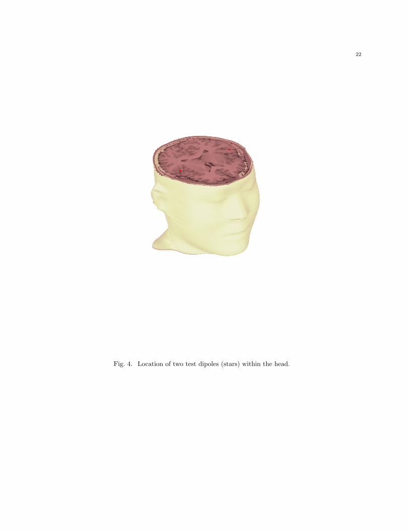
As a first numerical experiment, we placed two dipoles within the brain, approximately

at the level of the primary auditory cortex. Figure 4 shows the location of dipoles within

the brain. That setup defines the vector s as zeros everywhere except the specified dipole

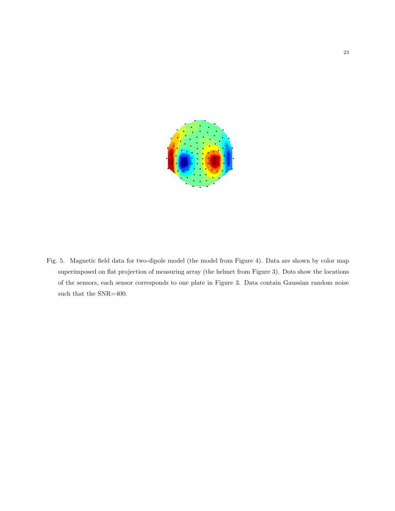
locations. We generate the data b using the forward equation (1), adding Gaussian random

noise such that the SNR is 400. The level of noise is set relative to the data and measured

in the same units as a normalized misfit, as defined by the formula

bnoise = b + n‖b‖

‖n‖ · SNR(26)

where SNR is the signal-to-noise ratio defined by the ratio of the average signal power across

channels divided by the average noise power, and n is the noise vector. Figure 5 shows the

15

resulting data as a flat projection.

To illustrate convergence, Figure 6 shows the evolution of stabilizers during iterations, and

Figure 7 shows the evolution of the solution. The isolines in Figure 7 display the magnitudes

of the dipoles in the solutions, superimposed on a corresponding MRI slice.

Figure 7 displays six solutions produced on each iteration. The first solution (Panel 1) is

a minimum norm solution that is smooth, and maximums are far away from the true dipole

locations. In contrast to a common misconception about reweighted optimization methods,

observe how the location of maximum activation shifts during reweighted iterations (Panels

1-6 in Figure 7). Note that the method discussed here does not simply accentuate the peaks

of the previous iteration. The size and shape of the estimated source area are mainly due to

the model and the noise level and do not directly relate to the size and shape of the orignal

source.

Each of these solutions describe the data equally well, but they do not describe the prior

expectations that the activity is focused. The solutions are indistinguishable in terms of the

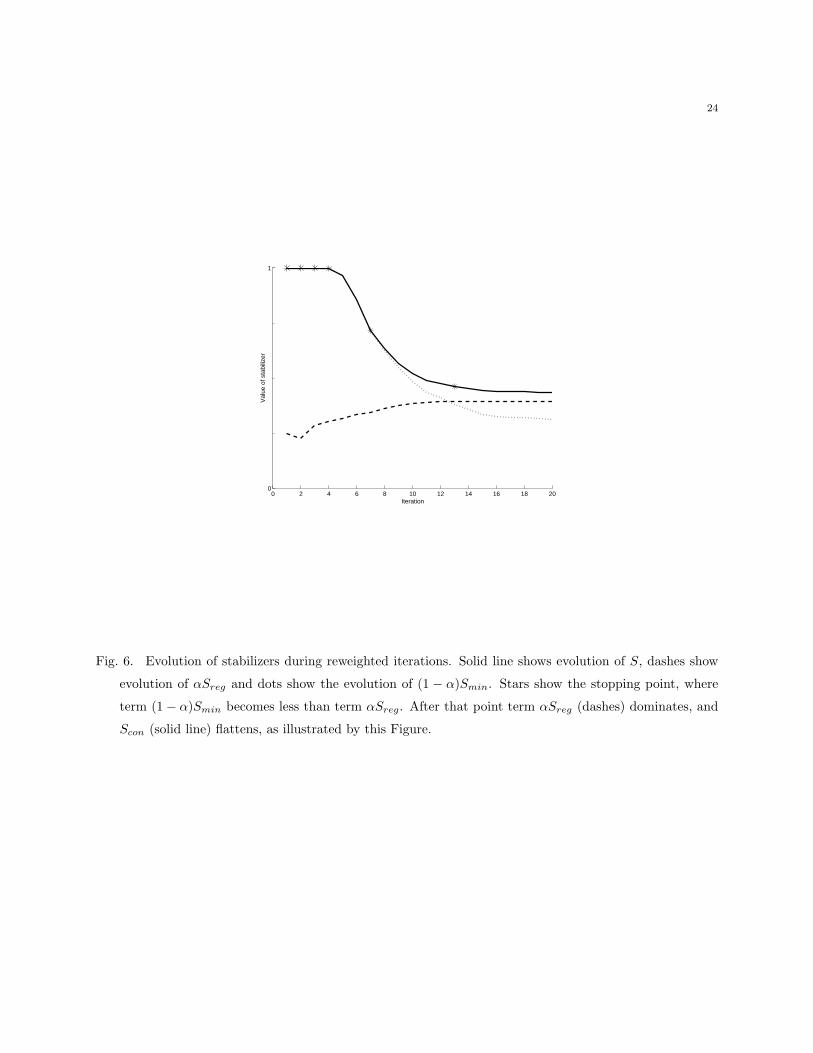
data fit, however, they have different values of the stabilizer. Figure 6 shows evolutions of a

stabilizer S (solid line) and its individual components (α−1)Smin (dots) and αSreg (dashes).

We see that the first solution has a large value of a stabilizer, and on the next iterations, the

stabilizer decreases to a minimum.

We have empirically determined, from our Monte-Carlo experiments, that the best esti-

mate of the dipole location is not the maximum of the image, but rather the location of

the maximum of a local weighted average of the image around its maximum solution. Such

a technique is better since it provides estimates located away from the grid nodes, and is,

therefore, less sensitive to a given inversion grid. We estimate the dipole locations by thresh-

olding the whole image at 10% to the maximum, separating the individual maximums by

clustering, and determining the center of each cluster as the average of a position of cluster

points with weights corresponding to the intensity of the image. This procedure is very fast

for our compact images (fractions of a second) and does not increase the overall computation

time.

Second, we estimate the localization accuracy and speed of our algorithm using the Monte-

16

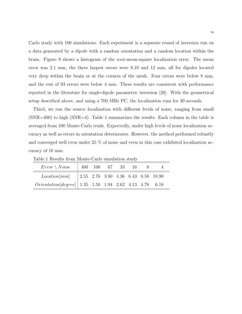
Carlo study with 100 simulations. Each experiment is a separate round of inversion run on

a data generated by a dipole with a random orientation and a random location within the

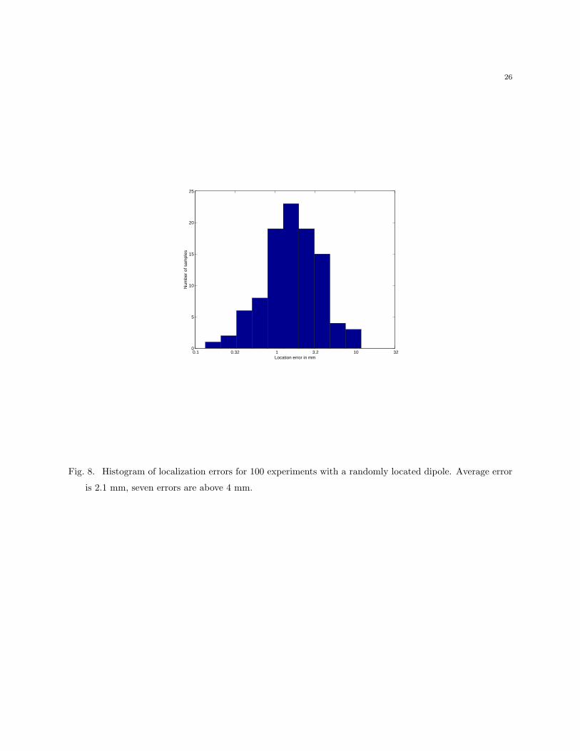
brain. Figure 8 shows a histogram of the root-mean-square localization error. The mean

error was 2.1 mm, the three largest errors were 8,10 and 12 mm, all for dipoles located

very deep within the brain or at the corners of the mesh. Four errors were below 8 mm,

and the rest of 93 errors were below 4 mm. These results are consistent with performance

reported in the literature for single-dipole parametric inversion [28]. With the geometrical

setup described above, and using a 700 MHz PC, the localization runs for 30 seconds.

Third, we run the source localization with different levels of noise, ranging from small

(SNR=400) to high (SNR=4). Table 1 summarizes the results. Each column in the table is

averaged from 100 Monte-Carlo trials. Expectedly, under high levels of noise localization ac-

curacy as well as errors in orientation deteriorates. However, the method performed robustly

and converged well even under 25 % of noise and even in this case exhibited localization ac-

curacy of 10 mm.

Table.1 Results from Monte-Carlo simulation study

Error \ Noise 400 100 67 33 16 8 4

Location[mm] 2.55 2.76 3.80 4.36 6.43 8.58 10.90

Orientation[degree] 1.35 1.50 1.94 2.62 4.13 4.78 6.18

17

Acknowledgements

This work was partially supported under NIH grant P41 RR12553-03 and also by grants

from the Whitaker Foundation and NIH (R01DC004855) to SN. The authors would like

to thank Dr. M. Funke from the University of Utah Department of Radiology for his help

providing the realistic MEG array geometry and Blythe Nobleman from Scientific Computing

and Imaging Institute at the University of Utah, for her many useful suggestions pertaining

to the manuscript.

References

[1] S. Baillet, J.C. Mosher, and R.M. Leahy. Mapping human brain function using intrinsic electromagnetic signals.

IEEE Signal Processing Magazine, in press, 2001.

[2] M. Hamalainen, R. Hari, R.J. Ilmoniemi, J. Knuutila, and O.V. Lounasmaa. Magnetoencephalography - theory,

instrumentation, and applications to noninvasive studies of the working braing. Reviews in Modern Physics,

65:413–497, 1993.

[3] J. Sarvas. Basic mathematical and electromagnetic concepts of the biomagnetic inverse problem. Phys. Med.

Biol., 32:11–22, 1987.

[4] J.Z. Wang, S. J. Williamson, and L. Kaufman. Magnetic source images determined by a lead-field analysis: the

unique minimum-norm least-squares estimation. IEEE Trans Biomed Eng, 39(7):665–675, 1992.

[5] R. D. Pascual-Marqui and R. Biscay-Lirio. Spatial resolution of neuronal generators based on eeg and meg

measurements. Int J Neurosci, 68(1-2):93–105, 1993.

[6] K. Matsuura and Y. Okabe. Selective minimum-norm solution of the biomagnetic inverse problem. IEEE Trans

Biomed Eng, 42(6):608–615, 1995.

[7] K. Uutela, M. Hamalainen, and E. Somersalo. Visualization of magnetoencephalographic data using minimum

current estimates. Neuroimage, 10(2):173–180, 1999.

[8] D.M. Schmidt, J.S. George, and C.C. Wood. Bayesian inference applied to the electromagnetic inverse problem.

Hum Brain Mapp, 7(3):195–212, 1999.

[9] C. Bertrand, Y. Hamada, and H. Kado. Mri prior computation and parallel tempering algorithm: a probabilistic

resolution of the meg/eeg inverse problem. Brain Topogr, 14(1):57–68, 2001.

[10] C. Bertrand, M. Ohmi, R. Suzuki, and H. Kado. A probabilistic solution to the meg inverse problem via mcmc

methods: the reversible jump and parallel tempering algorithms. IEEE Trans Biomed Eng, 48(5):533–542, 2001.

[11] J.W. Phillips, R. M. Leahy, and J. C. Mosher. Meg-based imaging of focal neuronal current sources. IEEE Trans

Med Imaging, 16(3):338–348, 1997.

[12] I.F. Gorodnitsky and B.D. Rao. Sparse signal reconstruction from limited data using focuss: A recursive weighted

norm minimumization algorithm. IEEE Trans. on Signal Processing, 45:600–616, 1997.

[13] I.F. Gorodnitsky and J.S. George. Neuromagnetic source imaging with focuss: a recursive weighted minimum

norm algorithm. Electroencephalogr Clin Neurophysiol, 95(4):231–51, 1995.

[14] J. Hadamard. Sur les problemes aux derivees parielies et leur signification physique. Bull. Univ. of Princeton,

pages 49–52, 1902. in French.

18

[15] U. Eckhart. Weber’s problem and weiszfeld’s algorithm in general spaces. Math. Programming, 18:186–196,

1980.

[16] S. Baillet and L. Garnero. A bayesian approach to introducing anatomo-functional priors in the eeg/meg inverse

problem. IEEE Trans Biomed Eng, 44(5):374–385, 1997.

[17] B.J. Last and K. Kubik. Compact gravity inversion. Geophysics, 48:713–721, 1983.

[18] O. Portniaguine and M.S. Zhdanov. Focusing geophysical inversion images. Geophysics, 64:874–887, 1999.

[19] R. Fletcher. Practical methods of optimization. Wiley and Sons, 1981.

[20] O. Portniaguine. Image focusing and data compression in the solution of geophysical inverse problems. PhD

thesis, University of Utah, 1999.

[21] R. Wolke and H. Schwetlick. Iteratively reweighted least squares: algorithms, convergence analysis, and numerical

comparisons. SIAM, J. Sci.Stat. Comput., 9:907–921, 1988.

[22] D.P. O’Leary. Robust regression computation using iteratively reweighted least squares. SIAM J. Matrix Anal.

Appl., 11:466–480, 1990.

[23] C. G. Farquharson and D.W. Oldenburg. Non-linear inversion using general measures of data misfit and model

structure. Geophysical Journal International, 134:213–227, 1998.

[24] C.D. Aliprantis and O. Burkinshaw. Locally solid Riesz spaces. Academic Press, New York & London, 1978.

[25] A.N. Tikhonov and Y.V. Arsenin. Solution of ill-posed problems. Winston and Sons, 1977.

[26] D. Kozinska, F. Carducci, and K. Nowinski. Automatic alignment of eeg/meg and mri data sets. Clinical

Neurophysiology, 112:1553–1561, 2001.

[27] M.X. Huang, J.C. Mosher, and R.M. Leahy. A sensor-weighted overlapping-sphere head model and exhaustive

head model comparison for meg. Phys Med Biol, 44(2):423–440, 1999.

[28] R.M. Leahy, J.C. Mosher, M.E. Spencer, M.X. Huang, and J.D. Lewine. A study of dipole localization accuracy

for meg and eeg using a human skull phantom. Electroencephalogr Clin Neurophysiol, 107(2):159–173, 1998.

19

Figures

a) b)

Fig. 1. This Figure illustrates outcomes of two attempts to image a single focal source with two different

stabilizers. a) Image obtained with minimum support stabilizer is a cloud of disconnected multiple focal

sources located near each other. b) Image obtained with controlled support stabilizer is a single patch.

20

Fig. 2. Functionals Smin and Sreg are invariant to image level and discretization. For illustration, consider

a 2-D model depicted in this Figure. Model has a non-zero domain in the middle. Left panel, shows

case with 100 pixels and 4 non-zeros. Functional values for this model are Smin = 0.04 and Sreg = 1.

Right panel, same case with finer discretization, 400 pixels and 16 non-zero values.

21

Fig. 3. Geometry that was used in the model study. An outer head surface was extracted from the subject’s

MRI. MEG sensor array (a ”hat” consisting of square receiver ”plates”, as shown here) was positioned

in MRI coordinates by matching the reference points to the head surface. Each ”plate” measures normal

component of a magnetic field.

22

Fig. 4. Location of two test dipoles (stars) within the head.

23

Fig. 5. Magnetic field data for two-dipole model (the model from Figure 4). Data are shown by color map

superimposed on flat projection of measuring array (the helmet from Figure 3). Dots show the locations

of the sensors, each sensor corresponds to one plate in Figure 3. Data contain Gaussian random noise

such that the SNR=400.

24

0 2 4 6 8 10 12 14 16 18 200

1

Iteration

Val

ue o

f sta

biliz

er

Fig. 6. Evolution of stabilizers during reweighted iterations. Solid line shows evolution of S, dashes show

evolution of αSreg and dots show the evolution of (1 − α)Smin. Stars show the stopping point, where

term (1 − α)Smin becomes less than term αSreg. After that point term αSreg (dashes) dominates, and

Scon (solid line) flattens, as illustrated by this Figure.

25

1

2

3

4

7

13

Fig. 7. Evolution of solution during reweighted iterations. The case corresponds to example discussed in

Figure 6. Stars show ”true” location of dipoles (location of dipoles within the head is shown in Figure

4). Solution is superimposed on corresponding MRI slice as isolines. Panels numbered 1,2,3,4,7,13 show

the solutions at the corresponding iteration.

26

0.1 0.32 1 3.2 10 320

5

10

15

20

25

Location error in mm

Num

ber

of s

ampl

es

Fig. 8. Histogram of localization errors for 100 experiments with a randomly located dipole. Average error

is 2.1 mm, seven errors are above 4 mm.