Embed Size (px)
Citation preview

Comparison of magnetic, electrical and GPR surveys to detect buried forensic objects in 1
semi-urban and domestic patio environments 2
3
Hansen, J.D.* & Pringle, J.K. 4
5
School of Physical Sciences & Geography, Keele University, Keele, Staffs, ST5 5BG, UK. 6
7
*Contact email: [email protected] 8
9
Abstract 10
11
Near-surface geophysical techniques should be routinely utilised by law enforcement agencies to 12
locate shallowly buried forensic objects, saving manpower and resources. However, there has 13
been little published research on optimum geophysical detection method(s) and configurations 14
beyond metal detectors. This paper details multi-technique geophysical surveys to detect 15
simulated unmarked illegal weapons, explosive devices and arms caches that were shallowly 16
buried within a semi-urban environment test site. A concrete patio was then overlaid to represent 17
a common household garden environment before re-surveying. Results showed the easily-18
utilised magnetic susceptibility probe was optimal for target detection in both semi-urban and 19
patio environments, whilst basic metal detector surveys had a lower target detection rate in the 20
patio scenario with some targets remaining undetected. High-frequency (900 MHz) GPR 21
antennae were optimum for target detection in the semi-urban environment whilst 450 and 900 22
MHz frequencies had similar detection rates in the patio scenario. Resistivity surveys at 0.25 m 23
probe and sampling spacing were good for target detection in the semi-urban environment. 2D 24
profiles were sufficient for target detection but resistivity datasets required site detrending to 25
resolve targets in map view. Forensic geophysical techniques are rapidly evolving to assist 26
search investigators to detect hitherto difficult-to-locate buried forensic targets. 27
28
5,832 words, 16 Figures and 2 Tables 29
30
Running title: Semi-urban and patio geophysical surveys 31
32
33
34
35
36
37
38
39
40
41
42
43
44
Introduction 45
46
Geo-scientific methods are being increasingly utilised and reported upon by forensic search teams for the 47
detection and location of clandestinely buried material in terrestrial environments. Parker et al. (2010) 48
provides a comprehensive review of forensic geophysical searches within freshwater bodies. In a law 49
enforcement context, forensic burials are at a maximum of 10 m below ground level (bgl) and usually 50
much shallower (Fenning & Donnelly 2004). Forensic objects needing to be located vary from illegally 51
buried weapons and explosives, landmines and improvised explosive devices (IEDs), drugs and weapons 52
caches to clandestine graves of murder victims and mass genocide graves (see Pringle et al. 2012a). In 53
the U.S.A., neighbourhood criminal gangs often hide used illegal weapons for later recovery (Dionne et 54
al. 2011). 55
56
Recovery of buried forensic material often results in successful criminal convictions and it is thus critical 57
for them to be located (Harrison & Donnelly 2009). Law enforcement agencies need to have prioritised 58
locations to physically excavate due to shortages in manpower and resources, especially if the search area 59
is large. Specialist trained search dogs have been widely used to identify different buried objects, 60
commonly IEDs (see Curran et al. 2010), drugs and human remains, the latter teams sometimes referred 61
to as cadaver dogs (see Rebmann et al. 2000) but are less successful with buried inorganic objects. Metal 62
detector search teams are used during forensic investigations when deemed appropriate, especially when 63
there is a high contrast between the target and local background environment (see Nobes 2000). 64
65
Geotechnical investigations routinely use near-surface geophysical methods to identify buried locations 66
of, for example, cleared building foundations and underground services (see Reynolds, 2011), as well as 67
environmental forensic objects such as illegally buried waste (see Bavusi et al. 2006; Ruffell & Kulessa 68
2009). Magnetic detection methods are commonly used in geotechnical (e.g. Marchetti et al. 2002; 69
Reynolds, 2004; Reynolds 2011) and forensic archaeological investigations (see Linford 2004; Hunter & 70
Cox 2005). Acheroy (2007) provides a useful review of field detection of anti-personnel mines using 71
ground penetrating radar (GPR). 72
73
However, little control study research has been published in which buried forensic objects are detected 74
using a variety of geophysical methods, other than to confirm metal detection team results (e.g. Davenport 75
2001; Rezos et al. 2010) and for human remains (e.g. Miller 1996; Davenport 2001; Schultz et al. 2006, 76
Schultz 2008; Pringle et al. 2008; Pringle et al. 2012b). Dionne et al. (2011) did conduct a control study 77
with buried weapons and found electro-magnetic equipment could detect metallic objects buried in a grid 78
distribution in a rural environment but this study did not have access to a Geonics™ EM38 instrument. 79
The Murphy & Cheetham (2008) control study found that magnetic techniques proved difficult to 80
differentiate between target buried weapons and background materials, even when surface metallic items 81
were cleared from the survey site prior to geophysical data collection. Murphy & Cheetham (2008) also 82
found GPR methods could locate buried forensic targets but were difficult to locate in certain orientations 83
so GPR was an obvious technique to trial. 84
85
This case study therefore intended to utilise a variety of current commercial, shallow near-surface 86
geophysical equipment to locate hard-to-detect, small-scale buried forensic metallic objects in a semi-87
urban environment, using survey procedures commonly used in geotechnical and archaeological 88
investigations. The study site was also re-surveyed once a concrete slab patio was laid to also simulate a 89
common domestic property garden forensic scenario (see Toms et al. 2008; Congram 2008; Billinger 90
2009). To give the study more of a sense of realism, the survey is that of a heterogeneous soil content, 91
representative of a U.K. garden, and both target objects and non-target objects (brick, metallic screw and 92
iron plate) were also buried. The locations and orientations of objects were recorded. 93
94
Study objectives for both semi-urban and patio environments were to: 1) evaluate and find optimum 95
magnetic detection technique(s) of the target buried forensic material; 2) compare with electrical and GPR 96
detection methods; 3) determine optimum GPR detection frequencies; 4) determine optimum respective 97
equipment configuration(s) / survey specifications / optimum processing steps; 5) determine which 98
technique(s) could determine target depth below ground and 6) determine if different buried metal types 99
could be distinguished. It was also instructive to decide if certain detection techniques could be relatively 100
easily utilised by forensic investigators to acquire, process and interpret forensic geophysical datasets. 101
102
103
Methodology 104
105
Test site 106
107
The forensic test site was situated on Keele University campus situated near Stoke-on-Trent, in England, 108
U.K. It was chosen as a representative of a semi-urban U.K. environment as the site history indicated the 109
presence of greenhouses with remnant cleared foundations still present (Fig. 1). Previous site studies also 110
confirmed this, indicating that the local mixed sand and clay soil was predominantly ‘made ground’ with 111
Triassic Butterton Sandstone Formation bedrock present at a shallow level, only ~2.6 m below ground 112
level (or bgl) (see Jervis et al. 2009). The local climate is temperate, which is typical for the U.K. 113
114
A five metre by five metre survey area was selected as this was deemed small enough to keep the multi-115
geophysical techniques data acquisition time feasible, but sufficiently large enough to allow several 116
targets to be buried and be separately resolvable in the resulting datasets. Permanently marked by plastic 117
tent pegs, survey lines were laid 0.25 m apart (Fig. 1a). Multi-technique geophysical datasets were 118
acquired prior to object burial to give control datasets for comparison purposes (see Table 1). A variety 119
of forensic and mostly metallic objects (see Fig. 2 & Table 2 for details) were then buried ~15 cm bgl in a 120
non-ordered configuration within the survey area and their locations recorded (Fig. 3). Note the 121
ammunition box (Fig. 2f) had to be dug well below this depth to ensure the top was consistent with other 122
target depths. In addition to these 8 target objects, 3 non-target, non-forensic objects were buried, 123
including a domestic house brick, a steel plate and a metallic bolt for control and comparison purposes 124
(see Fig. 2 & Table 2). This approach therefore significantly differed from the single technique and more 125
ordered target control studies undertaken by Rezos et al. (2010) and Dionne et al. (2011). The survey 126
area was then geophysically re-surveyed at least two weeks after the forensic objects were buried to 127
ensure some settlement of replaced topsoil. Finally a 6 cm thick layer of concrete paving slabs (~0.5 m by 128
~0.5 m) was laid over the grid (Fig. 1b) and the area then geophysically re-surveyed for the last time, with 129
the exception of a resistivity survey due to the inability to insert resistivity probes into the patio slabs. 130
131
Metal detector surveys 132
133
Standard metal detectors produce an alternating magnetic field which may induce nearby conductive 134
material to produce a secondary field. When the equipment detects a magnetic field which is in-phase 135
with the transmitted field, it produces an audible (but not usually measured) response (see Milsom & 136
Eriksen, 2011 and Dupras et al. 2006 for theoretical background). The Bloodhound Tracker™ IV all-137
metal detector was used on the survey site before objects were buried (to act as control), after objects 138
were buried and finally after the concrete patio was laid (Fig. 4a) using a sweep method in parallel 139
transects 0.5 m apart at a constant height of ~5 cm (see Dupras, 2006; Rezos et al. 2010). Any areas 140
where the detector produced an audible signal were then marked on a map of the survey area. These 141
surveys were repeated by three different operators in an attempt to account for any operator technique 142
variations. The survey area was then re-surveyed after forensic objects were buried, and again after the 143
patio was laid (Table 1) with audio target locations again noted each time. 144
145
Magnetic susceptibility surveys 146
147
Magnetic susceptibility meters generates a low intensity AC magnetic field and measures the resulting 148
change in positive or negative susceptibilities in S.I. (dimensionless) units of the sampled medium. This 149
bulk reading is usually due to a combination of highly magnetic minerals (e.g. magnetite), man-made 150
ferro-magnetic material (if present), other materials and background magnetism (see Milsom & Eriksen, 151
2011 and Reynolds, 2011 for further information). Magnetic susceptibility data were collected using a 152
Bartington™ MS.1 susceptibility instrument with a 0.3 m diameter probe placed on the ground surface at 153
each sampling point (Fig. 4b). Data samples were collected on a 0.25 m grid over the survey area before 154
forensic object burial to act as control, then resurveyed after burial and finally again after the patio was 155
laid (Table 1). This was a smaller data point sample spacing than typically utilised for clandestine grave 156
surveys (see, e.g. Pringle et al. 2008). 157
158
Basic data processing was initially undertaken which involved de-spiking to remove anomalously large 159
isolated data points caused by operator/equipment error. Data were then processed using the Generic 160
Mapping Tools (GMT) software (Wessel & Smith 1998). To aid visual interpretation of the data, a 161
minimum curvature gridding algorithm was used to interpolate each dataset to a cell size of 0.0125 m by 162
0.0125 m. In addition, ‘detrending’ of the data was conducted to remove long-wavelength site trends to 163
allow smaller, target-sized features to be more easily identified. This was achieved by fitting a cubic 164
surface to the gridded data and then subtracting this surface from the data, as this surface gridding method 165
was found to produce the best results. 166
167
Fluxgate gradiometry surveys 168
169
Fluxgate gradiometry equipment records only the vertical (Z) component of the Earth’s magnetic field 170
that will be affected by proximal ferro-magnetic materials, their orientation, depth bgl etc. (see Milsom & 171
Eriksen, 2011 and Reynolds, 2011 for more information). Due to the short data acquisition time (see 172
Table 1) it was deemed not necessary to undertake diurnal correction of the datasets (see Milsom & 173
Eriksen, 2011 for further information). Fluxgate gradiometry data were collected using a Geoscan™ 174
FM18 gradiometer held at a constant height (Fig. 4c). For all three surveys (Table 1) the meter was first 175
carefully zeroed over a magnetically ‘quiet’ area out of the survey area to remove any potential reading 176
differences that may result from positional variation in instrument orientation relative to magnetic North 177
when acquiring data (see Milsom & Eriksen, 2011). Survey lines were also orientated to magnetic north 178
to avoid any potential profile line orientation issues (Fig. 1). Basic data processing was again undertaken 179
which involved de-spiking and detrending as previously discussed. 180
181
Magnetic (potassium-vapour) gradiometry surveys 182
183
Magnetic gradiometry data were collected using a GSMP-40 potassium vapour magnetic gradiometer 184
using 1 m vertically separated total field sensors (Fig. 4d & Table 1). As with the fluxgate gradiometry 185
equipment, the potassium vapour gradiometer is another method of measuring the vertical component of 186
the Earth’s magnetic field which will be affected by proximal ferro-magnetic materials. The advantages 187
of this equipment was that it collects both upper/lower sensor total magnetic vertical (Z) field readings as 188
well as gradient measurements between the two sensors and is industry standard for geotechnical 189
investigations (see Reynolds, 2004; Reynolds 2011). Due to the short data acquisition time (see Table 1) 190
it was again deemed not necessary to undertake diurnal correction of the datasets. Data was acquired over 191
the 0.25 m spaced survey lines obtaining readings every 0.2 s which roughly equated to a sample spacing 192
of ~0.01 m. The equipment was maintained at a constant height above the ground surface for all surveys 193
(to reduce any data variation due to variable instrument height) by use of a temporary non-magnetic stick 194
attached to the bottom sensor (Fig. 4d). Minimal data processing was undertaken which involved data 195
despiking and detrending as previously discussed. 196
197
Fixed-offset resistivity surveys 198
199
The inverse of conductivity, electrical resistivity is measured by applying a constant current through a 200
sample (here: soil) of known size and measuring the resulting drop in voltage (see Milsom & Eriksen, 201
2011; Reynolds, 2011). Bulk-ground resistivity data were collected using a Geoscan™ RM15-D 202
resistance meter mounted on a custom-built frame which allowed the almost simultaneous acquisition of 203
both 0.25 m and 0.5 m spaced, pole-pole probe array measurements using four 0.1 m long stainless steel 204
electrodes (Fig. 4e). The pole-pole probe array was used as it is rapid, the most popular configuration 205
used and deemed most sensitive to near-surface lateral variations (see Eriksen & Milsom, 2011). Remote 206
probes were placed 1 m apart at a distance of 15 m from the survey area to ensure probe placements do 207
not affect the resulting data (see Milsom & Eriksen, 2011). For the control and semi-urban surveys 208
(Table 1), resistivity measurements were made at 0.25 m intervals along survey lines that were spaced 209
0.25 m apart (Table 1). This sample spacing was smaller than the more typically used 0.5 m spaced 210
resistivity datasets (see, e.g. Pringle & Jervis 2010) but high resolution datasets were deemed important to 211
acquire for comparison purposes to the magnetic surveys. A post-burial survey was not possible to be 212
acquired over the patio due to a requirement for probes to be inserted into the ground using the utilised 213
equipment. Minimal data processing was undertaken which involved data despiking and detrending as 214
previously discussed. 215
216
Ground penetrating radar surveys 217
218
Ground penetrating radar (or GPR) is a well documented technique, using an antenna to transmit an 219
electro-magnetic pulse into the ground, which reflects at boundaries of contrasting di-electric permittivity, 220
and is captured by a receiver antenna, subsequently being converted to digital image and stored (see 221
Milsom & Eriksen, 2011, Reynolds, 2011). The signals stored in time formats can be converted to depth 222
if the local site velocity is known. GPR signal penetration depth and resolution are a function of antennae 223
set frequencies; high frequency (450+ MHz) gives relatively high resolution but poor penetration whilst 224
low frequency gives low resolution but good penetration (see Jol 2009 for background theory and 225
operational detail). GPR datasets were collected using pulseEKKO™ 1000 equipment using both 450 226
MHz (Fig. 4f) and 900 MHz dominant frequency bi-static, fixed-offset (0.34 and 0.17 m respectively) 227
antennae along 0.25 m spaced lines and having trace sample intervals of 0.05 m and 0.025 m respectively 228
(Table 1). The survey area was surveyed three times; one to provide a control dataset, the second over the 229
buried forensic objects and the third over the buried forensic objects in the patio scenario. 230
231
The resulting GPR datasets were sequentially processed using Reflex-Win™ Version 3.0 (Sandmeier) 232
software using the following steps: 1) ‘Dewow’ (low-cut filter) to remove nonlinear effetcs associated 233

with the antennae; 2) Move to constant start-time; 3) 1D bandpass filter (Butterworth) to remove high 234
frequency noise; 4) 2D filter to make anomalous features more prominent; 5) Stolt migration to collapse 235
hyperbolae to point sources (only used for time-slices) and finally; 6) horizontal time-slice generation of 236
each dataset to produce plan-view, relative amplitude images of the test site. 237
238
239
Results 240
241
Metal detector 242
243
For the post-burial semi-urban environment survey, all 8 target objects and 1 non-target object were 244
detected. The two undetected objects were; the (1) brick (as might be expected) and, (2) the metallic bolt 245
(cf. Fig. 3 and Table 2). For the post-burial patio survey, the brick and metallic bolt non-target objects 246
remained undetected and of the target objects, the (5) entrenching tool and both the (7) WWII and (8) 247
WWI hand grenades were also not detected. Therefore 100% (semi-urban) and 63% (patio) total target 248
detection success rates are calculated for the respective metal detector surveys. For both surveys, six 249
additional anomalies were noted. 250
251
Magnetic susceptibility 252
253
Magnetic susceptibility datasets (441 data points for each survey) for the control, post-burial semi-urban 254
and patio environment scenarios were highly variable between surveys, having respective median and 2σ 255
values of 55.0 S.I. and 214.8 2σ (control), 93.0 S.I. and 412.2 2σ (semi-urban) and 42.0 S.I. and 110.8 2σ 256
(patio) respectively. The 2σ (two standard deviations) given here and throughout represents a 95% 257
confidence limit and gives the variance of each respective dataset. The control and semi-urban survey 258
results indicated significant heterogeneous ground conditions as would be expected as the test site was a 259
semi-urban environment. 260
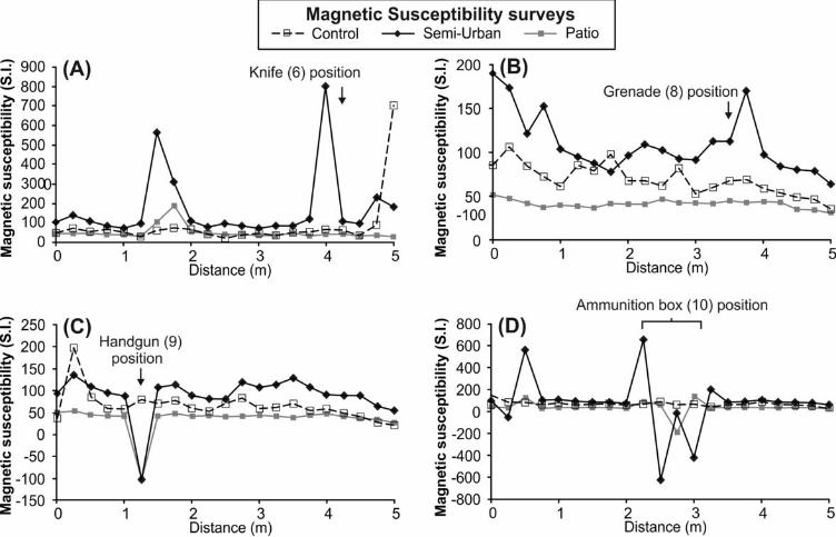
261
Magnetic susceptibility data for the post-burial, semi-urban environment also showed significant site 262
variations, with the same magnitude of high and low susceptibility readings as obtained in the control 263
dataset. In addition to the control isolated high anomalies again being present, several other isolated high 264
anomalies were present that could be correlated with 2 non-target object locations; (2) the bolt and (3) the 265
steel plate, and 4 target object locations; (4) the two breadknives, (5) the entrenching tool, (6) the single 266
breadknife, and (7) WWII hand grenade . Low isolated anomalies, with respect to background values, 267
could also be correlated with the remaining 4 target object locations; (9) the handgun, (10) the 268
ammunition box and (11) the spent mortar shell (Figs. 5 & 6). Magnetic susceptibility data for the post-269
burial patio environment had significantly less site variations, ranging from -242 to 496 S.I. units. In 270
addition to the control isolated high anomalies again being present, several other isolated high anomalies 271
were present that could be again correlated with 2 non-target object locations; (2) the bolt, (3) the steel 272
plate, and now 3 target object locations; (4) the two breadknives, (5) the entrenching tool and (7) the 273
WWII hand grenade (Figs. 5 & 6). Low isolated anomalies, with respect to background values, could 274
also be correlated with (9) the handgun, (10) the ammunition box and (11) the spent mortar shell locations 275
(Figs. 5 & 6). Selected 2D profiles are shown in Figure 6. Target detection rates with magnetic 276
susceptibility are therefore 100% (semi-urban) and 88% (patio) respectively. 277
278
Fluxgate gradiometry 279
280
Fluxgate gradiometry datasets (441 data points in each survey) for the control, post-burial semi-urban and 281
patio environment scenarios were very variable and geophysically ‘noisy’, having respective survey 282
median and 2σ values of -56.6 nT and 145 2σ (control), -3.1 nT and 157 2σ (semi-urban) and -45.8 nT 283
and 144 2σ (patio) surveys respectively. This would be expected in such heterogeneous ground 284
conditions, with a significant proportion of the datasets (32%, 31% and 30% respectively) not recording 285
data at sampling positions. However these non-sample areas were consistent which suggested the 286
instrument was not faulty nor calibrated incorrectly. With such a high proportion of the survey area not 287
recording values, the resulting gridded and contoured map view plots of the control, post-burial semi-288
urban and patio environment scenarios were not that useful, having significant large areas of high and low 289
magnetic gradiometry areas with respect to background values. However, 2D data profiles acquired over 290
the forensic objects did allow estimation of target detection to be undertaken, and some selected 2D 291
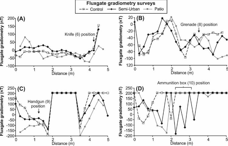
survey profiles are shown in Figure 7. 292
293
Within the post-burial semi-urban environment, high magnetic anomalies, with respect to background 294
values, could be correlated with 1 non-target object location; (3) the steel plate and 3 target object 295
locations; (4) two breadknives, (5) the entrenchment tool, (8) the WWI grenade and (10) the ammunition 296
box (Fig. 7). Within the post-burial domestic patio environment, high magnetic anomalies, with respect 297
to background values, could again be correlated with (3) the steel plate, and the same 4 target object 298
locations; (4) two breadknives, (6) the single breadknife, (8) the WWI hand grenade and (10) the 299
ammunition box (Fig. 7). 300
Fluxgate gradiometry survey results therefore gave a 50% (semi-urban) and 50% (patio) total target 301
detection success rate respectively. 302
303
Magnetic (potassium-vapour) gradiometry 304
305
Magnetic (potassium-vapour) gradiometry data for the three surveys (total data points of 5,437 (control), 306
3,729 (semi-urban) and 4,050 (patio) respectively) were also geophysically ‘noisy’. Respective survey 307
medians and 2σ of lower sensor total field data were 49,172.7 nT and 450 2σ (control), 49,182.4 nT and 308
1,112 2σ (semi-urban) and 49,184.5 nT and 1106 2σ (patio). Survey medians and 2σ of gradiometry data 309
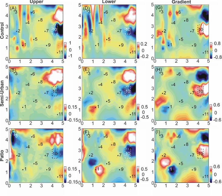
were 81.7 nT and 860 2σ (control), 88.5 nT and 742 2σ (semi-urban) and 94.8 nT and 708 2σ (patio) 310
indicating a generally good survey repeatability. Magnetic gradiometry map view plots of the control, 311
post-burial semi-urban and patio environment scenarios are shown in Figure 8, and detrended datasets 312
displayed in Figure 9 for comparison. It was found considerably easier to use the 2D profiles for 313
estimation of target detection (selected examples shown in Fig. 10) due to the high variability of 314
gradiometry measurements within the survey area, which made subtle anomalies difficult to identify in 315
plan-view plots (Fig. 8) even after detrending (Fig. 9). 316
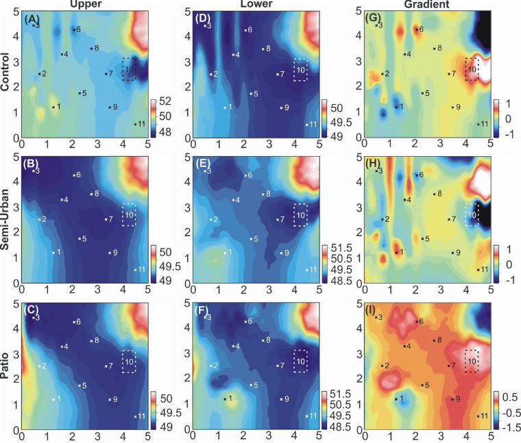
317
Within the post-burial semi-urban environment magnetic dataset, high magnetic anomalies, with respect 318
to background values, could be correlated with, of the non-target object locations; (3) the steel plate, and 319
of the target object locations; (6) the single breadknife, (7) the WWII hand grenade, (8) the WWI hand 320
grenade, (9) the handgun and (10) the ammunition box positions (Figs. 8, 9 & 10). Within the patio 321
scenario magnetic dataset, high magnetic anomalies, with respect to background values, could be 322
correlated with, of the non-target object locations; (2) the bolt and (3) the steel plate, and of the target 323
object locations; (4) the two breadknives, (6) the single breadknife, (7) the WWII hand grenade, (8) the 324
WWI hand grenade, (9) the handgun and (10) the ammunition box locations (Figs. 8, 9 & 10). Selected 325
2D survey profiles are shown in Figure 10. Potassium vapour gradiometry survey results therefore gave a 326
63% (semi-urban) and 75% (patio) total target detection success rate respectively. 327
328
Resistivity 329
330
Fixed-offset (0.5 m) resistivity data for the control dataset (441 data points) had resistance maximum / 331
minimum values of 111.7 Ω / 47.3 Ω with median of 75.0 Ω and 25.4 2σ value, therefore confirming that 332
the site was relatively electrically heterogeneous. The post-burial (semi-urban) 0.25 m and 0.50 m fixed-333
offset repeat surveys had resistance maximum / minimum values of 194.5 Ω / 76.0 Ω (25 cm) and 129.5 334
Ω / 51.5 Ω (50 cm), with median values of 121.6 Ω (25 cm) / 78.8 Ω (50 cm) and 37.2 2σ (25 cm) / 27.2 335
2σ (50cm) respectively. Data repeatability for the 0.5 m fixed-offset surveys was therefore generally 336
good, and can presumably be said for 0.25 m surveys despite the lack of a control dataset. 337
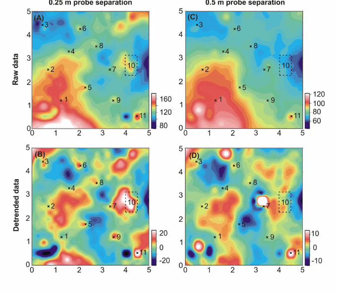
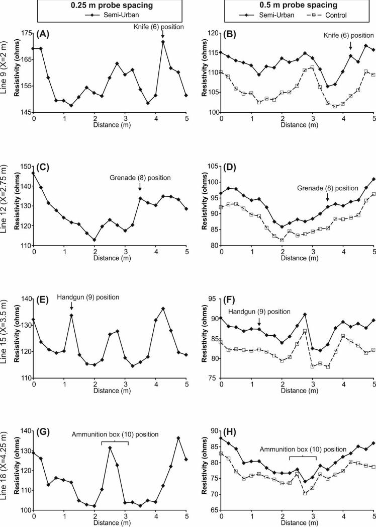
338
Within the post-burial semi-urban environment, high resistance anomalies in the 0.25 m fixed offset 339
survey, with respect to background values, could be correlated with target object locations of the (5) 340
entrenching tool, (6) the single knife, (7) the WWII hand grenade, (9) the handgun, (10) the ammunition 341
box and (11) the spent shell (Figs. 11 & 12). Low resistance anomalies, with respect to background 342
value, could be correlated with non-target object locations; (1) the brick and (3) the steel plate. 343
Within the semi-urban environment resistivity (0.5 m fixed-offset) survey, only high resistance 344
anomalies, with respect to background values, could be correlated with (10) the ammunition box and (11) 345
the spent shell locations (Figs. 11 & 12). Selected 2D profiles are shown in Figure 12. This therefore 346
gave a 63 % (25 cm) and 25 % (50 cm) total target detection success rate respectively. 347
348
Ground penetrating radar 349
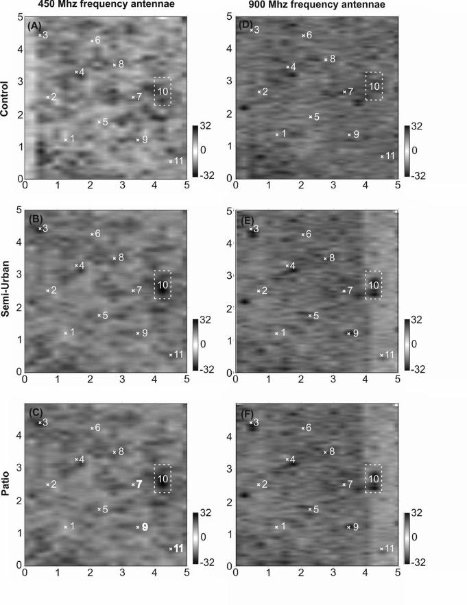
350
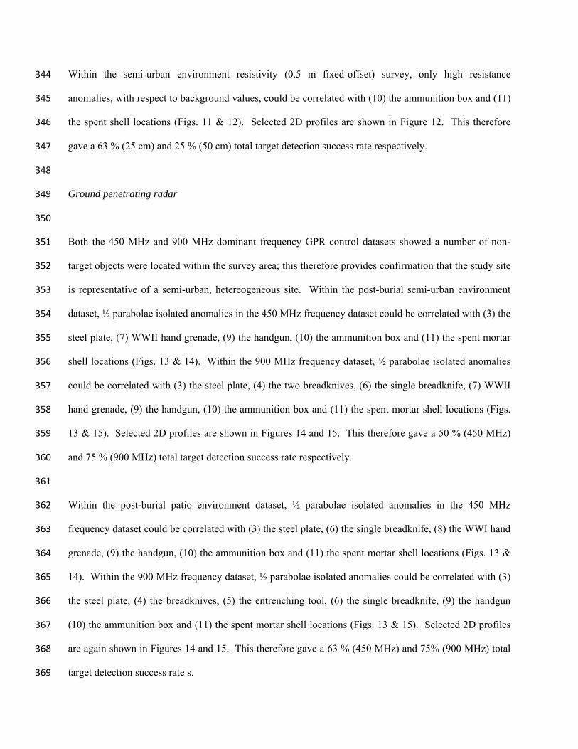
Both the 450 MHz and 900 MHz dominant frequency GPR control datasets showed a number of non-351
target objects were located within the survey area; this therefore provides confirmation that the study site 352
is representative of a semi-urban, hetereogeneous site. Within the post-burial semi-urban environment 353
dataset, ½ parabolae isolated anomalies in the 450 MHz frequency dataset could be correlated with (3) the 354
steel plate, (7) WWII hand grenade, (9) the handgun, (10) the ammunition box and (11) the spent mortar 355
shell locations (Figs. 13 & 14). Within the 900 MHz frequency dataset, ½ parabolae isolated anomalies 356
could be correlated with (3) the steel plate, (4) the two breadknives, (6) the single breadknife, (7) WWII 357
hand grenade, (9) the handgun, (10) the ammunition box and (11) the spent mortar shell locations (Figs. 358
13 & 15). Selected 2D profiles are shown in Figures 14 and 15. This therefore gave a 50 % (450 MHz) 359
and 75 % (900 MHz) total target detection success rate respectively. 360
361
Within the post-burial patio environment dataset, ½ parabolae isolated anomalies in the 450 MHz 362
frequency dataset could be correlated with (3) the steel plate, (6) the single breadknife, (8) the WWI hand 363
grenade, (9) the handgun, (10) the ammunition box and (11) the spent mortar shell locations (Figs. 13 & 364
14). Within the 900 MHz frequency dataset, ½ parabolae isolated anomalies could be correlated with (3) 365
the steel plate, (4) the breadknives, (5) the entrenching tool, (6) the single breadknife, (9) the handgun 366
(10) the ammunition box and (11) the spent mortar shell locations (Figs. 13 & 15). Selected 2D profiles 367
are again shown in Figures 14 and 15. This therefore gave a 63 % (450 MHz) and 75% (900 MHz) total 368
target detection success rate s. 369
Discussion 370
371
This section has been deliberately organised to answer and discuss the study objectives. 372
373
(1) Evaluate and find optimum magnetic detection technique(s) of the target buried material 374
375
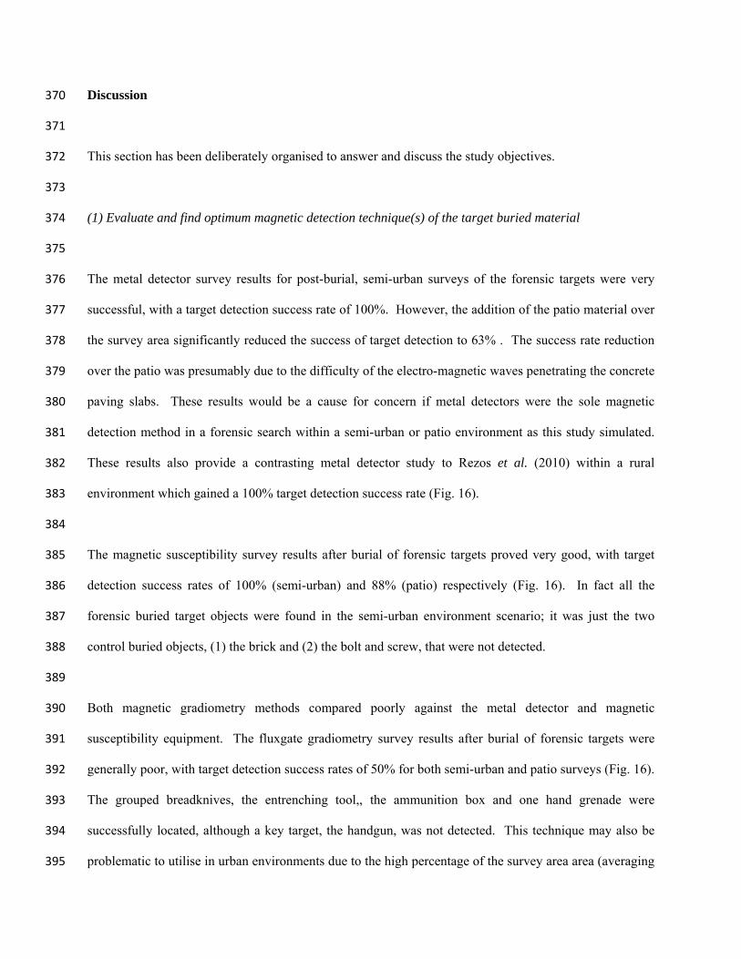
The metal detector survey results for post-burial, semi-urban surveys of the forensic targets were very 376
successful, with a target detection success rate of 100%. However, the addition of the patio material over 377
the survey area significantly reduced the success of target detection to 63% . The success rate reduction 378
over the patio was presumably due to the difficulty of the electro-magnetic waves penetrating the concrete 379
paving slabs. These results would be a cause for concern if metal detectors were the sole magnetic 380
detection method in a forensic search within a semi-urban or patio environment as this study simulated. 381
These results also provide a contrasting metal detector study to Rezos et al. (2010) within a rural 382
environment which gained a 100% target detection success rate (Fig. 16). 383
384
The magnetic susceptibility survey results after burial of forensic targets proved very good, with target 385
detection success rates of 100% (semi-urban) and 88% (patio) respectively (Fig. 16). In fact all the 386
forensic buried target objects were found in the semi-urban environment scenario; it was just the two 387
control buried objects, (1) the brick and (2) the bolt and screw, that were not detected. 388
389
Both magnetic gradiometry methods compared poorly against the metal detector and magnetic 390
susceptibility equipment. The fluxgate gradiometry survey results after burial of forensic targets were 391
generally poor, with target detection success rates of 50% for both semi-urban and patio surveys (Fig. 16). 392
The grouped breadknives, the entrenching tool,, the ammunition box and one hand grenade were 393
successfully located, although a key target, the handgun, was not detected. This technique may also be 394
problematic to utilise in urban environments due to the high percentage of the survey area area (averaging 395
31% over the three surveys) having out-of-range data recorded, as other authors have discussed 396
(Reynolds, 2011). 397
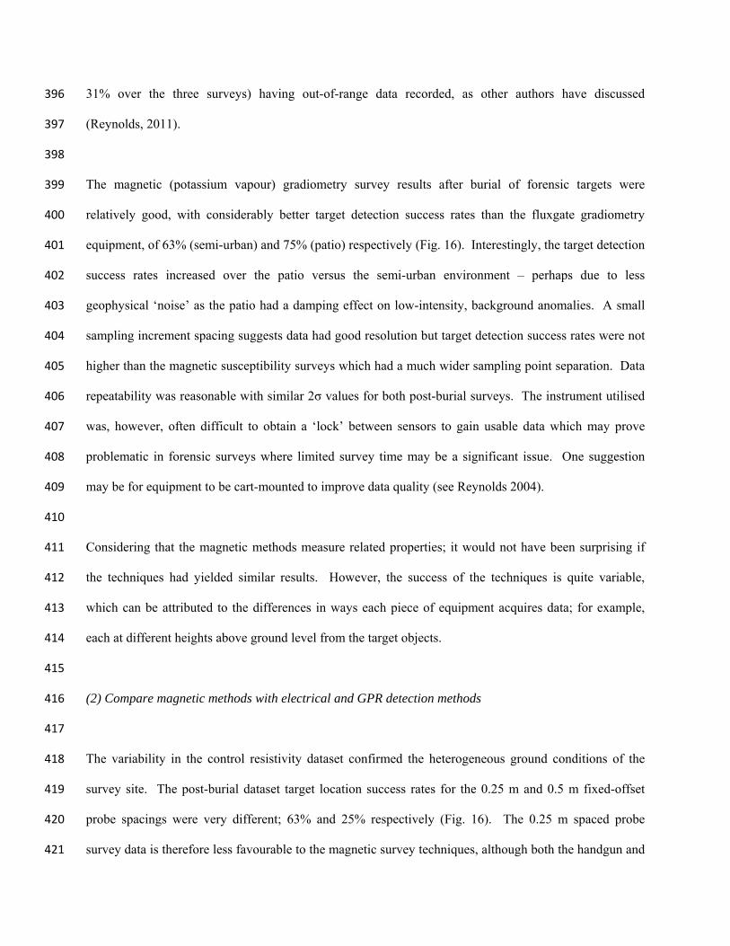
398
The magnetic (potassium vapour) gradiometry survey results after burial of forensic targets were 399
relatively good, with considerably better target detection success rates than the fluxgate gradiometry 400
equipment, of 63% (semi-urban) and 75% (patio) respectively (Fig. 16). Interestingly, the target detection 401
success rates increased over the patio versus the semi-urban environment – perhaps due to less 402
geophysical ‘noise’ as the patio had a damping effect on low-intensity, background anomalies. A small 403
sampling increment spacing suggests data had good resolution but target detection success rates were not 404
higher than the magnetic susceptibility surveys which had a much wider sampling point separation. Data 405
repeatability was reasonable with similar 2σ values for both post-burial surveys. The instrument utilised 406
was, however, often difficult to obtain a ‘lock’ between sensors to gain usable data which may prove 407
problematic in forensic surveys where limited survey time may be a significant issue. One suggestion 408
may be for equipment to be cart-mounted to improve data quality (see Reynolds 2004). 409
410
Considering that the magnetic methods measure related properties; it would not have been surprising if 411
the techniques had yielded similar results. However, the success of the techniques is quite variable, 412
which can be attributed to the differences in ways each piece of equipment acquires data; for example, 413
each at different heights above ground level from the target objects. 414
415
(2) Compare magnetic methods with electrical and GPR detection methods 416
417
The variability in the control resistivity dataset confirmed the heterogeneous ground conditions of the 418
survey site. The post-burial dataset target location success rates for the 0.25 m and 0.5 m fixed-offset 419
probe spacings were very different; 63% and 25% respectively (Fig. 16). The 0.25 m spaced probe 420
survey data is therefore less favourable to the magnetic survey techniques, although both the handgun and 421
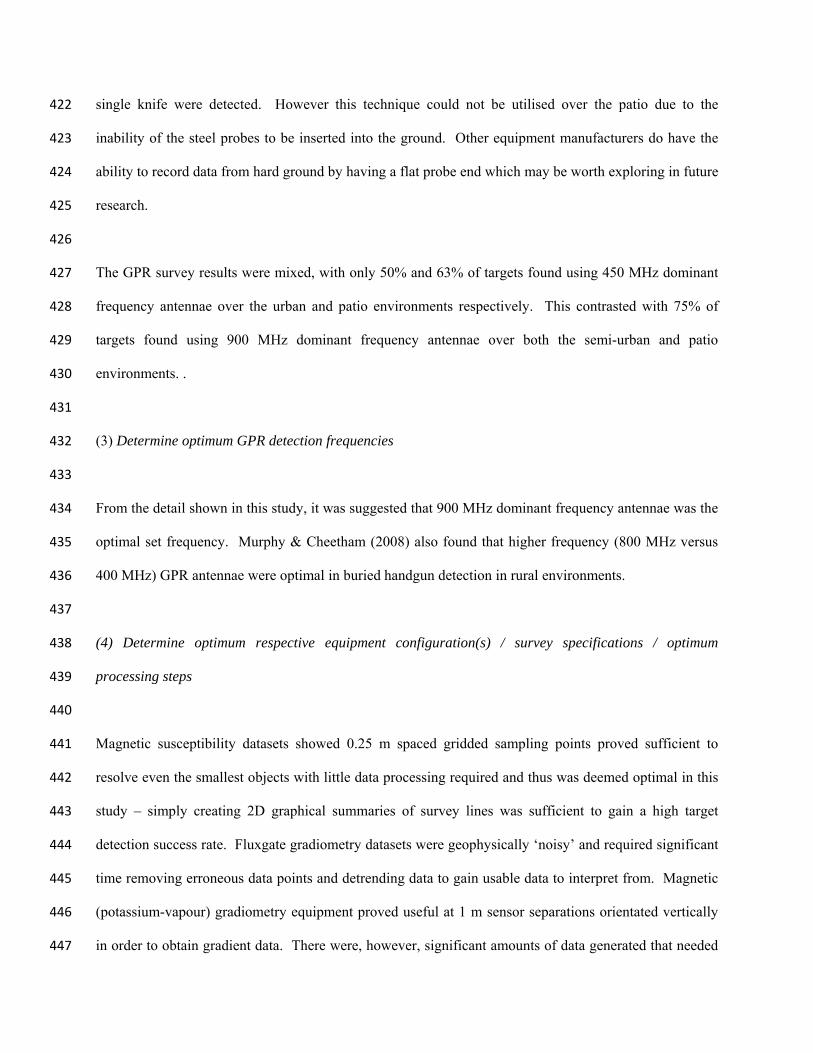
single knife were detected. However this technique could not be utilised over the patio due to the 422
inability of the steel probes to be inserted into the ground. Other equipment manufacturers do have the 423
ability to record data from hard ground by having a flat probe end which may be worth exploring in future 424
research. 425
426
The GPR survey results were mixed, with only 50% and 63% of targets found using 450 MHz dominant 427
frequency antennae over the urban and patio environments respectively. This contrasted with 75% of 428
targets found using 900 MHz dominant frequency antennae over both the semi-urban and patio 429
environments. . 430
431
(3) Determine optimum GPR detection frequencies 432
433
From the detail shown in this study, it was suggested that 900 MHz dominant frequency antennae was the 434
optimal set frequency. Murphy & Cheetham (2008) also found that higher frequency (800 MHz versus 435
400 MHz) GPR antennae were optimal in buried handgun detection in rural environments. 436
437
(4) Determine optimum respective equipment configuration(s) / survey specifications / optimum 438
processing steps 439
440
Magnetic susceptibility datasets showed 0.25 m spaced gridded sampling points proved sufficient to 441
resolve even the smallest objects with little data processing required and thus was deemed optimal in this 442
study – simply creating 2D graphical summaries of survey lines was sufficient to gain a high target 443
detection success rate. Fluxgate gradiometry datasets were geophysically ‘noisy’ and required significant 444
time removing erroneous data points and detrending data to gain usable data to interpret from. Magnetic 445
(potassium-vapour) gradiometry equipment proved useful at 1 m sensor separations orientated vertically 446
in order to obtain gradient data. There were, however, significant amounts of data generated that needed 447
to be processed and detrended before being usable. However, even after detrending of the datasets, 448
fluxgate gradiometry and magnetic (potassium vapour) gradiometry results were difficult to interpret in 449
plan-view plots due to the subtle anomalies caused by the target objects. In fact, it could be argued that 450
many of the target locations would not have been identifiable at all in these scenarios, had the control data 451
not been collected for comparison. Equipment operators also needed to be careful that a constant height 452
was maintained between the sensors and the ground surface to improve data quality which may be 453
problematic in forensic search scenarios on uneven ground. 454
455
The electrical resistivity 0.25 m fixed-offset probe spacing data was vastly superior to the 0.5 m offset 456
probe spaced datasets even when using the same sampling spacings; making the closer probe spacing the 457
more obvious one to utilise for such small and high resolution surveys. However, the amount of ground 458
covered in larger forensic search surveys using this configuration and 0.25 m grid sample spacings may 459
make this technique more problematic. 460
461
As mentioned, 900 MHz dominant frequency GPR antennae proved optimal, with a 0.025 m trace 462
sampling interval on 0.25 m spaced survey lines. Basic 2D profile data processing of gain filters and 463
background removal would prove sufficient for target detection although it would be deemed worthwhile 464
to generate horizontal ‘time-slices’ if targets were more subtle in comparison to heterogeneous ground, 465
and if processing time is allowed. 466
467
(5) Determine which technique(s) could determine target depth below ground level 468
469
Only GPR data could definitively determine depth of buried forensic target below ground level. Total 470
field magnetic data such as from the potassium vapour gradiometer and the bulk electrical resistivity data 471
could both be forward modelled to gain simple estimations of target depths if sufficient time and 472
specialist resources were available (see Juerges et al. 2010; Reynolds 2011 for examples). 473
474
(6) Determine if different metal types could be distinguished. 475
476
Distinguishing between different buried metallic object types was difficult using the equipment utilised; 477
Rezos et al. (2010), for example, used a higher specification metal detector which did allow some metal 478
differentiation to be determined. The resistivity survey results did differentiate between conductive (the 479
metal plate) and non-conductive (the brick) buried forensic targets which may be useful information for 480
forensic search investigators. 2D magnetic forward modelling of total field magnetic data would allow 481
the relative magnetic susceptibility contrast between the target object and the background material to be 482
assessed, (see, for example, Scott & Hunter 2004), but these would not be definitive values. 483
484
Finally it was determined that the metal detector, magnetic susceptibility meter, resistivity meter (if in 485
semi-urban environments) and a commercial GPR unit would be relatively easy for forensic search 486
investigators to acquire, process and interpret for buried forensic targets. Metal detector equipment is 487
relatively cheap but also arguably the simplest to use and to generate data from that forensic search teams 488
could interpret buried target locations. When considering both the semi-urban and patio scenarios, 489
however, the magnetic susceptibility equipment provided the best target detection rates, with relatively 490
few additional non-target anomalies. The equipment was also relatively cheap and easy to process into a 491
visual data-plot. The magnetic susceptibility dataset from the patio scenario showed very low variability 492
at points other than at target and non-target object locations, so would be optimal in this environment 493
considering the low number of false positives. GPR data could be viewed in real-time and suspected 494
burial positions marked during the field work. Resistivity data would need to be downloaded and line 495
profiles generated in any data graphical packages of which there are many. The fluxgate gradiometer and 496
magnetic (potassium-vapour) gradiometer are only recommended to be utilised by experienced operators 497
due to the difficulty of calibration, operation and data processing. 498
499
It should, however, be noted that the success rates from these surveys are alone not enough to determine 500
optimum techniques and equipment configurations for detection of buried metallic objects. One must 501
also consider that a technique which is capable of detecting all target objects may also be overly sensitive 502
to background anomalies. For example, the metal detector, though capable of detecting all 8 target 503
objects, also detected an additional 6 background anomalies. This means that only 57% of the anomalies 504
can be attributed to buried targets. 505
506
Conclusions 507
508
From the results of this study, usable geophysical techniques gaining the highest buried forensic object 509
target success rates in semi-urban environments were (in descending order); magnetic susceptibility, 510
metal detection, 900 MHz GPR and electrical resistivity (0.25 m fixed-offset probes), magnetic 511
(potassium vapour) gradiometry, 450 MHz GPR, fluxgate gradiometry and electrical resistivity (0.5 m 512
fixed-offset probes) (Fig. 16). Usable geophysical techniques gaining the highest buried forensic object 513
target success rates in patio environments (in descending order) were; magnetic susceptibility, magnetic 514
(potassium vapour) gradiometry, 900 MHz GPR, metal detection, 450 MHz GPR, and fluxgate 515
gradiometry (Fig. 16). Note resistivity surveys were not utilised in the patio environment. It was worth 516
noting that the magnetic susceptibility had a considerably higher success rate than the other magnetic 517
equipment utilised, i.e. compared to the metal detector and the gradiometers, despite them measuring 518
similar properties and the potassium vapour gradiometer having a closer sample point spacing. 519
520
Concerns were raised in this study over the use of metal detectors and GPR detection equipment solely 521
for detection of buried forensic targets, as important objects such as knives and hand grenades were not 522
detected by even the higher frequency GPR configuration, particularly beneath the patio. It is therefore 523
recommended that the easy to utilise and high target success rates of the magnetic susceptibility 524
equipment should be used as a complementary tool for forensic search investigators in the search for 525
buried objects such as those used in this study. The bulk electrical resistivity technique also showed 526
potential due to its relatively quick collection time and reasonably high detection rate. Unlike GPR data 527
processing, resistivity data processing is relatively straightforward (given available software and operator 528
experience) and can produce either 2D profiles or a single mapview image which can then be interpreted. 529
530
Acknowledgements 531
532
Keele University are thanked for land donation for the test site. Laura Ore, Sarah Reid, Leanne Patrick 533
and Emily Postlethwaite are thanked for field assistance. Michael Hannah is thanked for replica handgun 534
donation. Geophysical equipment has been funded by a 2003 SRIF2 equipment bid. 535
536
537
References 538
539
ACHEROY, M. 2007. Mine action: status of sensor technology for close-in and remote detection of anti-540
personnel mines. Near Surface Geophysics, 5, 43-56. 541
542
BILLINGER, M. S. 2009. Utilizing ground penetrating radar for the location of a potential human burial 543
under concrete. Canadian Society of Forensic Science Journal, 42, 200-209. 544
545
BAVUSI, M., RIZZO, E. & LAPENNA, V. 2006. Electromagnetic methods to characterize the Savoia di 546
Lucania waste dump in southern Italy. Environmental Geology, 51, 301-308. 547
548
CONGRAM, D. R. 2008. A clandestine burial in Costa Rica: prospection and excavation. Journal of 549
Forensic Sciences, 53, 793-796. 550
551
CURRAN, A. M., PRADA, P. A. & FURTON, K. G. 2010. Canine human scent identifications with post-552
blast debris collected from improvised explosive devices. Forensic Science International, 199, 103-108. 553
554
DAVENPORT, G. C. 2001. Remote sensing applications in forensic investigations. Historical 555
Archaeology, 35, 87–100. 556
557
DIONNE, C. A., SCHULTZ, J. J., MURDOCK II R. A & SMITH, S. A. 2011. Detecting buried metallic 558
weapons in a controlled setting using a conductivity meter. Forensic Science International, 208, 18-24. 559
560
DUPRAS, T. L., SCHULTZ, J. J., WHEELER, S. M. & WILLIAMS, L. J. 2006. Forensic Recovery of 561
Human Remains: Archaeological Approaches. Taylor & Francis, 232 pp. 562
563
FENNING, P. J. & DONNELLY, L. J. 2004. Geophysical techniques for forensic investigations. In: Pye, 564
K., Croft, D.J. (eds), Forensic Geoscience: Principles, Techniques and Applications. Geological Society, 565
London, Special Publications, 232, 11-20. 566
567
HARRISON, M. & DONNELLY, L. J. 2009. Locating concealed homicide victims: developing the role 568
of geoforensics. In: Ritz, K., Dawson, L., Miller, D. (eds), Criminal and Environmental Soil Forensics, 569
Springer Publishing, pp. 197-219. 570
571
HUNTER, J. & COX, M. 2005. Forensic archaeology: advances in theory and practice. Routledge 572
Publishers, 256 pp. 573
574
JERVIS, J. R., PRINGLE, J. K. & TUCKWELL, G. W. 2009. Time-lapse resistivity surveys over 575
simulated clandestine graves. Forensic Science International, 192, 7-13. 576
577
JOL, H. M. 2009. Ground penetrating radar: theory and applications. Elsevier Publications, Amsterdam, 578
The Netherlands, 524 pp. 579
580
JUERGES, A., PRINGLE, J. K., JERVIS, J. R. & MASTERS, P. 2010. Comparisons of magnetic surveys 581
over simulated clandestine graves in contrasting burial environments. Near Surface Geophysics, 8, 529-582
539. 583
584
LINFORD, N. 2004. Magnetic ghosts: Mineral magnetic measurements on Roman and Anglo-Saxon 585
graves. Archaeological Prospection, 11, 167–180. 586
587
MARCHETTI, M., CAFARELLA, L., DI MAURO, D. & ZIRIZZOTI, A. 2002. Ground magnetometric 588
surveys and integrated geophysical methods for solid buried waste detection: a case study. Annals of 589
Geophysics, 45, 563-573. 590
591
MILLER, P. S. 1996. Disturbance in the soil: finding buried bodies and other evidence using ground 592
penetrating radar. Journal of Forensic Sciences, 41, 648-652. 593
594
MILSOM, J. & ERIKSEN, A. 2011. Field Geophysics. 4th Edition. John Wiley & Sons, 232 pp. 595
596
MURPHY, J. & CHEETHAM, P. 2008. A comparative study into the effectiveness of geophysical 597
techniques for the location of buried handguns. Abstract for a presentation at the Geoscientific 598
Equipment & Techniques at Crime Scenes, Forensic Geoscience Group Conference, Geological Society 599
of London, Burlington House, London, 17th December. 600
601
NOBES, D. C. 2000. The search for ‘‘Yvonne’’: a case example of the delineation of a grave using near-602
surface geophysical methods. Journal of Forensic Sciences, 45, 715–721. 603
604
PARKER, R., RUFFELL, A., HUGHES, D. & PRINGLE, J. 2010. Geophysics and the search of 605
freshwater bodies: a review. Science & Justice, 50, 141-149. 606
607
PRINGLE, J. K., RUFFELL, A., JERVIS, J. R. MCKINLEY, J., DONNELLY, L., PIRRIE, D., 608
MORGAN, R., JARVIS, K. & HARRISON, M. 2012a. The use of earth science methods in terrestrial 609
forensic searches. Earth Science Reviews, 114(1-2), 108-123. 610
611
PRINGLE, J. K., JERVIS, J. R., HANSEN, J. D., CASSIDY, N. J., JONES, G. M., CASSELLA, J. P. 612
2012b. Geophysical monitoring of simulated clandestine graves using electrical and Ground Penetrating 613
Radar methods: 0-3 years. Journal of Forensic Sciences, 57(6), 1467-1486. 614
615
PRINGLE, J. K. & JERVIS, J. R. 2010. Electrical resistivity survey to search for a recent clandestine 616
burial of a homicide victim, UK. Forensic Science International, 202(1-3), e1-e7. 617
618
PRINGLE, J. K., JERVIS, J., CASSELLA, J. P. & CASSIDY, N. J. 2008. Time-lapse geophysical 619
investigations over a simulated urban clandestine grave. Journal of Forensic Sciences, 53, 1405-1417. 620
621
REBMANN, A., DAVID, E. & SORG, M. H. 2000. Cadaver dog handbook: forensic training and tactics 622
for the recovery of human remains. CRC Press, Florida, USA, 232 pp. 623
624
REYNOLDS, J. M. 2011. Applied and environmental geophysics. 2nd edition, John Wiley & Sons, 625
Chichester, UK, 636 pp. 626
627
REYNOLDS, J.M. 2004. Environmental geophysics investigations in urban areas. First Break, 22, 63-69. 628
629
REZOS, M. M., SCHULTZ, J. J., MURDOCK II R.A. & SMITH, S.A. 2010. Controlled research 630
utilizing a basic all-metal detector in the search for buried firearms and miscellaneous weapons. Forensic 631
Science International, 195, 121-127. 632
633
RUFFELL, A. & KULESSA, B. 2009. Application of geophysical techniques in identifying illegally 634
buried toxic waste. Environmental Forensics, 10, 196–207. 635
636
SCHULTZ, J. J. 2008. Sequential monitoring of burials containing small pig cadavers using ground-637
penetrating radar. Journal of Forensic Sciences, 53, 279–287. 638
639
SCHULTZ, J. J., COLLINS, M. E. & FALSETTI, A. B. 2006. Sequential monitoring of burials 640
containing large pig cadavers using ground-penetrating radar. Journal of Forensic Sciences, 51, 607–616. 641
642
SCOTT, J. & HUNTER, J.R. 2004. Environmental influences on resistivity mapping for the location of 643
clandestine graves. In: PYE, K. & CROFT, D.J. (eds) 2004. Forensic Geoscience: Principles, Techniques 644
and Applications. Geological Society, London, Special Publications, 232, 33-38. 645
646
TOMS, C., ROGERS, C. B. & SATHYAVAGISWARAN, L. 2008. Investigations of homicides interred 647
in concrete – The Los Angeles experience. Journal of Forensic Sciences, 53, 203-207. 648
649
WESSEL, P. & SMITH, W. H. F. 1998. New improved version of Generic Mapping Tools. EOS 650
Transactions, 55, 293-305. 651
652
FIGURE CAPTIONS 653
654
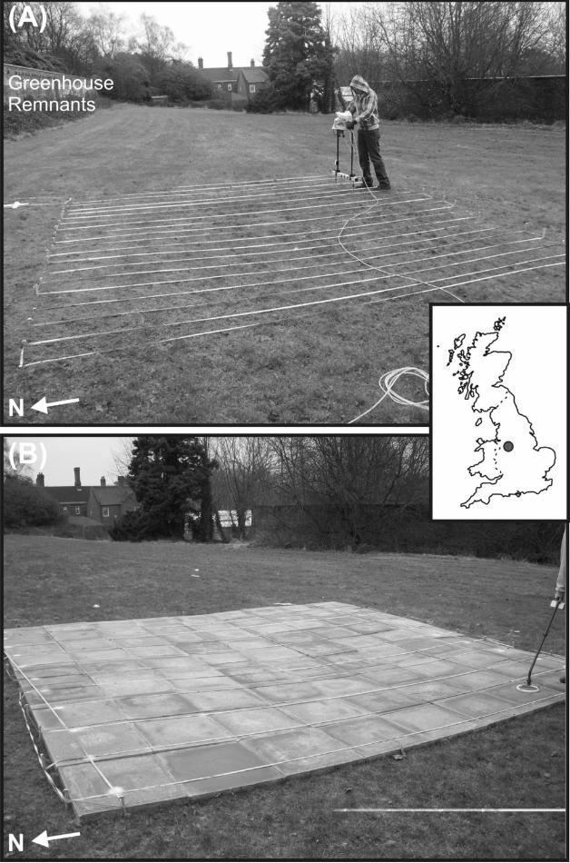
Fig. 1. Photographs of the 5 m by 5 m forensic test site on campus showing (a) semi-urban environment 655
and (b) simulated domestic concrete patio scenario on the same area with location map (inset). Survey 656
tapes on survey lines are shown. 0,0 position for all surveys is SW corner. 657
658
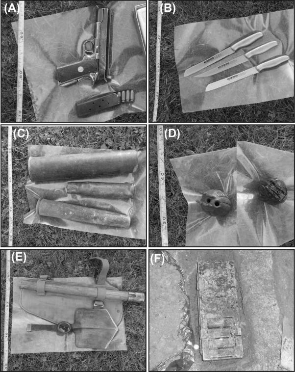
Fig. 2. Selected photographs of forensic buried test objects. (A) Colt Government Cup Replica .45 659
calibre automatic handgun with solid brass ammunition; (B) Three domestic stainless steel kitchen bread 660
knives; (C) 1943 75 mm M18 shell and two WWII smaller diameter spent shells; (D) (left) WWII allied 661
hand grenade and (right) WWI allied Mk.1 No.5 decommissioned hand grenade; (E) 1943 allied wooden-662
handled entrenchment tool and; (F) UK mortar ammunition box (containing 2 shell casings shown in C). 663
See Table 2 for details. 664
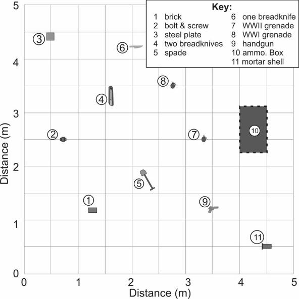
665
Fig. 3. Sitemap showing location of buried forensic objects (see key for details) for both semi-urban 666
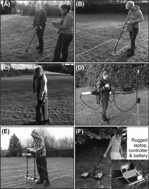
environment and patio scenarios (Fig. 2 for selected object photographs). 667
668
Fig. 4. Photographs of geophysical equipment used in this study. (A) Bloodhound Tracker™ IV metal 669
detector; (B) Bartington™ magnetic susceptibility probe MS.1 with 0.3 m diameter probe; (C) Geoscan™ 670
FM-15 fluxgate gradiometer; (D) GSMP-40™ potassium vapour magnetic gradiometer with sensors 1 m 671
vertically separated; (E) Geoscan™ RM15-D mobile probe resistivity meter and; (F) pulseEKKO™ 1000 672
Ground Penetrating Radar equipment showing 450 MHz dominant frequency, bistatic fixed-offset 673
antennae. 674
675
Fig. 5. Magnetic susceptibility selected 2D profiles for control, semi-urban and patio surveys with 676
respective target positions marked. (A) Profile 9 (X=2 m) over target (6) single knife; (B) profile 12 677
(X=2.75 m) over target (8) WWI hand grenade; (C) profile 15 (X=3.5 m) over target (9) handgun and; 678
(D) profile 18 (X=4.25 m) over target (10) ammunition box (all marked). See key for survey type and 679
Table 1 for details. 680
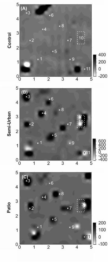
681
Fig. 6. Magnetic susceptibility processed, gridded and contoured map view data plots of (A) pre-burial 682
control with interpreted isolated anomalies, with respect to background values, marked (see text); (B) 683
post-burial semi-urban environment and; (C) post-burial patio garden environment respectively. Scale for 684
(A) and (B) are the same. S.I. (dimensionless) units are used (see text). See Table 2 for target 685
descriptions. 686
687
Fig. 7. Fluxgate gradiometry selected 2D surveys profiles for control, semi-urban and patio surveys with 688
respective target positions marked. (A) Profile 9 (X=2 m) over target (6) single knife; (B) profile 12 689
(X=2.75 m) over target (8) WWI hand grenade; (C) profile 15 (X=3.5 m) over target (9) handgun and; 690
(D) profile 18 (X=4.25 m) over target (10) ammunition box (all marked). See key for survey type and 691
Table 1 for details. 692
693
Fig. 8. Magnetic (potassium vapour) gradiometry processed, gridded and contoured map-view plots using 694
upper sensor, lower sensor and gradient for pre-burial, post-burial semi-urban and patio environments (A-695
I, respectively) Units in 1000nT. See Table 2 for target descriptions. 696
697
Fig. 9. Magnetic (potassium vapour) gradiometry processed, detrended, gridded and contoured map view 698
plots using upper sensor, lower sensor and gradient for pre-burial, post-burial semi-urban and pre-burial 699
patio environments (A-I, respectively). Units in 1000nT. See Table 2 for target descriptions. 700
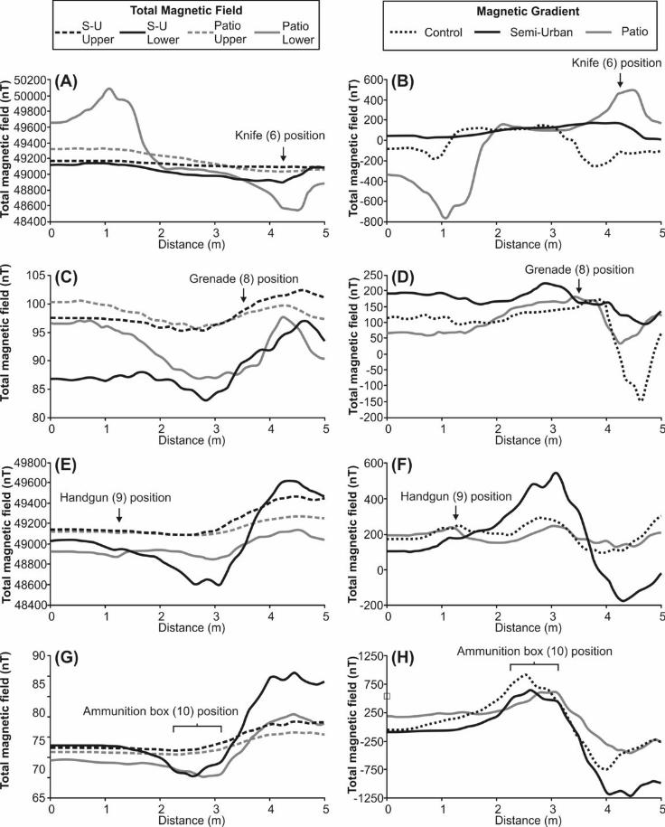
701
Fig. 10. Magnetic (potassium vapour) gradiometry with total magnetic (left) and gradient (right) selected 702
2D survey profiles for control, semi-urban and patio surveys with respective target positions marked. 703
(A/B) Profile 9 (X=2 m) over target (6) single knife; (C/D) profile 12 (X=2.75 m) over target (8) WWI 704
hand grenade; (E/F) profile 15 (X=3.5 m) over target (9) handgun and; (G/H) profile 18 (X=4.25 m) over 705
target (10) ammunition box (all marked). See key for sensors, survey type and Table 1 for details. 706
707
Fig. 11. Post-burial, semi-urban, bulk ground-resistivity contour plots using raw and detrended datasets 708
with 0.25 (A and B respectively) m and 0.5 m (C and D respectively) probe spacings. Note the relatively 709
high anomalies corresponding to the knife (6), handgun (9) and mortar shell (11). See Table 2 for target 710
descriptions. 711
712
Fig. 12. Bulk-ground resistivity 2D profiles for selected targets using 0.25 m and 0.5 m probe separations 713
with units in Ohms (Ω). Note generally high resistivity anomalies associated with targets with the 714
exception of 0.5 m probe separation survey over the ammunition box (H). 715
716
Fig. 13. GPR time-slices over the test site using 450 MHZ (A-C) and 900 MHz (D-F) dominant frequency 717
antennae with units in relative amplitudes. Some relatively high and relatively low amplitude anomalies 718
correspond to target positions. See Table 2 for target descriptions. 719
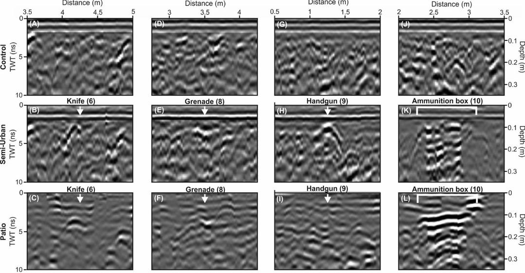
720
Fig. 14. 450 MHz GPR processed selected 2D profiles. (A-C) Profile 9 (X=2 m) over target (6) single 721
knife; (D-F) profile 12 (X=2.75 m) over target (8) WWI hand grenade; (G-I) profile 15 (X=3.5 m) over 722
target (9) handgun and; (J-L) profile 18 (X=4.25 m) over target (10) ammunition box for control, semi-723
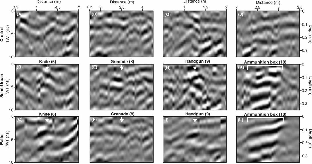
urban and patio environment scenarios respectively (all marked). See Table 1 for details. 724
725
Fig. 15. 900 MHz GPR processed selected 2D profiles. (A-C) Profile 9 (X=2 m) over target (6) single 726
knife; (D-F) profile 12 (X=2.75 m) over target (8) WWI hand grenade; (G-I) profile 15 (X=3.5 m) over 727
target (9) handgun and; (J-L) profile 18 (X=4.25 m) over target (10) ammunition box for control, semi-728
urban and patio environment scenarios respectively (all marked). See Table 1 for details. 729
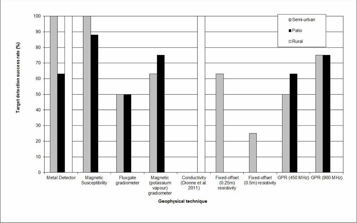
730

Fig. 16. Summary graph showing percentage total of target detection success rates for the different 731
geophysical techniques trialled in semi-urban, patio and rural environments (see key). Note rural 732
environment results are from Rezos et al. (2010) and Dionne et al. (2010) for metal detector and 733
conductivity surveys respectively. 734
735
TABLE CAPTIONS 736
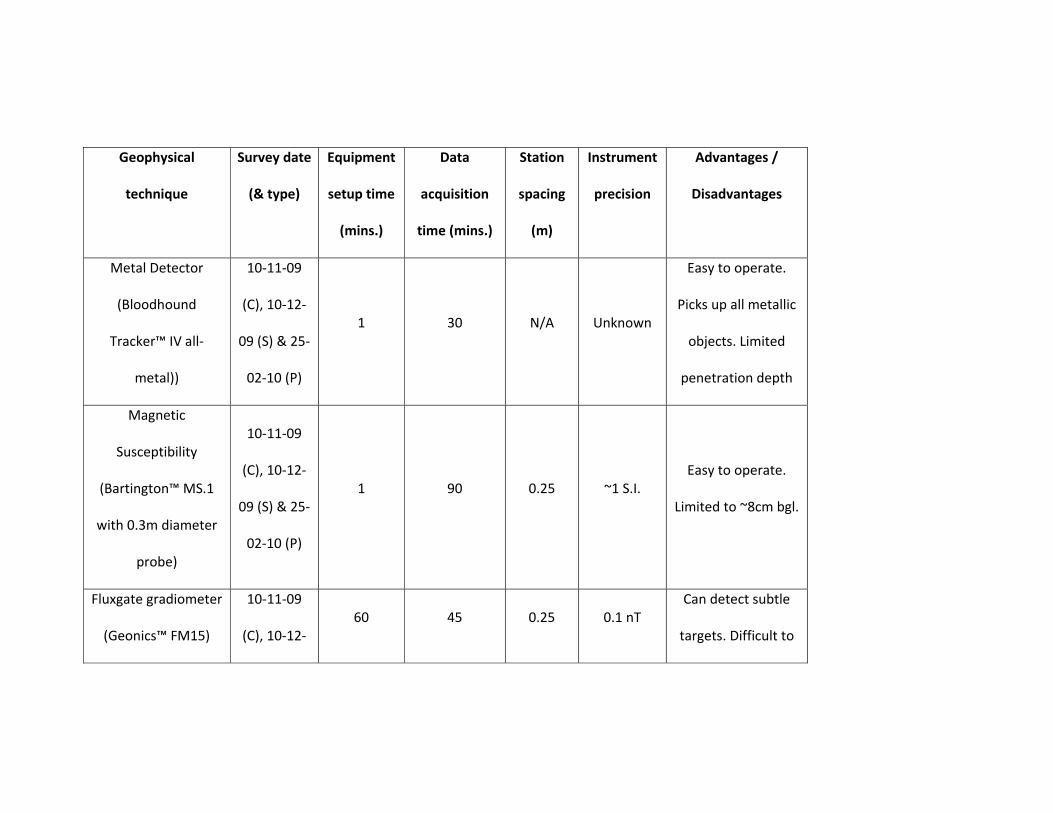
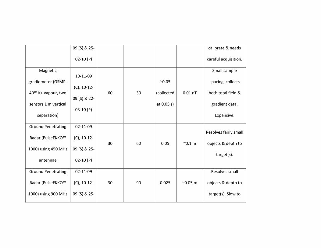
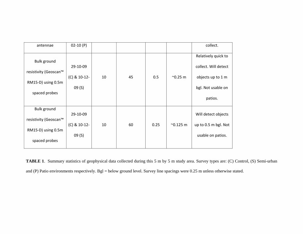
737
TABLE 1. Summary statistics of geophysical data collected during this 5 m by 5 m study area. 738
Survey types are: (C) Control, (S) Semi-urban and (P) Patio environments respectively. Bgl = 739
below ground level. Survey line spacings were 0.25 m unless otherwise stated. 740
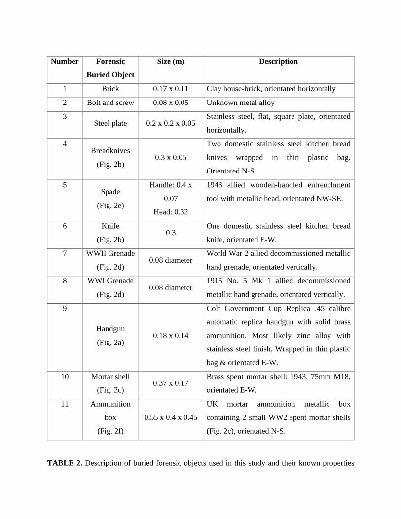
741 TABLE 2. Description of buried forensic objects used in this study and their known properties 742
(captions show photographs in Fig. 2). Object numbers refer to those shown in Fig. 3 and in 743
geophysical datasets. 744
745
Geophysical
technique
Survey date
(& type)
Equipment
setup time
(mins.)
Data
acquisition
time (mins.)
Station
spacing
(m)
Instrument
precision
Advantages /
Disadvantages
Metal Detector
(Bloodhound
Tracker™ IV all-
metal))
10-11-09
(C), 10-12-
09 (S) & 25-
02-10 (P)
1 30 N/A Unknown
Easy to operate.
Picks up all metallic
objects. Limited
penetration depth
Magnetic
Susceptibility
(Bartington™ MS.1
with 0.3m diameter
probe)
10-11-09
(C), 10-12-
09 (S) & 25-
02-10 (P)
1 90 0.25 ~1 S.I. Easy to operate.
Limited to ~8cm bgl.
Fluxgate gradiometer
(Geonics™ FM15)
10-11-09
(C), 10-12-60 45 0.25 0.1 nT
Can detect subtle
targets. Difficult to
09 (S) & 25-
02-10 (P)
calibrate & needs
careful acquisition.
Magnetic
gradiometer (GSMP-
40™ K+ vapour, two
sensors 1 m vertical
separation)
10-11-09
(C), 10-12-
09 (S) & 22-
03-10 (P)
60 30
~0.05
(collected
at 0.05 s)
0.01 nT
Small sample
spacing, collects
both total field &
gradient data.
Expensive.
Ground Penetrating
Radar (PulseEKKO™
1000) using 450 MHz
antennae
02-11-09
(C), 10-12-
09 (S) & 25-
02-10 (P)
30 60 0.05 ~0.1 m
Resolves fairly small
objects & depth to
target(s).
Ground Penetrating
Radar (PulseEKKO™
1000) using 900 MHz
02-11-09
(C), 10-12-
09 (S) & 25-
30 90 0.025 ~0.05 m
Resolves small
objects & depth to
target(s). Slow to
antennae 02-10 (P) collect.
Bulk ground
resistivity (Geoscan™
RM15-D) using 0.5m
spaced probes
29-10-09
(C) & 10-12-
09 (S)
10 45 0.5 ~0.25 m
Relatively quick to
collect. Will detect
objects up to 1 m
bgl. Not usable on
patios.
Bulk ground
resistivity (Geoscan™
RM15-D) using 0.5m
spaced probes
29-10-09
(C) & 10-12-
09 (S)
10 60 0.25 ~0.125 m
Will detect objects
up to 0.5 m bgl. Not
usable on patios.
TABLE 1. Summary statistics of geophysical data collected during this 5 m by 5 m study area. Survey types are: (C) Control, (S) Semi-urban
and (P) Patio environments respectively. Bgl = below ground level. Survey line spacings were 0.25 m unless otherwise stated.
Number Forensic
Buried Object
Size (m) Description
1 Brick 0.17 x 0.11 Clay house-brick, orientated horizontally
2 Bolt and screw 0.08 x 0.05 Unknown metal alloy
3 Steel plate 0.2 x 0.2 x 0.05
Stainless steel, flat, square plate, orientated
horizontally.
4 Breadknives
(Fig. 2b) 0.3 x 0.05
Two domestic stainless steel kitchen bread
knives wrapped in thin plastic bag.
Orientated N-S.
5 Spade
(Fig. 2e)
Handle: 0.4 x
0.07
Head: 0.32
1943 allied wooden-handled entrenchment
tool with metallic head, orientated NW-SE.
6 Knife
(Fig. 2b) 0.3
One domestic stainless steel kitchen bread
knife, orientated E-W.
7 WWII Grenade
(Fig. 2d) 0.08 diameter
World War 2 allied decommissioned metallic
hand grenade, orientated vertically.
8 WWI Grenade
(Fig. 2d) 0.08 diameter
1915 No. 5 Mk 1 allied decommissioned
metallic hand grenade, orientated vertically.
9
Handgun
(Fig. 2a) 0.18 x 0.14
Colt Government Cup Replica .45 calibre
automatic replica handgun with solid brass
ammunition. Most likely zinc alloy with
stainless steel finish. Wrapped in thin plastic
bag & orientated E-W.
10 Mortar shell
(Fig. 2c) 0.37 x 0.17
Brass spent mortar shell: 1943, 75mm M18,
orientated E-W.
11 Ammunition
box
(Fig. 2f)
0.55 x 0.4 x 0.45
UK mortar ammunition metallic box
containing 2 small WW2 spent mortar shells
(Fig. 2c), orientated N-S.
TABLE 2. Description of buried forensic objects used in this study and their known properties

(captions show photographs in Fig. 2). Object numbers refer to those shown in Fig. 3 and in
geophysical datasets.