1

Chapter 6: Study Designs

Experimental vs. Quasi-experimental (Experimental consist of random assignment to treatment and control conditions)

Two conflicting forces:

1. Sufficient rigor and specificity to make firm conclusions

2. Limitations of money, time, cooperation, and protection of human subjects limits the design options.

2

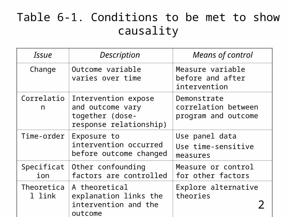
Table 6-1. Conditions to be met to show causality

Issue Description Means of control

Change Outcome variable varies over time

Measure variable before and after intervention

Correlation Intervention expose and outcome vary together (dose-response relationship)

Demonstrate correlation between program and outcome

Time-order Exposure to intervention occurred before outcome changed

Use panel data

Use time-sensitive measures

Specification Other confounding factors are controlled

Measure or control for other factors

Theoretical link A theoretical explanation links the intervention and the outcome

Explore alternative theories

3

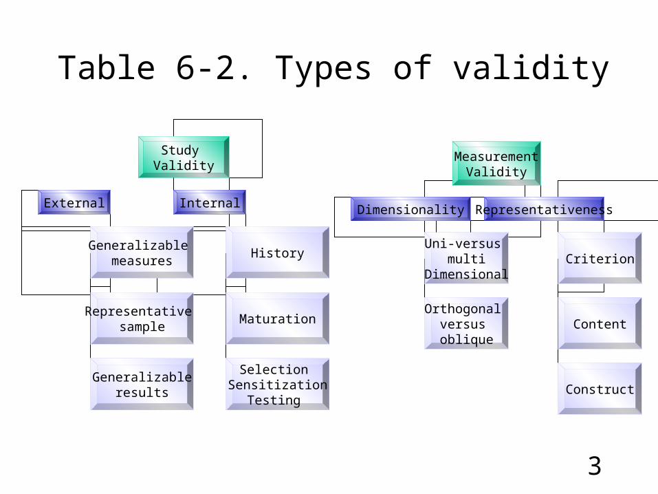
Table 6-2. Types of validity

Study Validity

External Internal

Generalizable measures

Representative sample

Generalizableresults

History

Maturation

Selection Sensitization

Testing

MeasurementValidity

Dimensionality Representativeness

Uni-versus multi

Dimensional

Orthogonal versus oblique

Criterion

Content

Construct

4

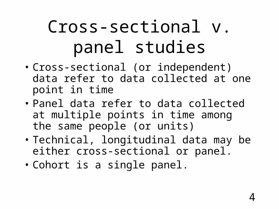
Cross-sectional v. panel studies

• Cross-sectional (or independent) data refer to data collected at one point in time

• Panel data refer to data collected at multiple points in time among the same people (or units)

• Technical, longitudinal data may be either cross-sectional or panel.

• Cohort is a single panel.

5

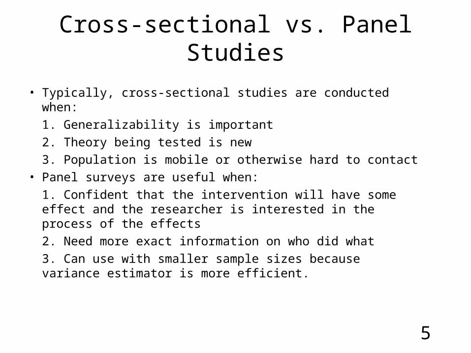
Cross-sectional vs. Panel Studies

• Typically, cross-sectional studies are conducted when:

1. Generalizability is important

2. Theory being tested is new

3. Population is mobile or otherwise hard to contact

• Panel surveys are useful when:

1. Confident that the intervention will have some effect and the researcher is interested in the process of the effects

2. Need more exact information on who did what

3. Can use with smaller sample sizes because variance estimator is more efficient.

6

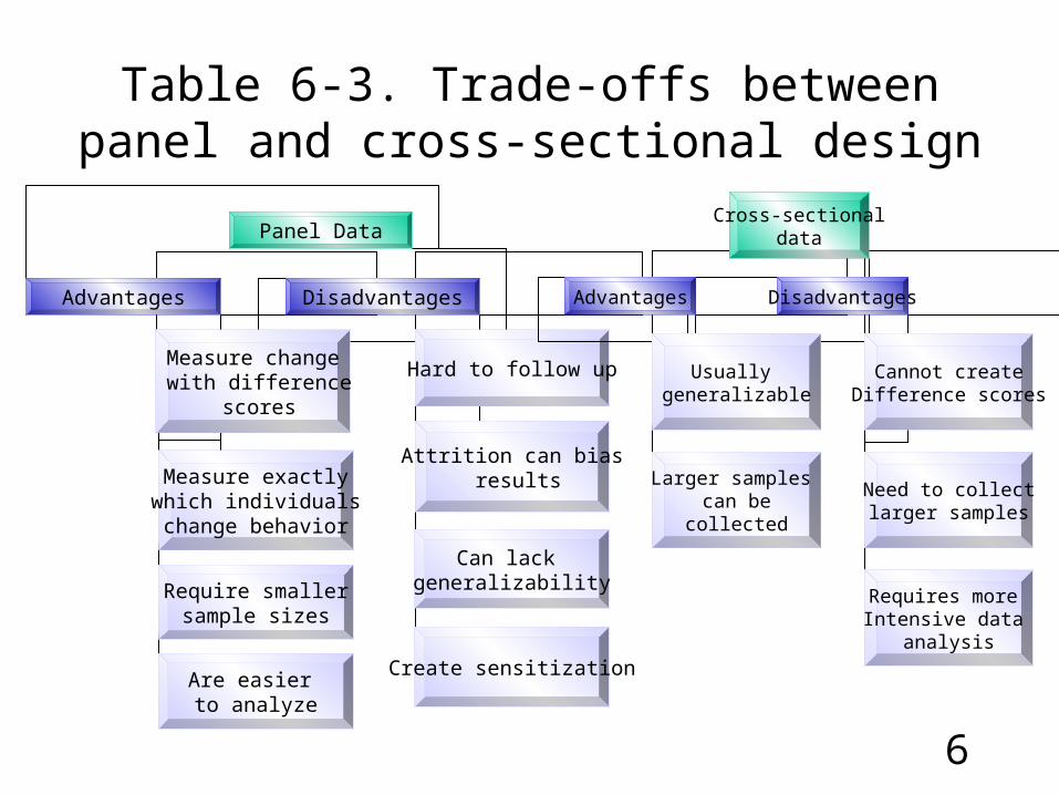
Table 6-3. Trade-offs between panel and cross-sectional design

Panel Data

Advantages Disadvantages

Measure change with difference

scores

Measure exactly which individuals change behavior

Require smallersample sizes

Hard to follow up

Attrition can bias results

Can lack generalizability

Are easier to analyze

Create sensitization

Cross-sectionaldata

Advantages Disadvantages

Usually generalizable

Larger samples can be

collected

Cannot createDifference scores

Need to collectlarger samples

Requires more Intensive data

analysis

7

4 Types of Validity

• Study validity

• Measurement validity

• Statistical validity

• Program validity

8

External vs. Internal Validity

External:

Generalizability of research results

Internal:

Conclusions made are accurate

9

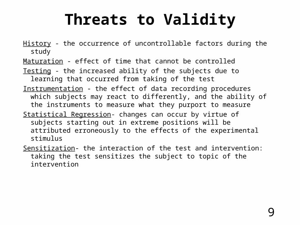
Threats to Validity

History - the occurrence of uncontrollable factors during the study

Maturation - effect of time that cannot be controlled

Testing - the increased ability of the subjects due to learning that occurred from taking of the test

Instrumentation - the effect of data recording procedures which subjects may react to differently, and the ability of the instruments to measure what they purport to measure

Statistical Regression- changes can occur by virtue of subjects starting out in extreme positions will be attributed erroneously to the effects of the experimental stimulus

Sensitization- the interaction of the test and intervention: taking the test sensitizes the subject to topic of the intervention

10

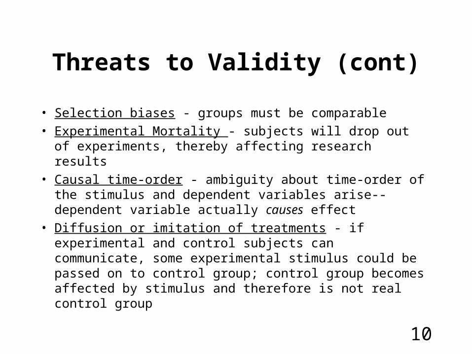
Threats to Validity (cont)

• Selection biases - groups must be comparable• Experimental Mortality - subjects will drop out of

experiments, thereby affecting research results• Causal time-order - ambiguity about time-order of the

stimulus and dependent variables arise--dependent variable actually causes effect

• Diffusion or imitation of treatments - if experimental and control subjects can communicate, some experimental stimulus could be passed on to control group; control group becomes affected by stimulus and therefore is not real control group

11

Threats to Validity (cont)

• Compensation - experimental group receiving something considered valuable, therefore control group might be given compensation, thereby no longer true control group

• Compensatory rivalry - control subjects, deprived of stimulus,might work harder to compensate

• Demoralization - feelings of deprivation might cause control group to give up

12

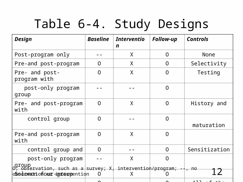
Table 6-4. Study DesignsDesign Baseline Intervention Follow-up Controls

Post-program only -- X O None

Pre-and post-program O X O Selectivity

Pre- and post- program with O X O Testing

post-only program group -- -- O

Pre- and post-program with O X O History and

control group O -- O maturation

Pre-and post-program with O X O

control group and O -- O Sensitization

post-only program group -- X O

Solomon four-group O X O

O -- O All of the above

-- X O

-- -- O

O, observation, such as a survey; X, intervention/program; --, no observation or intervention

13

Table 6-5. Hypothetical Study Outcome Scores (panel study)

Received

Pretest Program Posttest Differences Effect of

Group 1 1000 Yes 1400 + 400 Program, pretest, time

Group 2 1000 1200 + 200 Pretest and time

Group 3 Yes 1100 + 100 Program and time

Group 4 1050 + 50 Time

14

Description of Observation Groups

Obs. Time Other Obs. Intervention?

1 Pre-test With Post-test Yes

2 Post-test With Pre-test Yes

3 Pre-test With Post-test No

4 Post-test With Pre-test No

5 Post-test No Pre-test Yes

6 Post-test No Pre-test No

15

Program and Validity Threat Estimates for the Hypothetical Panel Study

Factors Amount Factors Calculation

Program, Pre-test, & Time +400 Sensitization=150 400-250

Pre-test & Time +200 Pre-test=150 200-50

Program & Time +100 Program=50 100-50

Time + 50 Time = 50

16

Selecting a Study Design

1. Ethical issues - Study design should not contain any unethical procedures.

2. Real-world considerations (Practical and administrative issues)

3. Technical issues -

1. Random assignment to conditions

2. Finding comparison groups

3. Time series design

4. Collect baseline information

5. Multivariate techniques

6. Threats to validity

17

Good Research Designs:

1. Are ethical - provide best quality of services

2. Provide the most reliable and valid data

3. Measures whatever happens in the field

4. Avoids making false conclusions

18

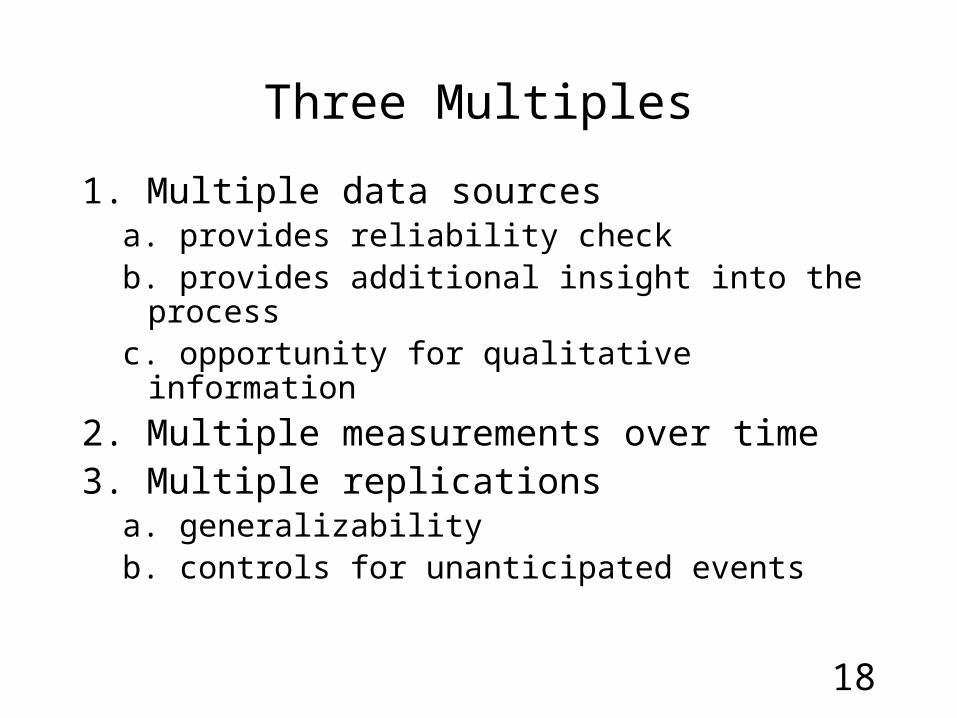
Three Multiples

1. Multiple data sourcesa. provides reliability checkb. provides additional insight into the processc. opportunity for qualitative information

2. Multiple measurements over time3. Multiple replications

a. generalizabilityb. controls for unanticipated events

19

Chapter 7: Sampling & sample size

• Sampling: What type of sample to select

• Sample size & power: How many units are needed

AND

• If I have N units, is that sufficient?

• Sample type and size will dramatically influence study costs and procedures.

20

Probability Sampling

1. Simple random sampling - EPSEM

2. Systematic

3. Stratified & Cluster

4. Census

5. Multistage

6. Probability proportional to size (PPS)

21

Non-Probability Sampling

1. Convenience

2. Purposive - planned selection of specific cases.a. Quota sampling - numbers of elements that fit

certain criteria are included in the sample.

b. Key informants - Non-probability, purposive selection of respondents who fit certain conditions.

22

Sample Size Determination

1. Resources

2. Plan of analysis - the sample must be large enough to:a. Produce uni- and bivariate crosstabs.

b. Provide for accurate estimates of proportions.

23

Four Methods for Sample Size Calculation

1. Tabulation

2. Proportions

3. Differences

4. Power

24

1. Tabulation Method

• At least 50 cases for each category of key independent variables

• At least 5 cases in any cell of a cross tabulation

• Not often used because in practice distributions are unknown

25

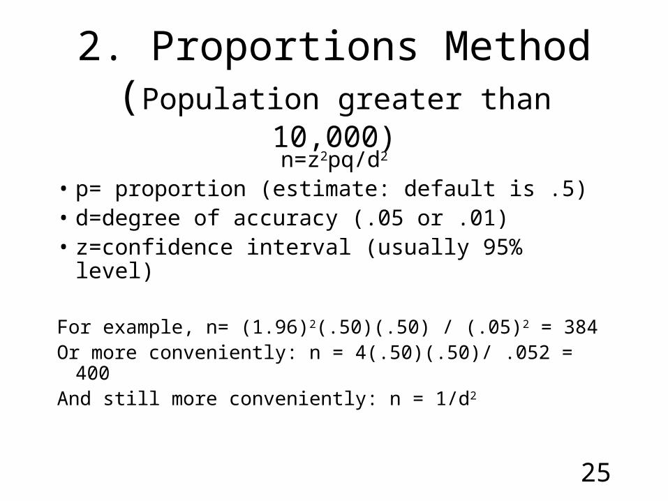
2. Proportions Method(Population greater than 10,000)

n=z2pq/d2

• p= proportion (estimate: default is .5)• d=degree of accuracy (.05 or .01)• z=confidence interval (usually 95% level)

For example, n= (1.96)2(.50)(.50) / (.05)2 = 384Or more conveniently: n = 4(.50)(.50)/ .052 = 400And still more conveniently: n = 1/d2

Figure 7-1: Schematic of Multistage Sample Selection.

Counties (Cluster)

Blocks (Cluster)

Households(Primary SamplingUnit)

A

B

27

Correction Factors

• Design effect - correction for clustering of sample. Some communities have more variation than others so you compute the ratio of variances to get design effect parameter

• Sampling significant fraction of the population. If it exceeds 5% then use correction n/(1+n/N)

28

3. Differences between Proportions

• Minimum difference you wish to be significant

• n’ = 2z2pq/(d’)2

For example, assume .4 proportion and expect that a .1 difference is sig.

n’ = 2(1.96)2(.40)(.60)/(.10)2 = 184Thus you would need 200 subjects in the

control and 200 in the treatment group

29

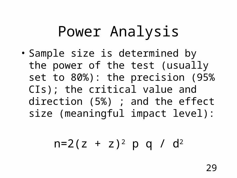
Power Analysis

• Sample size is determined by the power of the test (usually set to 80%): the precision (95% CIs); the critical value and direction (5%) ; and the effect size (meaningful impact level):

n=2(z + z)2 p q / d2

30

Power

• Critical value, Alpha, Type 1

• Sample size

• Effect size

• Power, Beta, Type 2 error

31

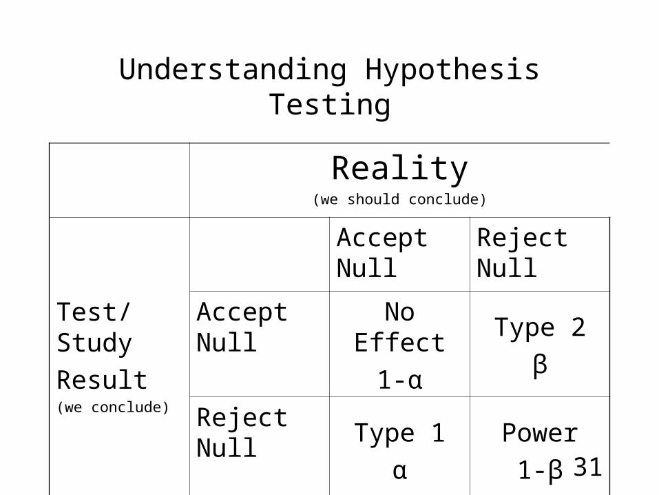
Understanding Hypothesis Testing

Reality(we should conclude)

Test/Study

Result(we conclude)

Accept Null Reject Null

Accept Null No Effect

1-α

Type 2

β

Reject Null Type 1

α

Power

1-β

32

Chapter 8: Data Collection

Survey Question Design - Simplicity

1. Simple language - Use simple terms and sentence structure

2. Short questions

3. Avoid double-barreled questions

4. Use common concepts

5. Present manageable tasks - Don’t expect the respondent to keep in mind numerous categories.

6. Shared definitions - For example, when you use the term family what does it mean. Include all definitions and instructions in questionnaires.

7. Questionnaire construction easy-> specific -> demos

33

Rules for Recall

1. Bounded

2. Reference period (six months or less)

3. “Average” - In a typical day, how many hours do you spend watching TV?

4. Landmarks

5. Provide Cues

34

Experimental Evidence

1. Specificity - specific questions are more accurate

2. Close-ended questions

3. Offer a “no opinion” or “neutral” option

4. Include a middle category, but don’t read it

5. Measure intensity whenever possible

6. Be sensitive to question order

funnel from general to specific

7. Wording effects are real and powerful

8. Ask multiple questions on a topic

35

Tools at Hand

1. Circulate drafts of your questionnaire

2. Use FGDs and interviews w/ target audience

3. Borrow freely from standard ?-naires (Standard questionnaires must still be pre-tested since (a) language constantly changes, and (b) questions affected by neighboring questions)

4. Conduct declared and undeclared pretests

36

Pre-test, pre-test, pre-test!!

1. Variation: you want a 30/70 variation not a 5/95

2. Meaning: How does the respondent interpret the question. (Ask them: “What does this mean to you?”)

3. Task difficulty - Make questions simple

4. Interest & Attention: Vary the question responses and phrasing

37

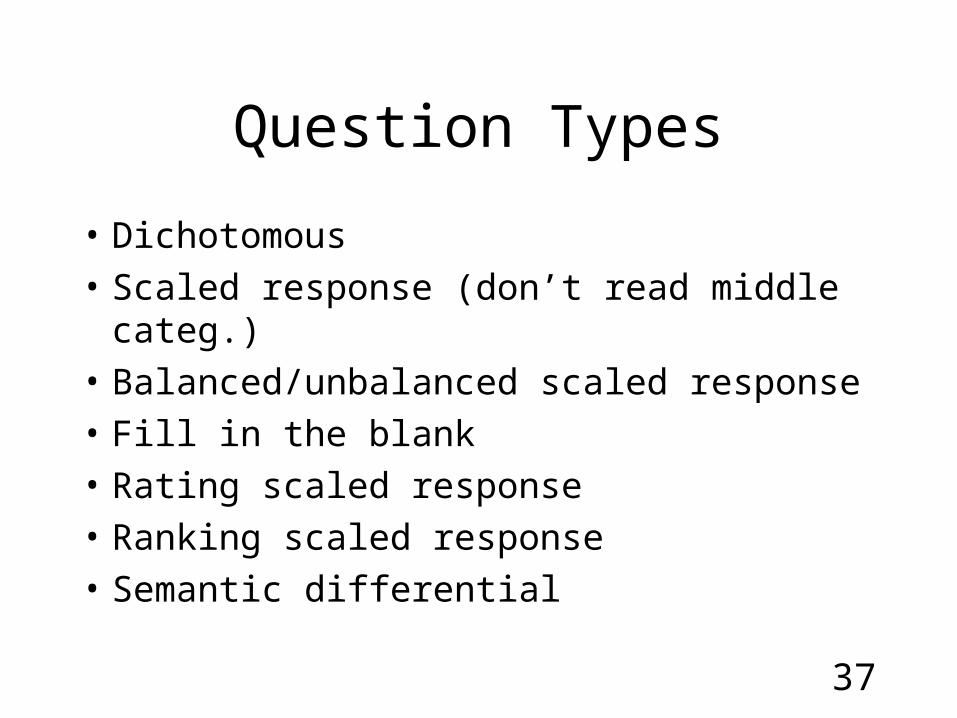
Question Types

• Dichotomous

• Scaled response (don’t read middle categ.)

• Balanced/unbalanced scaled response

• Fill in the blank

• Rating scaled response

• Ranking scaled response

• Semantic differential

38

Box 8-1: Question Examples

Dichotomous (binary choice)In the past 6 months, have you seen any commercial on TV related to illegal

substance abuse?0. No 1. Yes

SCALED RESPONSE, BALANCED (LIKERT)How much did you like that TV commercial that you saw regarding substance

abuse? Did you like it very much, somewhat like it, somewhat dislike it, or dislike it very much?

• Very much liked it 2. Somewhat dislike it3. Somewhat liked it 4. Very much disliked itSCALED RESPONSE, UNBALANCEDIn the past 6 months, how often have you seen commercials on TV related to

illegal substance abuse?1. Never 2. Sometimes 3. Often 4. All the time

39

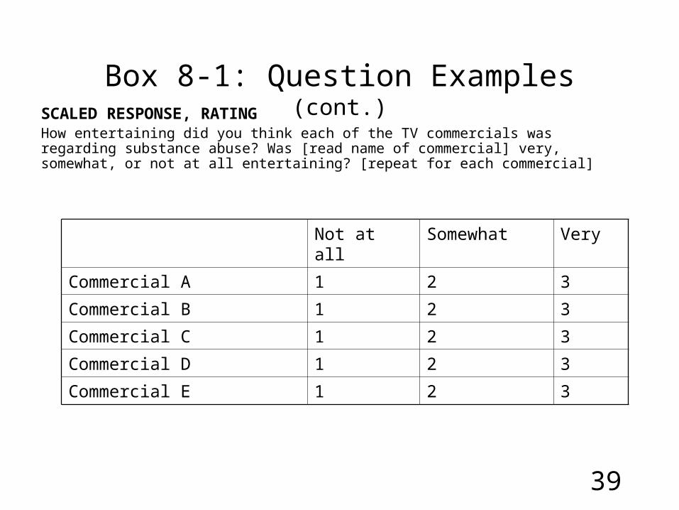
Box 8-1: Question Examples (cont.)SCALED RESPONSE, RATINGHow entertaining did you think each of the TV commercials was regarding substance abuse? Was [read name of commercial] very, somewhat, or not at all entertaining? [repeat for each commercial]

Not at all Somewhat Very

Commercial A 1 2 3

Commercial B 1 2 3

Commercial C 1 2 3

Commercial D 1 2 3

Commercial E 1 2 3

40

SCALED RESPONSE, RANKINGPlease rank the six TV commercials on substance abuse according to how entertaining each was. Which commercial was most entertaining? What second most? Third most? Fourth? Fifth? Least entertaining? [place the rank order next to each commercial.]

Commercial A ____

Commercial B ____

Commercial C ____

Commercial D ____

Commercial E ____

Commercial F ____

Box 8-1: Question Examples (cont.)

41

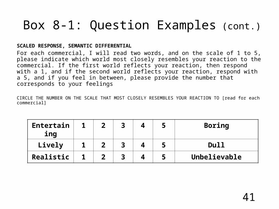
SCALED RESPONSE, SEMANTIC DIFFERENTIAL

For each commercial, I will read two words, and on the scale of 1 to 5, please indicate which world most closely resembles your reaction to the commercial. If the first world reflects your reaction, then respond with a 1, and if the second world reflects your reaction, respond with a 5, and if you feel in between, please provide the number that corresponds to your feelings

CIRCLE THE NUMBER ON THE SCALE THAT MOST CLOSELY RESEMBLES YOUR REACTION TO [read for each commercial]

Entertaining 1 2 3 4 5 Boring

Lively 1 2 3 4 5 Dull

Realistic 1 2 3 4 5 Unbelievable

Box 8-1: Question Examples (cont.)

42

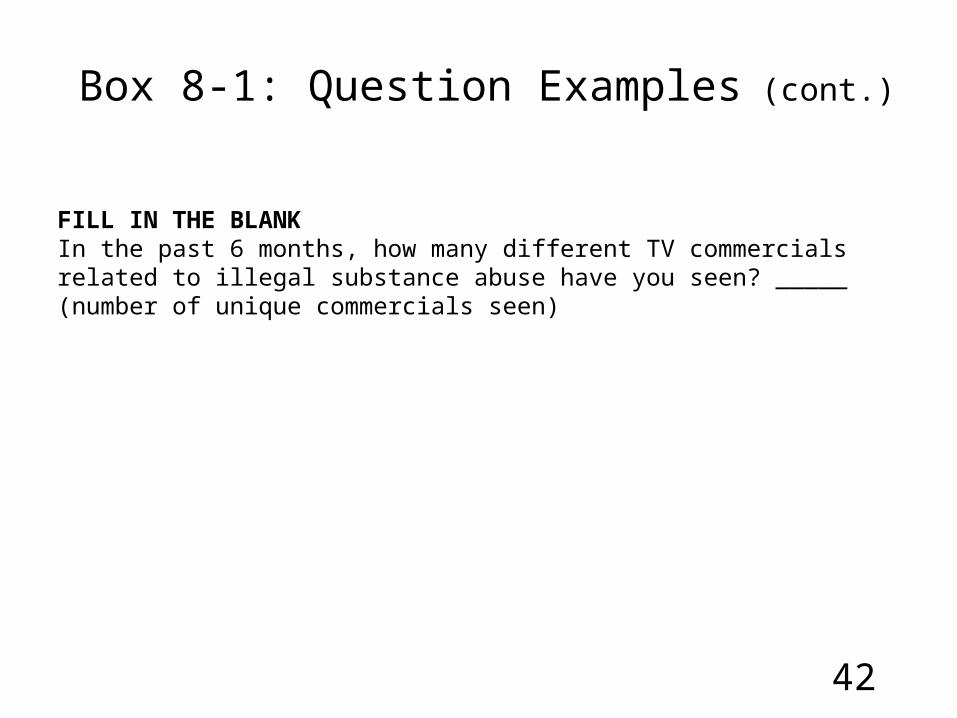
FILL IN THE BLANKIn the past 6 months, how many different TV commercials related to illegal substance abuse have you seen? _____ (number of unique commercials seen)

Box 8-1: Question Examples (cont.)

43

Pre-testing the Questionnaire

1. Flow: Does the survey flow

2. Question order: Do a question logically come after another

3. Skip patterns: Keep to a minimum and make sure you don’t lose anyone

4. Length: At least less than one hour, probably shorter (Phone < face-to-face) (Volunteer < Paid) (Commercial < Pro-social)

44

Questionnaire Development

1. Close-ended questions (double cost) probe meaning in open-ended follow-ups

2. Length should be less than twice final length

3. Respondents should resemble target population

4. Pretest 25-75

45

Survey Types

Three main types:

• Phone (30-50%) --> 70-90%

• Mail (30-50%) --> 70-90%

• In-person

Degree of interaction

Cost

Which is best for what

46

CATI/CASI

• CATI advantageous in that skip patterns are responses are built in

• Interviewer doesn’t need to handle paper

• CASI adds flexibility and anonymity

• CASI can include graphics and audiovisual aids; data are entered directly into the database reducing errors

47

Response RatesAffected by: 1) relevance of study2) reputation of surveyor3) quality of the survey4) persistence of researchers5) incentives ($1/$5 in envelop)6) first class postage7) pre-notification and cover lettersEstimates• Mail general population HH: (30-50%) --> 70-90%• Mail professional lists: (40-60%) --> 70-90%• Phone Surveys: (40-60%) --> 70-90%• In-person: 70%

48

TDM

• Specified importance of pre-notification letters, follow-up postcards, follow-up surveys, follow-up phone calls

• Importance of mailing package and attractiveness of survey, incentives

• Improved RRs dramatically make data more accurate

49

Data Management

1. Dataset Formats - Spreadsheets, Database Programs, Statistical Programs, Editors

2. DBMSCOPY – used to copy datasets from one program to another

50

Dataset Terminology

Usually:

1. Cases=observations=records=respondents=rows

2. Variables=questions=columns (usually)

3. Variables have labels; values have labels; and values should be stored as numeric if they are numbers and strings if characters.

51

Logical Operators

• & - and• | - or• = - equals• == - is equal to• != - not equal to (also ~)

52

Labeling variables & their values

label variable - describes the variable

--> label variable income “level of income”

label define - defines a value label

--> label define yesno 0"no” 1"yes”

label value - attaches a label to a variable

--> label value espabs yesno

--> label value espcal yesno

53

Miscellaneous Important Topics

• Saving Files

• Batch Files (Also known as "do files“ or “program files”)

• Line Delimiters # delim ; label define education 1 “primary” 2

“secondary” 3 “college” 4 “post-col”;

54

Variable Creation

Generate new variables to:

• Collapse or recode old variables

• Combine variables into new ones

• Scale creation

55

Baseline Survey

AppendDatasets

Cross-sectional SampleFollow up Survey

Panel SampleFollow up Survey

MergeDatasets

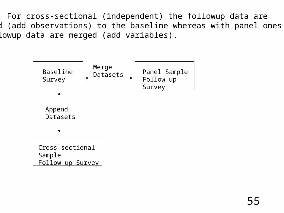
Box 8-4: For cross-sectional (independent) the followup data are appended (add observations) to the baseline whereas with panel ones, the followup data are merged (add variables).

56

Chapter 9: Univariate Analysis & Scale Creation

Univariate Analysis

1. To understand data

2. To determine whether normally distributed

3. To interpret results

57

Univariate (cont.)

• Central tendency – mean, median, & mode

• Variance – IQV, range, & standard deviation

• Skewness – symmetry around the mean

• Kurtosis – “peakiness” platykurtic & leptokurtic

Figure 9-1 Normal distributions with increasing variances

0.00

0.10

0.20

0.30

0.40

-10.

00

-9.1

0

-8.2

0

-7.3

0

-6.4

0

-5.5

0

-4.6

0

-3.7

0

-2.8

0

-1.9

0

-1.0

0

-0.1

0

0.80

1.70

2.60

3.50

4.40

5.30

6.20

7.10

8.00

8.90

9.80

Standardized Score (Z)

SD=1

SD=2

SD=5

59

Scales

• Index – count or sum of dichotomous items

• Scale – combination of multiple items can be summed or otherwise combined

• Scale construction = factor analysis

60

Scale Construction

1. Creation

a. Scale - sum of attitude items (agree/disagree)

b. Index - count of items (true/false; items known)

2. Intepretation & labeling - Scales are described and labeled (factor analysis used to determine dimensionality)

3. Reliability - Cronbach’s alpha (ranges of .70 - .85)

61

Table 9.1 Factor Loading for FP Attitudes in Bolivia

. factor q16a_q16k, mineigen(1)(obs=776) (principal factors; 1 factor retained) Factor Eigenvalue Difference Proportion Cumulative________________________________________________________ 1 1.99474 1.42690 0.9499 0.9499 2 0.56783 0.32492 0.2704 1.2203 3 0.24292 0.12418 0.1157 1.3360 4 0.11874 0.01287 0.0565 1.3925 5 0.10587 0.09228 0.0504 1.4430 6 0.01359 0.13177 0.0065 1.4494 7 _0.11818 0.02549 _0.0563 1.3931 8 _0.14368 0.03767 _0.0684 1.3247 9 _0.18134 0.05027 _0.0864 1.2384 10 _0.23161 0.03734 _0.1103 1.1281 11 _0.26895 . _0.1281 1.0000

62

Table 9.1 (cont.)

Factor Loadings Variable | 1 Uniqueness__________+_____________________ q16a | 0.33430 0.88825 q16b | 0.49446 0.75551 q16c | 0.37567 0.85887 q16d | 0.48924 0.76065 q16e | 0.56024 0.68613 q16f | 0.56732 0.67814 q16g | 0.40823 0.83335 q16h | 0.33692 0.88648 q16i | 0.45267 0.79509 q16j | 0.35864 0.87137 q16k | 0.09260 0.99142 

63

Table 9-2. Factor Loading Results for Baltimore TV Viewership

I am going to read a list of types of television shows; please tell me which if any you watch on a regular basis. [Pause after each for yes or no]

[ ] 1 Informational/Documentary (i.e., Discovery Channel, Learning Channel, PBS)

[ ] 2 News Programs (i.e., Nightly News, 60 Minutes)

[ ] 3 Cable News Channels (i.e., CNN, CNBC)

[ ] 4 Daytime Dramas (i.e., One Life to Live)

[ ] 5 Sitcoms (i.e., Seinfeld, Friends)

[ ] 6 Dramas (i.e., ER, Homicide)

[ ] 7 Music Videos (i.e., MTV, VH1)

[ ] 8 Network Movies (i.e., Movie of the Week)

[ ] 9 Cable Movie Channels (i.e., HBO)

[ ]10 Video Rentals

[ ]11 Tabloid TV (i.e., Entertainment Tonight)

[ ]12 Daytime Talk Shows (i.e., Oprah, Jerry Springer)

[ ]13 Late Night Talk Shows (i.e., Jay Leno, David Letterman)

[ ]14 Sports Networks (i.e., ESPN)

[ ]15 Other (please specify):

____________________ ____________________

____________________ ____________________

64

Table 9.2 (cont.). factor tv1_tv14, mineigen(1)(obs=100) (principal factors; 2 factors retained) Factor Eigenvalue Difference Proportion Cumulative__________________________________________________________________ 1 1.91884 0.70957 0.4928 0.4928 2 1.20927 0.26462 0.3105 0.8033 3 0.94465 0.41987 0.2426 1.0459 4 0.52478 0.18775 0.1348 1.1806 5 0.33703 0.13256 0.0865 1.2672 6 0.20447 0.14285 0.0525 1.3197 7 0.06163 0.08062 0.0158 1.3355 8 _0.01900 0.07994 _0.0049 1.3306 9 _0.09894 0.00525 _0.0254 1.3052 10 _0.10419 0.09064 _0.0268 1.2785 11 _0.19483 0.04537 _0.0500 1.2284 12 _0.24020 0.06138 _0.0617 1.1668 13 _0.30158 0.04624 _0.0774 1.0893 14 _0.34782 . _0.0893 1.0000 

65

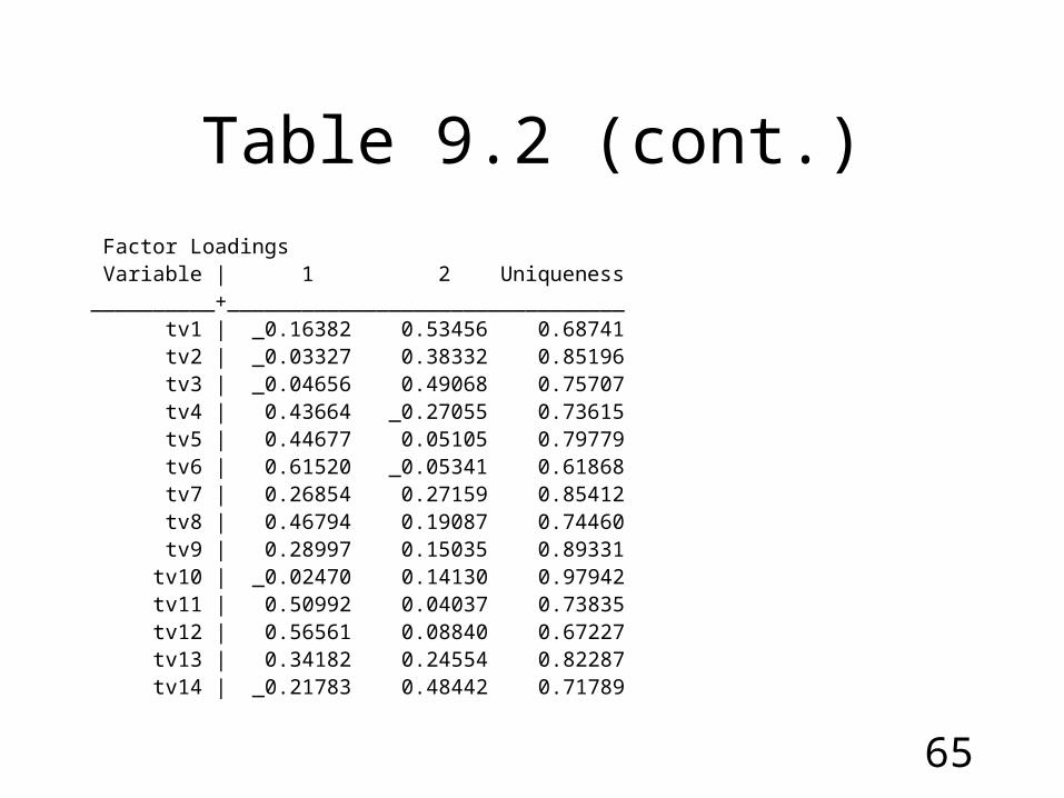
Table 9.2 (cont.)

Factor Loadings Variable | 1 2 Uniqueness__________+________________________________ tv1 | _0.16382 0.53456 0.68741 tv2 | _0.03327 0.38332 0.85196 tv3 | _0.04656 0.49068 0.75707 tv4 | 0.43664 _0.27055 0.73615 tv5 | 0.44677 0.05105 0.79779 tv6 | 0.61520 _0.05341 0.61868 tv7 | 0.26854 0.27159 0.85412 tv8 | 0.46794 0.19087 0.74460 tv9 | 0.28997 0.15035 0.89331 tv10 | _0.02470 0.14130 0.97942 tv11 | 0.50992 0.04037 0.73835 tv12 | 0.56561 0.08840 0.67227 tv13 | 0.34182 0.24554 0.82287 tv14 | _0.21783 0.48442 0.71789

66

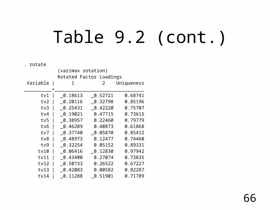
Table 9.2 (cont.). rotate (varimax rotation) Rotated Factor Loadings Variable | 1 2 Uniqueness__________+________________________________ tv1 | _0.18613 _0.52721 0.68741 tv2 | _0.20116 _0.32798 0.85196 tv3 | _0.25431 _0.42220 0.75707 tv4 | _0.19021 0.47715 0.73615 tv5 | _0.38957 0.22460 0.79779 tv6 | _0.46289 0.40873 0.61868 tv7 | _0.37740 _0.05870 0.85412 tv8 | _0.48973 0.12477 0.74460 tv9 | _0.32254 0.05152 0.89331 tv10 | _0.06416 _0.12830 0.97942 tv11 | _0.43400 0.27074 0.73835 tv12 | _0.50733 0.26522 0.67227 tv13 | _0.42083 0.00582 0.82287 tv14 | _0.11288 _0.51901 0.71789

Figure 9-2:.

TV1

TV2

TV3

TV4

TV5

TV6

TV7 TV8

TV9TV10TV11TV12

TV13

TV14

Factor 1

Factor 2

68

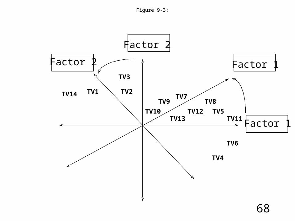
Figure 9-3:

TV1 TV2

TV3

TV4

TV5

TV6

TV7TV8TV9

TV10TV11

TV12TV13

TV14

Factor 2

Factor 2 Factor 1

Factor 1

69

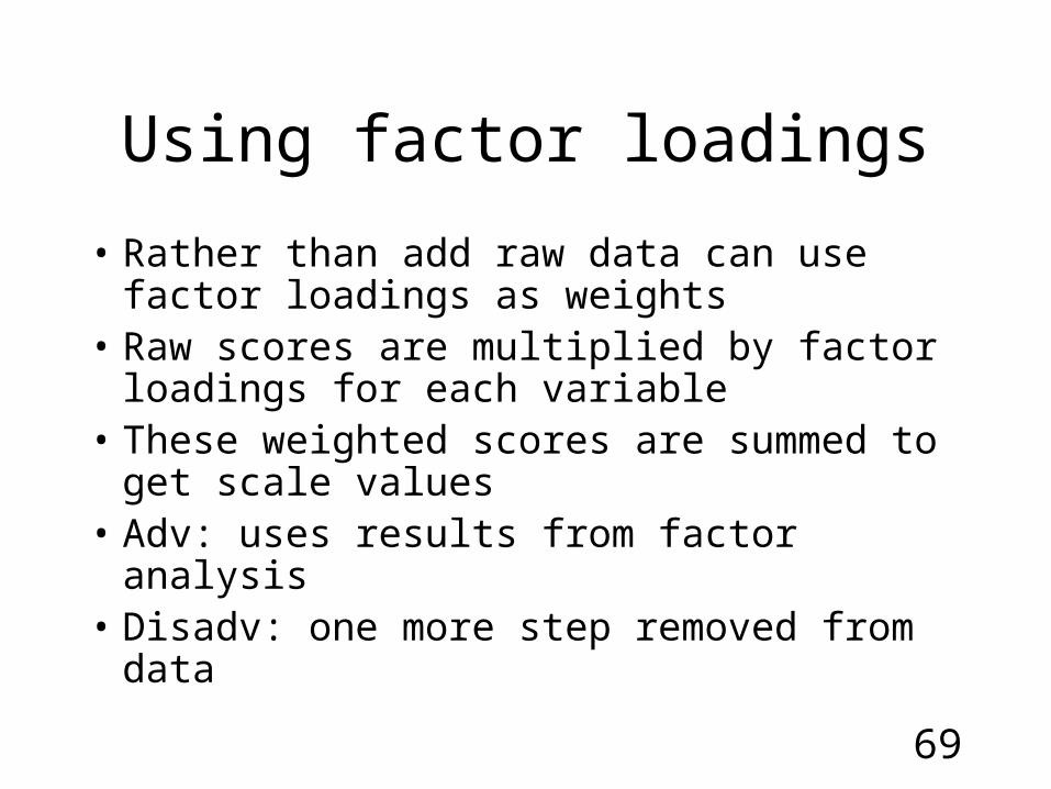
Using factor loadings

• Rather than add raw data can use factor loadings as weights

• Raw scores are multiplied by factor loadings for each variable

• These weighted scores are summed to get scale values

• Adv: uses results from factor analysis• Disadv: one more step removed from data

70

At least 3 ways to create scale

• Add items that load well on each factor

• Multiply items by factor loadings

• Explore alternative factor structures by varying parameters such as cutoff threshold, extraction method, rotation method.

Steps in the Scale Construction Process

1) Administer questions (items) to sample (using existing instrument or adaptation of old one or new one).

2) Examine univariate distribution of items and reverse code any that point in opposite direction.

3) Factor analyze scale items setting eigenvalue cut-off greater than one. Also decide on factor method, principle components, principle factors, etc.

4) Decide on rotation method: orthogonal (varimax) or oblique (promax)

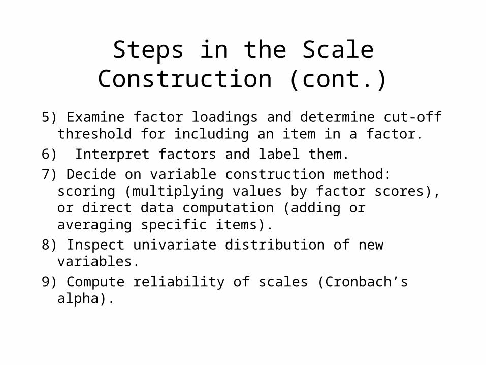
Steps in the Scale Construction (cont.)

5) Examine factor loadings and determine cut-off threshold for including an item in a factor.

6) Interpret factors and label them.

7) Decide on variable construction method: scoring (multiplying values by factor scores), or direct data computation (adding or averaging specific items).

8) Inspect univariate distribution of new variables.

9) Compute reliability of scales (Cronbach’s alpha).

73

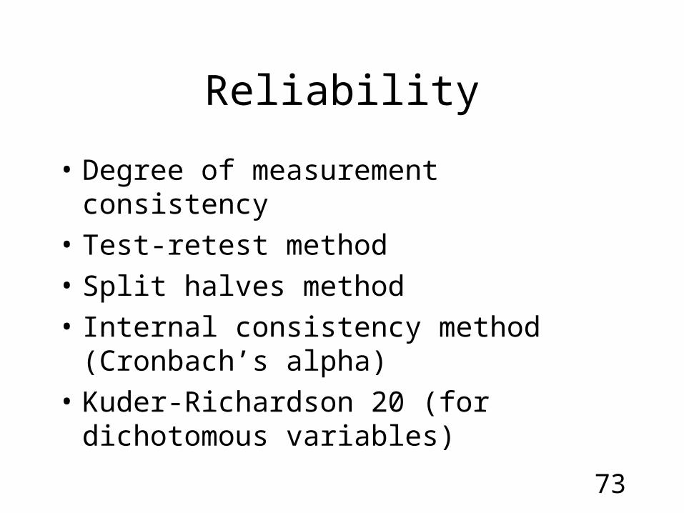
Reliability

• Degree of measurement consistency

• Test-retest method

• Split halves method

• Internal consistency method (Cronbach’s alpha)

• Kuder-Richardson 20 (for dichotomous variables)

74

Validity

• Degree instrument measures what it is intended to measure

• Criterion validity-correlation between instrument and outcome (difficult to assess)

• Content validity – degree measures all domains• Construct validity-does measure behave as

expected (e.g., smoking correlate with delinquency)

75

• Statistical analysis often seen as difficult and a barrier to quantitative evaluation

• Statistical analysis is not too hard as there are rules and procedures

• Need to know levels of measurement and the logic of hypotheses testing

• The issues is the quality of the study design and data, not the statistical analysis

Chapter 10: Statistical Analysis

76

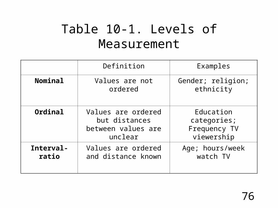
Table 10-1. Levels of Measurement

Definition Examples

Nominal Values are not ordered Gender; religion; ethnicity

Ordinal Values are ordered but distances between values are

unclear

Education categories; Frequency TV viewership

Interval-ratio Values are ordered and distance known

Age; hours/week watch TV

77

Independent, Dependent, & Mediating Variables

• Dependent variables

• Independent variables

• Moderators

• Mediators

• Not Immutable Characteristic of Variable

78

Figure 10-1 Diagram of Mediating and Moderating Variables

Z is MediatingZ is Moderating

Y Smoking

X Campaign

Z Gender

XZ InteractionY SmokingX Campaign

Z Spousal Communication

79

Statistical tests

The model status of a variable (independent or dependent), and its level of measure (nominal, ordinal or interval-ratio) determine the type of statistical test to be used to determine the strength of a relationship between two variables.

1. hypothesis testing,

2. degrees of freedom, and

3. probability.

80

1. Hypothesis Testing

An hypothesis specifies a relationship between a dependent variable and an independent variable.

For example, campaign exposure (independent variable) increases knowledge about contraceptives (dependent variable).

The goal of evaluation is often to test such hypotheses with data derived to test the effect of an intervention.

81

Hypothesis testing (cont.)

• We specify a null hypothesis which is opposite of what we wish to prove (e.g., campaign exposure does not lead to contraceptive knowledge).

• We show that null hypothesis is likely to be false – very low probability of occurring.

• Thus we have support for its opposite the research hypothesis.

82

2. Probability

• We reject null hypotheses by finding them unlikely – being in the intervention group is associated with outcome change and this association is unlikely to have occurred by chance.

• How unlikely is unlikely is unlikely enough – a less than 5% or less than 1 % occurrence

Never AlwaysHappens Happens0 -- 0.001 -- 0.01 – 0.05 – 0.10 – 0.20 ---0.50 ---- 1.0

83

3. Degrees of Freedom

• Measure of how much information is provided by the data within the context of a specific test.

• Example: 20 blue and 20 red poker chips, removing 39 of them tells you exactly which one is left.

• Degrees of freedom are often linked closely with the sample size, but may also be determined by the type of test and the distribution of the data for that test.

84

Table 10-2. Appropriate Statistical Tests as Determined by Levels of Measurement of Dependent

and Independent Variables

Independent variable

Dependent Variable

(impact scores)

Nominal Ordinal Interval Ratio

Nominal Chi-squared Chi-squared ANOVA (t-test)

Ordinal Chi-squared Chi-squared ANOVA (f-test)

Interval-ratio (Logistic regression)

(multinomial logistic regression)

Correlation

85

Association between Knowledge and Exposure

• Tables 10-3 to 10-7