1

Chapter 6 Sensitivity Analysis and Duality

PART 3Mahmut Ali GÖKÇE

2

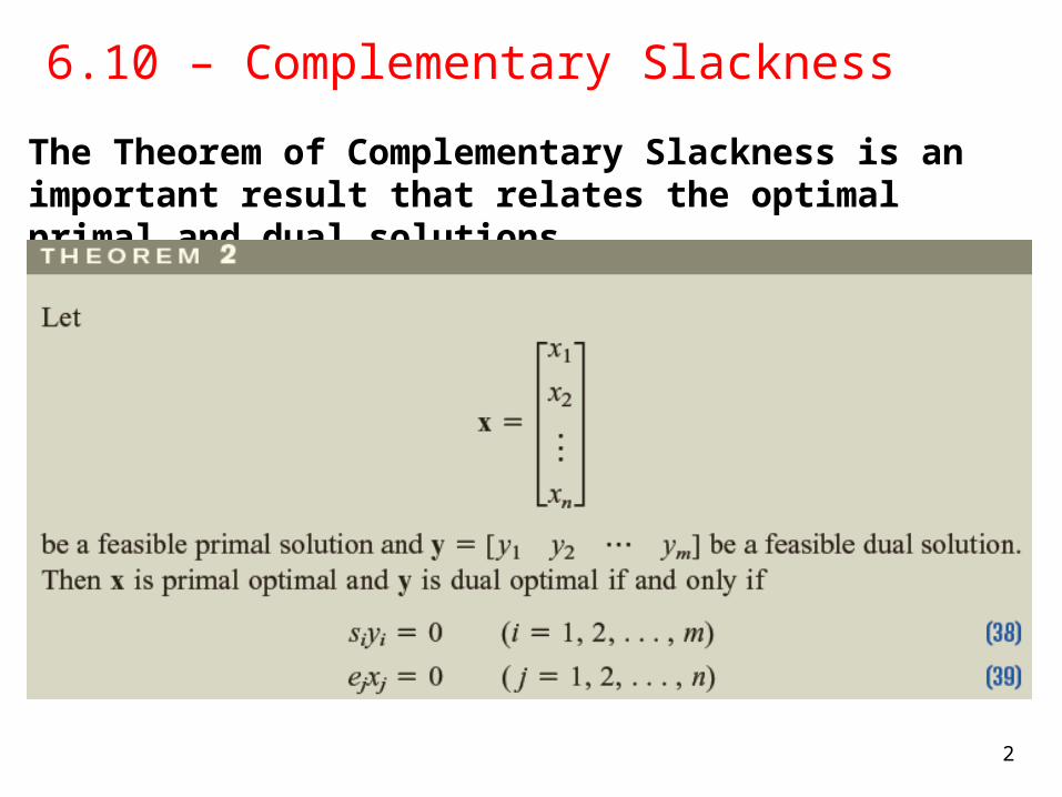
6.10 – Complementary Slackness

The Theorem of Complementary Slackness is an important result that relates the optimal primal and dual solutions.

3

6.10 – Complementary Slackness

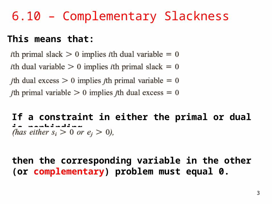
This means that:

If a constraint in either the primal or dual is nonbinding,

then the corresponding variable in the other (or complementary) problem must equal 0.

4

6.10 – Complementary Slackness

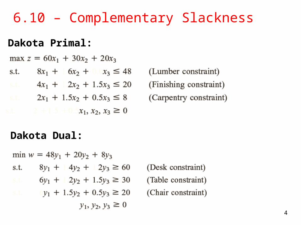
Dakota Primal:

Dakota Dual:

5

6.10 – Complementary Slackness

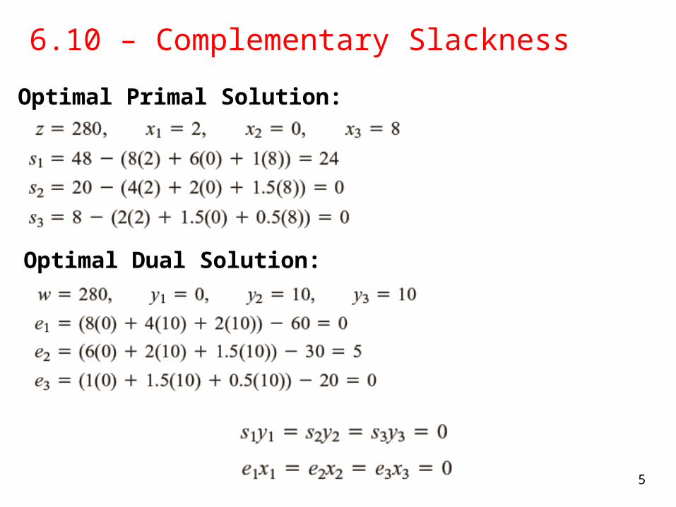
Optimal Primal Solution:

Optimal Dual Solution:

6

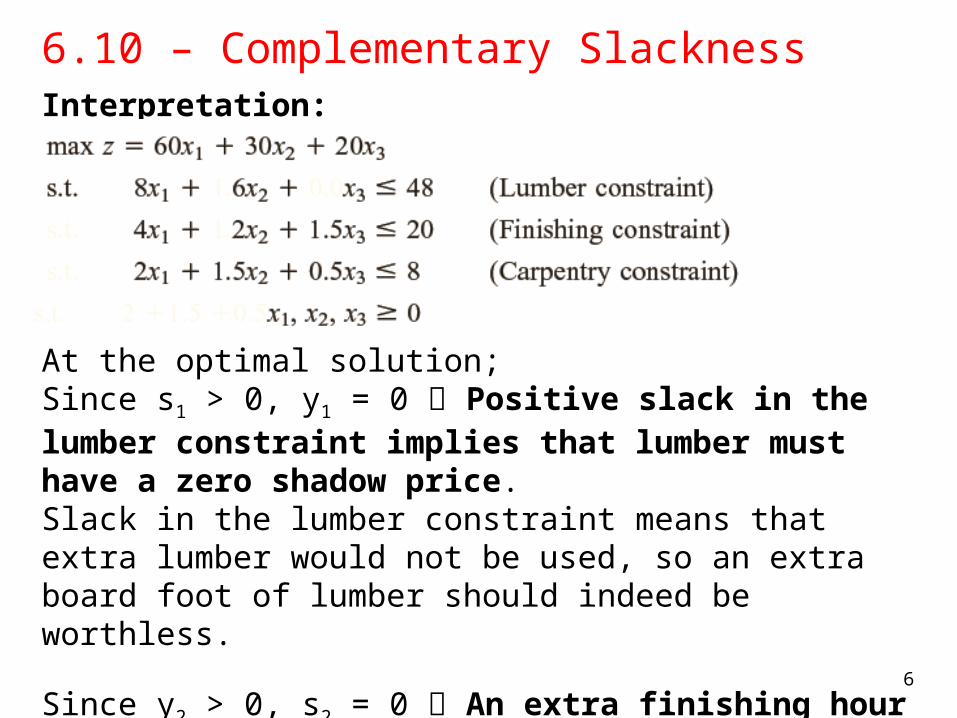
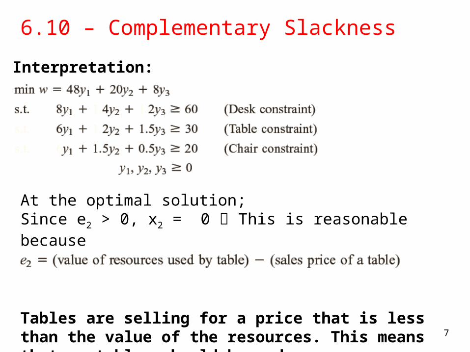
6.10 – Complementary SlacknessInterpretation:

At the optimal solution;Since s1 > 0, y1 = 0 Positive slack in the lumber constraint implies that lumber must have a zero shadow price. Slack in the lumber constraint means that extra lumber would not be used, so an extra board foot of lumber should indeed be worthless.

Since y2 > 0, s2 = 0 An extra finishing hour has some value. This can only occur if we are using all available finishing hours.

7

6.10 – Complementary Slackness

Interpretation:

At the optimal solution;Since e2 > 0, x2 = 0 This is reasonable because e2 = 6y1 + 2y2 + 1.5y3 - 30.

Tables are selling for a price that is less than the value of the resources. This means that no tables should be made.

8

6.10 – Complementary Slackness

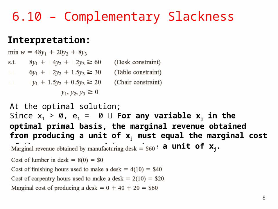
Interpretation:

At the optimal solution;Since x1 > 0, e1 = 0 For any variable xj in the optimal primal basis, the marginal revenue obtained from producing a unit of xj must equal the marginal cost of the resources used to produce a unit of xj.

9

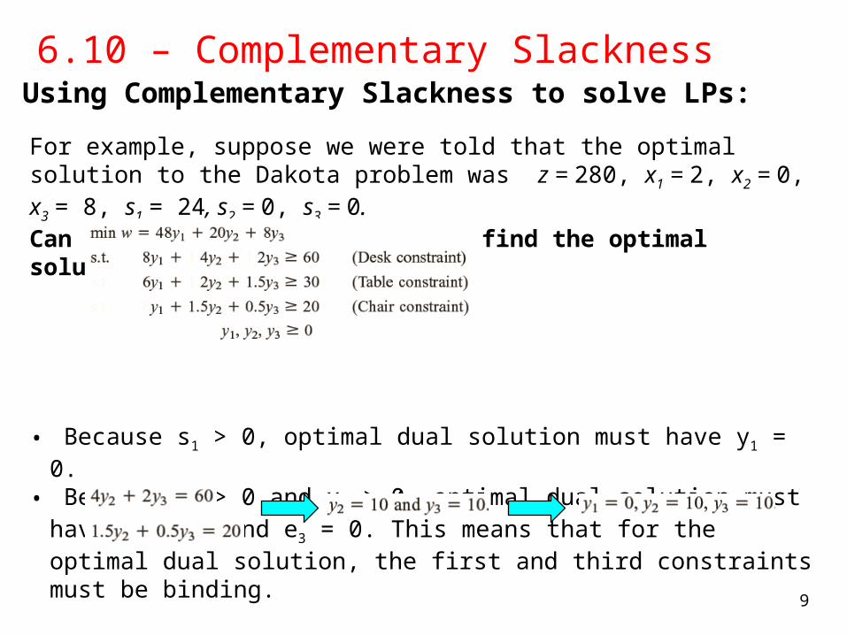
6.10 – Complementary SlacknessUsing Complementary Slackness to solve LPs:

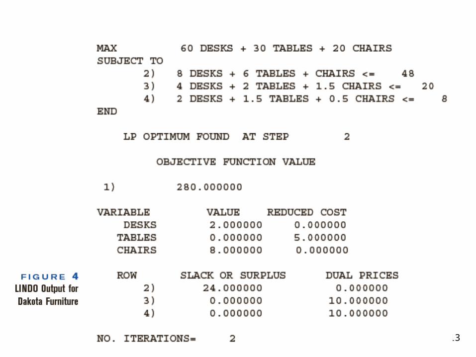
For example, suppose we were told that the optimal solution to the Dakota problem was z = 280, x1 = 2, x2 = 0, x3 = 8, s1 = 24, s2 = 0, s3 = 0.Can we use Theorem 2 to help us find the optimal solution to the Dakota dual?

• Because s1 > 0, optimal dual solution must have y1 = 0. • Because x1 > 0 and x3 > 0, optimal dual solution must have e1 = 0, and e3 = 0.

This means that for the optimal dual solution, the first and third constraints must be binding.

• From the dual theorem, we know also that z = w = 280.

10

6.8 – Shadow Prices

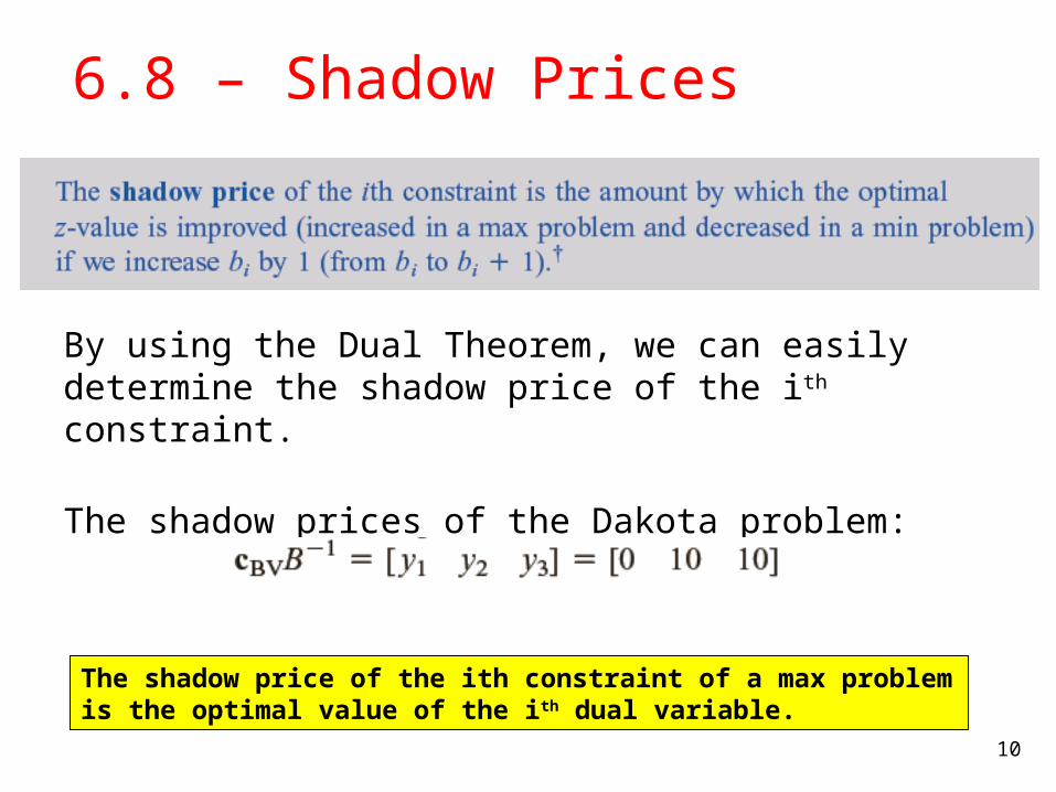
By using the Dual Theorem, we can easily determine the shadow price of the ith constraint.

The shadow prices of the Dakota problem:

The shadow price of the ith constraint of a max problem is the optimal value of the ith dual variable.

11

6.8 – Shadow Prices

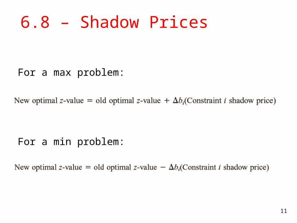
For a max problem:

For a min problem:

12

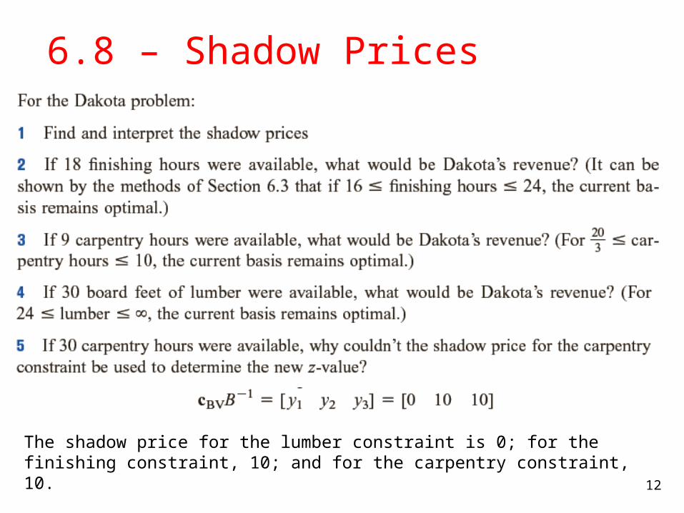
6.8 – Shadow Prices

The shadow price for the lumber constraint is 0; for the finishing constraint, 10; and for the carpentry constraint, 10.

13

14

15

6.8 – Shadow Prices

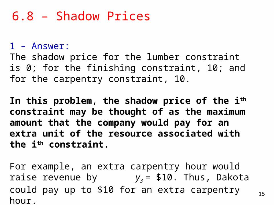
1 – Answer:The shadow price for the lumber constraint is 0; for the finishing constraint, 10; and for the carpentry constraint, 10.

In this problem, the shadow price of the ith constraint may be thought of as the maximum amount that the company would pay for an extra unit of the resource associated with the ith constraint.

For example, an extra carpentry hour would raise revenue by y3 = $10. Thus, Dakota could pay up to $10 for an extra carpentry hour.

16

6.8 – Shadow Prices

17

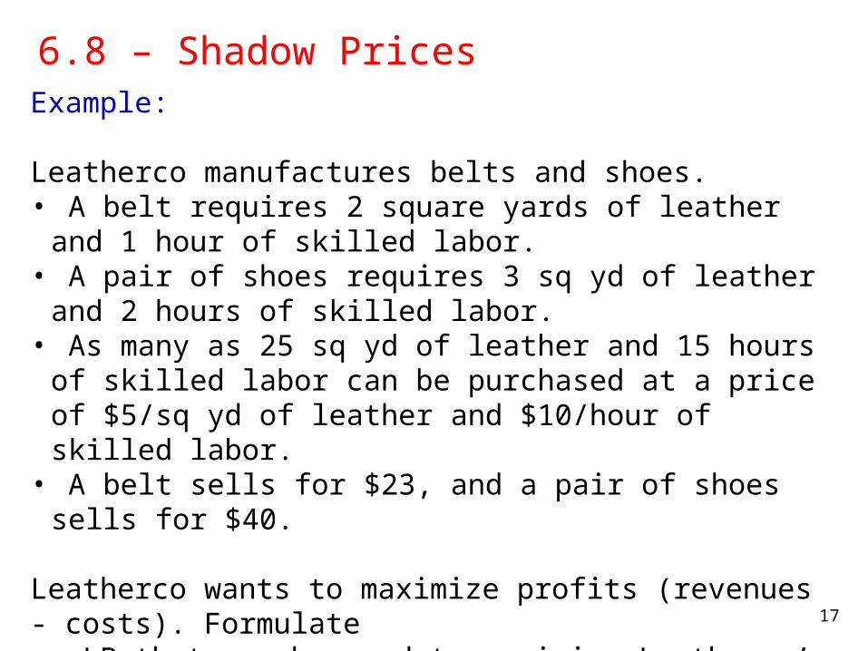
6.8 – Shadow PricesExample:

Leatherco manufactures belts and shoes. • A belt requires 2 square yards of leather and 1 hour of skilled

labor. • A pair of shoes requires 3 sq yd of leather and 2 hours of skilled

labor.• As many as 25 sq yd of leather and 15 hours of skilled labor can

be purchased at a price of $5/sq yd of leather and $10/hour of skilled labor. • A belt sells for $23, and a pair of shoes sells for $40.

Leatherco wants to maximize profits (revenues - costs). Formulatean LP that can be used to maximize Leatherco’s profits. Then find and interpret the shadow prices for this LP.

18

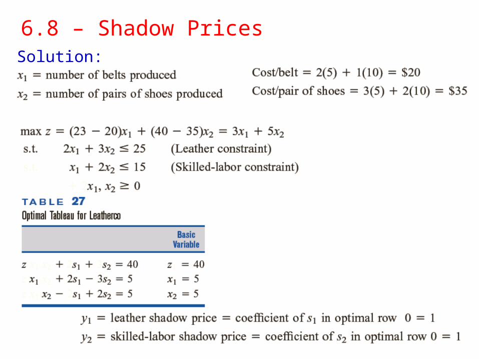
6.8 – Shadow PricesSolution:

19

6.8 – Shadow Prices (Solution cont.)

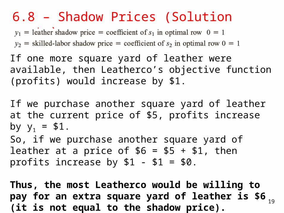
If one more square yard of leather were available, then Leatherco’s objective function (profits) would increase by $1.

If we purchase another square yard of leather at the current price of $5, profits increase by y1 = $1. So, if we purchase another square yard of leather at a price of $6 = $5 + $1, then profits increase by $1 - $1 = $0.

Thus, the most Leatherco would be willing to pay for an extra square yard of leather is $6 (it is not equal to the shadow price).

20

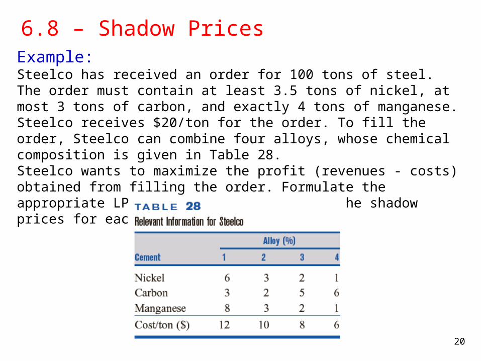
6.8 – Shadow PricesExample:Steelco has received an order for 100 tons of steel. The order must contain at least 3.5 tons of nickel, at most 3 tons of carbon, and exactly 4 tons of manganese. Steelco receives $20/ton for the order. To fill the order, Steelco can combine four alloys, whose chemical composition is given in Table 28. Steelco wants to maximize the profit (revenues - costs) obtained from filling the order. Formulate the appropriate LP. Also find and interpret the shadow prices for each constraint.

21

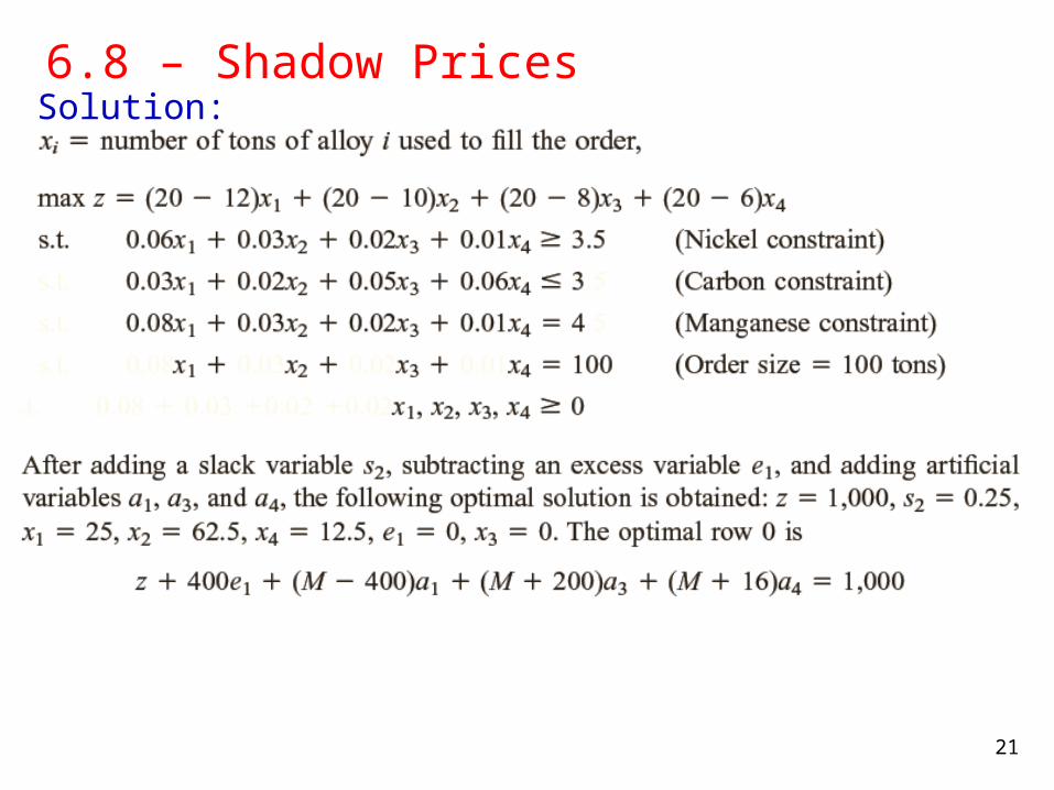
6.8 – Shadow PricesSolution:

22

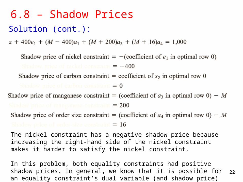
6.8 – Shadow PricesSolution (cont.):

The nickel constraint has a negative shadow price because increasing the right-hand side of the nickel constraint makes it harder to satisfy the nickel constraint.

In this problem, both equality constraints had positive shadow prices. In general, we know that it is possible for an equality constraint’s dual variable (and shadow price) to be negative.

23

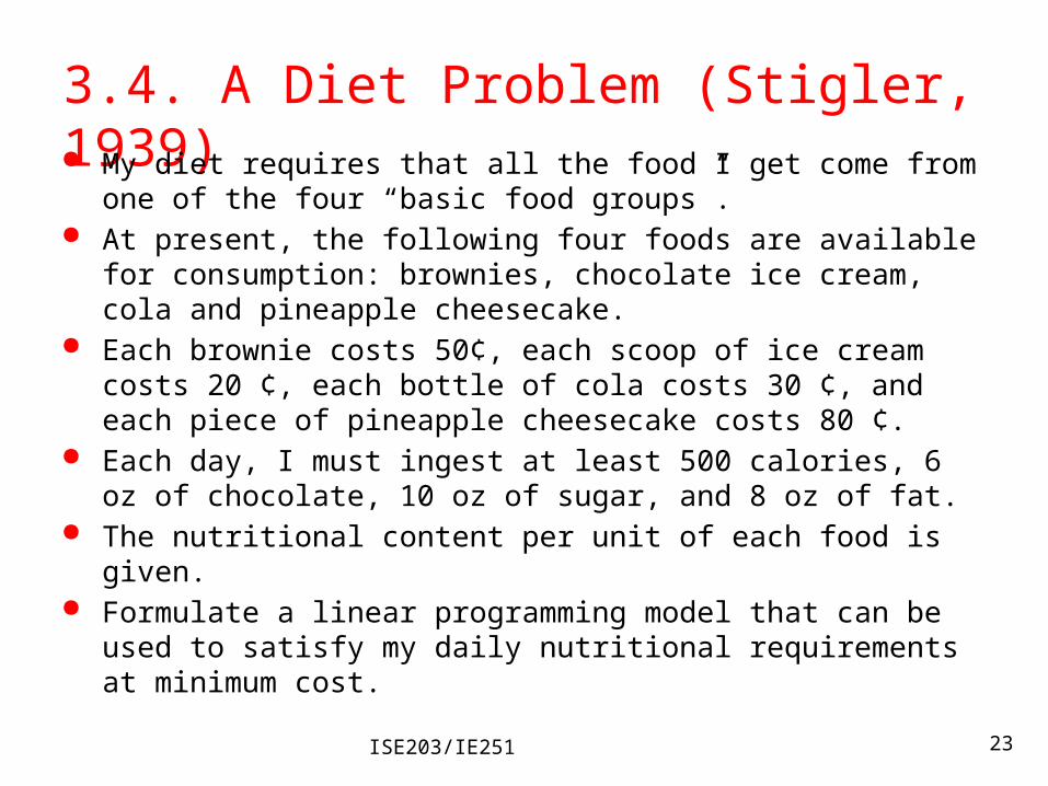
3.4. A Diet Problem (Stigler, 1939) My diet requires that all the food I get come from one of the four “basic

food groups”. At present, the following four foods are available for consumption:

brownies, chocolate ice cream, cola and pineapple cheesecake. Each brownie costs 50¢, each scoop of ice cream costs 20 ¢, each bottle of

cola costs 30 ¢, and each piece of pineapple cheesecake costs 80 ¢. Each day, I must ingest at least 500 calories, 6 oz of chocolate, 10 oz of

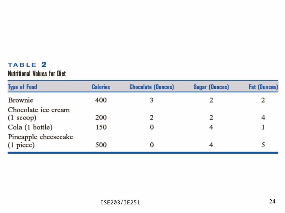
sugar, and 8 oz of fat. The nutritional content per unit of each food is given. Formulate a linear programming model that can be used to satisfy my

daily nutritional requirements at minimum cost.

ISE203/IE251

24ISE203/IE251

25

26

27

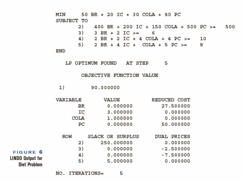
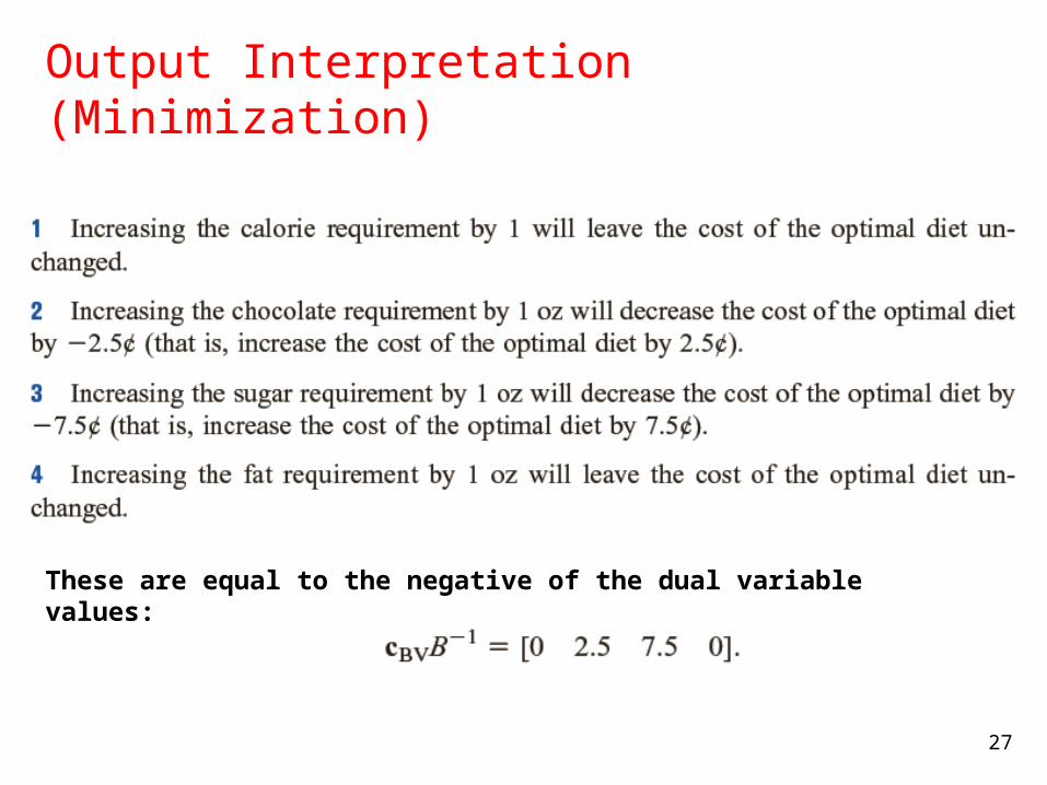
Output Interpretation (Minimization)

These are equal to the negative of the dual variable values: