Embed Size (px)
Citation preview

1
CE 530 Molecular Simulation
Lecture 15
Long-range forces and Ewald sum
David A. Kofke
Department of Chemical Engineering
SUNY Buffalo

2
Review
Intermolecular forces arise from quantum mechanics• too complex to include in lengthy simulations of bulk phases
Empirical forms give simple formulas to approximate behavior• intramolecular forms: bend, stretch, torsion
• intermolecular: van der Waals, electrostatics, polarization
Unlike-atom interactions weak link in quantitative work

3
Truncating the Potential Bulk system modeled via
periodic boundary condition• not feasible to include
interactions with all images
• must truncate potential at half the box length (at most) to have all separations treated consistently
Contributions from distant separations may be important
These two are same distance from central atom, yet:
Black atom interactsGreen atom does not
These two are nearest images for central atom
Only interactions considered

4
Truncating the Potential
Potential truncation introduces discontinuity• Corresponds to an infinite force
• Problematic for MD simulationsruins energy conservation
Shifted potentials• Removes infinite force
• Still discontinuity in force
Shifted-force potentials• Routinely used in MD
For quantitative work need to re-introduce long-range interactions
( ) ( )( )
0c c
sc
u r u r r ru r
r r
( ) ( ) ( )( )
0
c c csf
c
duu r u r r r r r
u r drr r

5
Truncating the Potential
( ) ( )( )
0c c
sc
u r u r r ru r
r r
( ) ( ) ( )( )
0
c c csf
c
duu r u r r r r r
u r drr r
Lennard-Jones example• rc = 2.5
-2.5
-2.0
-1.5
-1.0
-0.5
0.0
0.5
1.0
2.42.01.61.2Separation, r/
-0.20
-0.15
-0.10
-0.05
0.00
2.52.42.32.22.12.0Separation, r/
u(r) f(r) u(r) u-Shift u(r) f-Shift f(r) f-Shift

6
Radial Distribution Function
Radial distribution function, g(r)• key quantity in statistical mechanics
• quantifies correlation between atom pairs
Definition
Here’s an applet that computes g(r)
( )( )
( )id
r dg r
r d
r
r
Number of atoms at r for ideal gas
Number of atoms at r in actual system
( )id Nr d d
V r r
dr
4
3
2
1
0
543210
Hard-sphere g(r) Low density High density
7
Radial Distribution Function. API
U ser 's P ers pe ctiv e o n the M o lec u la r S im u la tion A P I
S pa ce
In te gra to r
C on tro lle r
M e te rR D F
M e te rFu n ction
M e te rA b s tra ct B ou nda ry C on fig u ra tion
P ha se S p ec ies P o te n tia l D isp lay D ev ice
S im u la tion

8
Radial Distribution Function. Java Code
/** * Computes RDF for the current configuration */public double[] currentValue() { iterator.reset(); //prepare iterator of atom pairs for(int i=0; i<nPoints; i++) {y[i] = 0.0;} //zero histogram while(iterator.hasNext()) { //loop over all pairs in phase double r = Math.sqrt(iterator.next().r2()); //get pair separation if(r < xMax) { int index = (int)(r/delr); //determine histogram index y[index]+=2; //add once for each atom } } int n = phase.atomCount(); //compute normalization: divide by double norm = n*n/phase.volume(); //n, and density*(volume of shell) for(int i=0; i<nPoints; i++) {y[i] /= (norm*vShell[i]);} return y;}
public class MeterRDF extends MeterFunction
9
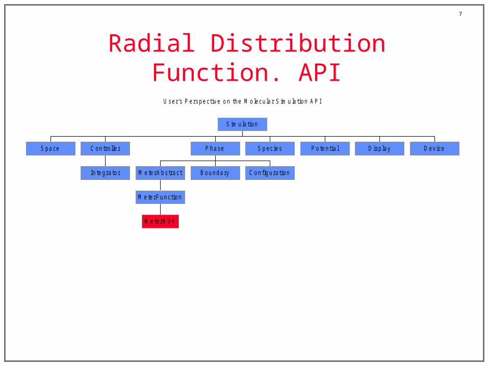
Simple Long-Range Correction
Approximate distant interactions by assuming uniform distribution beyond cutoff: g(r) = 1 r > rcut
Corrections to thermodynamic properties• Internal energy
• Virial
• Chemical potential
2( )42
cut
lrcr
NU u r r dr
Expression for Lennard-Jones model
2 214
6cut
lrcr
duP r r dr
dr
2( )4 2
cut
lrclrc
r
Uu r r dr
N
9 338
39
LJlrc
c cU N
r r
9 32 332 3
9 2LJ
lrcc c
Pr r
For rc/ = 2.5, these are about 5-10% of the total values

10
Coulombic Long-Range Correction Coulombic interactions must be treated specially
• very long range
• 1/r form does not die off as quickly as volume grows
• finite only because + and – contributions cancel
Methods• Full lattice sum
Here is an applet demonstrating direct approach
Ewald sum
• Treat surroundings as dielectric continuum
1.5
1.0
0.5
0.0
-0.5
-1.0
4321
Lennard-Jones Coulomb
214
cr
r drr

11
Aside: Fourier Series
Consider periodic function on -L/2, +L/2
A Fourier series provides an equivalent representation of the function
The coefficients are
f(x)
x/ 2L / 2L
One period
102
1
( ) cos sinn nn
f x a a nx b nx
/ 21
/ 2
1
( )cos(2 / )
( )sin(2 / )
L
n LL
L
n LL
a f x nx L dx
b f x nx L dx

12
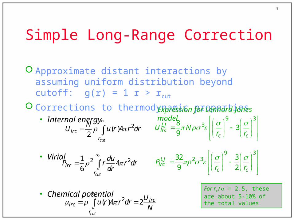
Fourier Series Example
f(x) is a square wave
/ 21
/ 2
0 / 21 1
/ 2 0
/ 21
/ 2
4
( )cos(2 / )
cos(2 / ) cos(2 / ) 0
( )sin(2 / )
n odd
0 n even
L
n LL
L
L LL
L
n LL
n
a f x nx L dx
nx L dx nx L dx
b f x nx L dx
f(x)
x

13
Fourier Series Example
f(x) is a square wave
/ 21
/ 2
0 / 21 1
/ 2 0
/ 21
/ 2
4
( )cos(2 / )
cos(2 / ) cos(2 / ) 0
( )sin(2 / )
n odd
0 n even
L
n LL
L
L LL
L
n LL
n
a f x nx L dx
nx L dx nx L dx
b f x nx L dx
f(x)
x
n = 1
14
Fourier Series Example
f(x) is a square wave
/ 21
/ 2
0 / 21 1
/ 2 0
/ 21
/ 2
4
( )cos(2 / )
cos(2 / ) cos(2 / ) 0
( )sin(2 / )
n odd
0 n even
L
n LL
L
L LL
L
n LL
n
a f x nx L dx
nx L dx nx L dx
b f x nx L dx
f(x)
x
n = 1, 3

15
Fourier Series Example
f(x) is a square wave
/ 21
/ 2
0 / 21 1
/ 2 0
/ 21
/ 2
4
( )cos(2 / )
cos(2 / ) cos(2 / ) 0
( )sin(2 / )
n odd
0 n even
L
n LL
L
L LL
L
n LL
n
a f x nx L dx
nx L dx nx L dx
b f x nx L dx
f(x)
x
n = 1, 3, 5

16
Fourier Series Example
f(x) is a square wave
/ 21
/ 2
0 / 21 1
/ 2 0
/ 21
/ 2
4
( )cos(2 / )
cos(2 / ) cos(2 / ) 0
( )sin(2 / )
n odd
0 n even
L
n LL
L
L LL
L
n LL
n
a f x nx L dx
nx L dx nx L dx
b f x nx L dx
f(x)
x
n = 1, 3, 5, 7

17
Fourier Representation
The set of Fourier-space coefficients bn contain complete information about the function
Although f(x) is periodic to infinity, bn is non-negligible over only a finite range
Sometimes the Fourier representation is more convenient to use1.2
1.0
0.8
0.6
0.4
0.2
bn
403020100
n

18
Convergence of Fourier Sum
If f(x) = sin(2kx/L), transform is simple• bn = 1 for n = k
• bn = 0 otherwise
f(x)
x
1.0
0.8
0.6
0.4
0.2
0.0
bn
403020100
n
Converges very quickly!

19
Observations on Fourier Sum
Smooth functions f(x) require few coefficients bn
Sharp functions (square wave) require more coefficients Large-n coefficients describe high-frequency behavior of f(x)
• large n = short wavelength
Small-n coefficients describe low-frequency behavior• small n = long wavelength
• e.g., n = 0 coefficient is simple average of f(x)

20
Fourier Transform As L increases, f(x) becomes less periodic Fourier transform arrives in limit of L Compact form obtained with exponential form of cos/sin
Useful relations• derivative
• convolution
2 2102
1
( ) cos sinnx nxn nL L
n
f x a a b
/ 21
/ 2
1
( )cos(2 / )
( )sin(2 / )
L
nL
L
nL
a f x nx L dx
b f x nx L dx
2ˆ( ) ( ) ikxf x f k e dk
2ˆ ( ) ( ) ikxf k f x e dx
inverse
forward
cos sinie i
an = real part of transform
bn = imaginary part
( ) ˆ( ) ( ) ( 2 ) ( )m mf x k ik f k ˆ ˆ( ) ( ) ( ) ( ) ( )f t g x t dt k f k g k

21
Fourier Transform Example Gaussian
Transform is also a Gaussian!
Width of transform is reciprocal of width of function• k-space is “reciprocal” space
• sharp f(x) requires more values of F(k) for good representation
• (x-xo) transforms into a sine/cosine wave of frequency xo:
1/ 2 22 1ˆ( ) exp2
kf k
2
( ) exp2 2
xf x
f(x)
x
F(k)
x
2ˆ( ) oikxk e

22
Fourier Transform Relevance
Many features of statistical-mechanical systems are described in k-space• structure
• transport behavior
• electrostatics
This description focuses on the correlations shown over a particular length scale (depending on k)
Macroscopic observables are recovered in the k 0 limit Corresponding treatment is applied in the time/frequency
domains
23
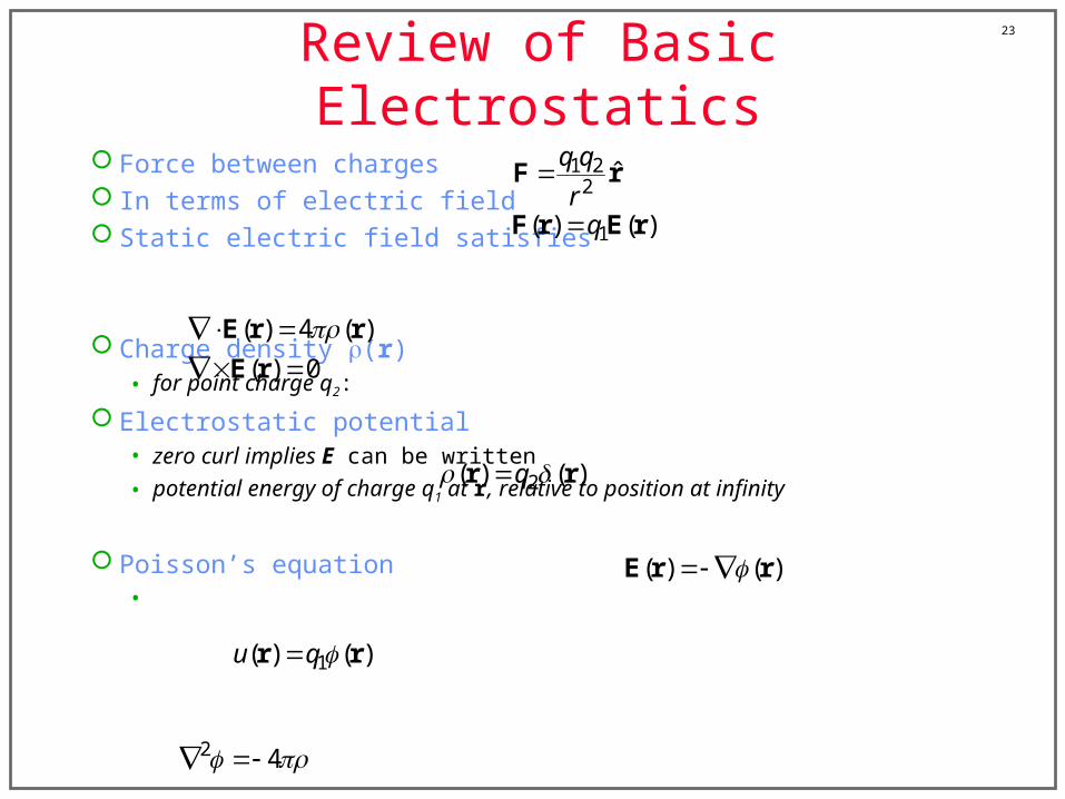
Review of Basic Electrostatics
Force between charges In terms of electric field Static electric field satisfies
Charge density (r)• for point charge q2:
Electrostatic potential• zero curl implies E can be written
• potential energy of charge q1 at r, relative to position at infinity
Poisson’s equation•
1 22
ˆq q
rF r
1( ) ( )qF r E r
( ) 4 ( )
( ) 0
E r r
E r
2( ) ( )q r r
( ) ( ) E r r
2 4
1( ) ( )u q r r
24
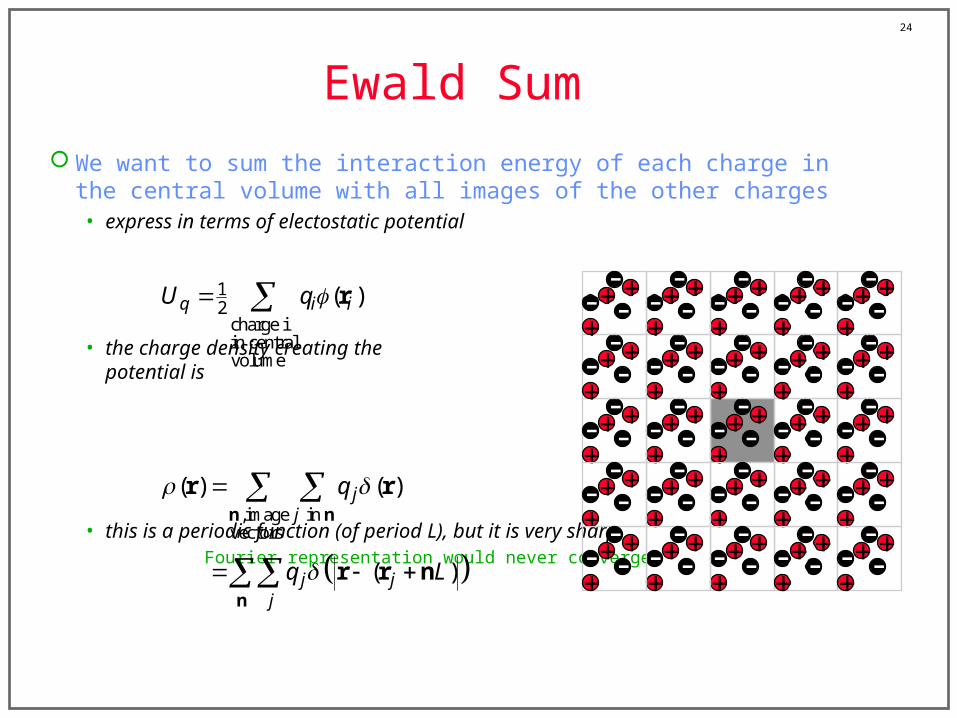
Ewald Sum
We want to sum the interaction energy of each charge in the central volume with all images of the other charges• express in terms of electostatic potential
• the charge density creating the potential is
• this is a periodic function (of period L), but it is very sharpFourier representation would never converge
+ ++
--
-+ ++
--
- + ++
--
-+ ++
--
- + ++
--
-
+ ++
--
-+ ++
--
- + ++
--
-+ ++
--
- + ++
--
-
+ ++
--
-+ ++
--
- + ++
--
-+ ++
--
- + ++
--
-
+ ++
--
-+ ++
--
- + ++
--
-+ ++
--
- + ++
--
-
+ ++
--
-+ ++
--
- + ++
--
-+ ++
--
- + ++
--
-12
charge iin centralvolume
( )q i iU q r
,image in
vectors
( ) ( )
( )
jj
j jj
q
q L
n n
n
r r
r r n

25
Ewald Sum: Fourier 1.
Compute field instead by smearing all the charges
Electrostatic potential via Poisson equation• direct space form
• reciprocal space
Fourier transform the charge density
23/ 2( ) ( / ) exp ( )j jj
q L n
r r r n
include n = 0
2 ( ) 4 ( ) r r2 ( ) 4 ( )k k k
/ 21
/ 2
1
( )cos(2 / )
( )sin(2 / )
L
n LL
L
n LL
a f x nx L dx
b f x nx L dx
2
1
/ 41
( ) ( )
j
iV
V
i kjV
j
d e
q e e
k r
k r
k r r
Large takes back to function

26
Ewald Sum. Fourier 2.
Use Poisson’s equation for electrostatic potential
Invert transform to recover real-space potential
• in principle requires sum over infinite number of wave vectors k
• but reciprocal Gaussian goes to zero quickly if is small
102
1
( ) cos sinn n
n
f x a a nx b nx
2
4( ) ( )
k
k k
2
0
( ) / 42
0
( ) ( )
41 j
i
k
ij k
k j
e
qe e
V k
k r
k r r
r k

27
Ewald Sum. Fourier 3.
The electrostatic energy can now be obtained• for point charges in potential of smeared charges
Two corrections are needed• self interaction
• correct for smearing
2
2
12
( )/ 412 2 2
0 ,
2/ 412 2
0
( )
4
4( )
i j
q i ii
ii jk
i j
k
U q
q qVe e
k V
Ve
k
k r r
k
k
r
k
product of identical sums
1( ) ji
jj
q eV
k rk

28
Ewald Sum. Self Interaction 1. In Ewald sum, each point charge is replaced by smeared Gaussian centered on
that charge• this is done to estimate the electrostatic potential field
All point charges interact with the resulting field to yield the potential energy• This means that the point charge
interacts with its smeared representation
• We need to subtract this
x
x
x

29
Ewald Sum. Self Interaction 2. We work in real space to deal with the self term
• Poisson’s equation for the electrostatic potential due to a single smeared charge
• The solution is
• In particular, at r = 0
• The self-correction subtracts this for each charge
2 ( ) 4 ( ) r r23/ 2( ) ( / ) expj jq
r r r
( ) jqr erf r
r
1/ 2(0) 2 ( / )jq
1
2
12
2
(0)self jj
jj
U q
q
independent of configuration
2 22
1r
r rr

30
Ewald Sum. Smearing Correction 1.
We add the correct field and subtract the approximate one to correct for the smearing
This field is short ranged for large (narrow Gaussians)• can view as point charges surrounded by shielding
countercharge distribution
( ) ( ) ( )p Gj jj
j jj
j j
jj
j
q qerf
qerfc
r r r
r rr r r r
r rr r
x

31
Ewald Sum. Smearing Correction 2.
Sum interaction of all charges with field correction• convenient to stay in real space
• usually is chosen so that sum converges within central image
Total Coulomb energy
• each term depends on , but the sum is independent of itif enough lattice vectors are used in the reciprocal- and real-space sums
Here is an applet that demonstrate the Ewald method
12
12
( )i j iji j
i jij
iji j
U q r
q qerfc r
r
n
n
( ) ) )c q selfU U U U

32
Ewald Method. Comments
Basic form requires an O(N2) calculation• efficiency can be introduced to reduce to O(N3/2)
• good value of is 5L, but should check for given application
• can be extended to sum point dipoles
Other methods are in common use• reaction field
• particle-particle/particle mesh
• fast multipole

33
Summary
Contributions from distant interactions cannot be neglected• potential truncated at no more than half box length
• treat long-range assuming uniform radial distribution function
Coulombic interactions require explicit summing of images• too costly to perform direct sum
• Ewald method is more efficientsmear charges to approximate electrostatic field
simple correction for self interaction
real-space correction for smearing