1

AUV Navigation and Localization - A ReviewLiam Paull, Sajad Saeedi, Mae Seto and Howard Li

Abstract

Autonomous underwater vehicle (AUV) navigation and localization in underwater environments is particularlychallenging due to the rapid attenuation of GPS and radio frequency signals. Underwater communications are lowbandwidth and unreliable and there is no access to a global positioning system. Past approaches to solve the AUVlocalization problem have employed expensive inertial sensors, used installed beacons in the region of interest, orrequired periodic surfacing of the AUV. While these methodsare useful, their performance is fundamentally limited.Advances in underwater communications and the applicationof simultaneous localization and mapping (SLAM)technology to the underwater realm have yielded new possibilities in the field.

This paper presents a review of the state of the art of underwater autonomous vehicle navigation and localization,as well as a description of some of the more commonly used methods. In addition, we highlight areas of futureresearch potential.

I. INTRODUCTION

The development of autonomous underwater vehicles (AUVs) began in earnest in the 1970s. Since then, ad-vancements in the efficiency, size, and memory capacity of computers have enhanced that potential. As a result,many tasks that were originally achieved with towed arrays or manned vehicles are being completely automated.AUV designs include torpedo-like, gliders, and hovering, and their sizes range from human-portable to hundredsof tons.

AUVs are now being used for a variety of tasks, including oceanographic surveys, demining, and bathymetricdata collection in marine and riverine environments. Accurate localization and navigation is essential to ensure theaccuracy of the gathered data for these applications.

A distinction should be made between navigation and localization. Navigational accuracy is the precision withwhich the AUV guides itself from one point to another. Localization accuracy is the error in how well the AUVlocalizes itself within a map.

AUV navigation and localization is a challenging problem due primarily to the rapid attenuation of higher fre-quency signals and the unstructured nature of the undersea environment. Above water, most autonomous systems relyon radio or spread spectrum communications and global positioning. However, underwater such signals propagateonly short distances and acoustic based sensors and communications perform better. Acoustic communications stillsuffer from many shortcomings such as:

• Small bandwidth, which means communicating nodes have had to use time division multiple access (TDMA)techniques to share information,

• Low data rate, which generally constrains the amount of datathat can be transmitted,• High latency since the speed of sound in water is only 1500m/s(slow compared with the speed of light),• Variable sound speed due to fluctuating water temperature and salinity,• Multi-path transmissions due to the presence of an upper (free surface) and lower (sea bottom) boundary

coupled with highly variable sound speed• Unreliability, resulting in the need for a communications system designed to handle frequent data loss in

transmissions.

Liam Paull is a COBRA team member with the Department of Electrical and Computer Engineering, University of New Brunswick,Fredericton, Canada,liam.paull@unb.ca

Sajad Saeedi G. is a COBRA team member with the Department of Electrical and Computer Engineering, University of New Brunswick,Fredericton, Canada,sajad.saeedi.g@unb.ca

Mae Seto is with Defence Research and Development Canada, Halifax, Nova Scotia, Canada,Mae.Seto@drdc-rddc.gc.caHoward Li is a COBRA team member with the Department of Electrical and Computer Engineering, University of New Brunswick,

Fredericton, Canada,howard@unb.ca

2

Notwithstanding these significant challenges, research inAUV navigation and localization has exploded in thelast ten years. The field is in the midst of a paradigm shift from old technologies, such as long baseline (LBL)and ultra short baseline (USBL), which require pre-deployed and localized infrastructure, towards dynamic multi-agent system approaches that allow for rapid deployment andflexibility with minimal infrastructure. In addition,simultaneous localization and mapping (SLAM) techniques developed for above ground robotics applications arebeing increasingly applied to underwater systems. The result is that bounded error and accurate navigation forAUVs is becoming possible with less cost and overhead.

A. Outline

AUV navigation and localization techniques can be categorized according to Fig. 1. This review paper will beorganized based on this structure.

acoustic

transponders

and modems

acoustic

modem

manned surface

supporthomogeneous

teams

heterogeneous

teams

inertial / dead reckoning

AUV Navigation

imaging

sonar

ranging

sonar

SONAR

Sensor Technology

Collaboration

magneticacousticoptical

Geophysical

Sensor Hardware

magnetometer

Cameras

monocular stereo

Transponders

long

baseline /

GIBs

ultra-short

baseline

single fixed

beacon

IMUpressure

sensor

autonomous

surface crafts

Cooperative Localization

DVLcompass

short

baseline

Fig. 1. Outline of underwater navigation classifications. These methods are often combined in one system to provide increased performance.

In general, these techniques fall into one of three main categories:• Inertial / Dead Reckoning: Inertial navigation uses accelerometers and gyroscopes for increased accuracy to

propagate the current state. Nevertheless, all of the methods in this category have position error growth thatis unbounded.

• Acoustic transponders and modems: Techniques in this category are based on measuring the time-of-flight(TOF) of signals from acoustic beacons or modems to perform navigation.

• Geophysical: Techniques that use external environmental information as references for navigation. This must bedone with sensors and processing that are capable of detecting, identifying, and classifying some environmentalfeatures.

Sonar sensors are based on acoustic signals, however, navigation with imaging or bathymetric sonars are based ondetection, identification, and classification of features in the environment. Therefore, navigation that is sonar-based

3

falls into both the acoustic and geophysical categories. A distinction is made between sonar and other acoustic basednavigation schemes, which rely on externally generated acoustic signals emitted from beacons or other vehicles.

The type of navigation system used is highly dependent on thetype of operation or mission and that in manycases different systems can be combined to yield increased performance. The most important considerations arethe size of the region of interest and the desired localization accuracy.

Past reviews on this topic include [1], [2], and [3]. Significant advances have been made since these reviews bothin previously established technologies, and in new areas. In particular, the development of acoustic communicationsthrough the use of underwater modems has lead to the development of new algorithms. In addition, advancementsin SLAM research has been applied to the underwater domain ina number of new ways.

II. BACKGROUND

Most modern systems process and filter the data from the sensors to derive a coherent, recursive estimate of theAUV pose. This section will review some of the most common underwater sensors, popular state estimation filters,the basics of SLAM, and the foundations of cooperative navigation.

A. Commonly Used Underwater Navigation Sensors

Tables I-V describe some commonly used sensors for underwater navigation.

Description Performance CostA compass provides a globally bounded heading reference. A typical magneticcompass does so by measuring the magnetic field vector. This type of compassis subject to bias in the presence of objects with a strong magnetic signature andpoints to the earth’s magnetic north pole. More common in marine applications,a gyrocompass measures heading using a fast spinning disc and the rotationof the earth. It is unaffected by metallic objects and pointsto true north.

Accuracywithin 1o

to 2o fora modestlypriced unit.

On the orderof hundredsof dollarsUS.

TABLE ICOMPASS

Description Performance CostUnderwater depth can be measuredwith a barometer or pressure sen-sor.

Since the pressure gradient is much steeper underwater(10m = 1 atmosphere) we can achieve high accuracy≈0.1m.

≈ $100 −200USD

TABLE IIPRESSURESENSOR

Description Performance CostThe DVL uses acoustic measurements to capture bottom tracking anddetermine the velocity vector of an AUV moving across the seabed. Itdetermines the AUV surge, sway, and heave velocities by transmittingacoustic pulses and measuring the Doppler shifted returns from these pulsesoff the seabed. DVLs will typically consist of 4 or more beams. 3 beamsare needed to obtain a 3D velocity vector .

Nominalstandarddeviation onthe order of0.3cm/s-0.8cm/s.

≈ $20k - 80kUSD

TABLE IIIDOPPLERVELOCITY LOG

4

Description Performance CostA sonar is a device for remotely detecting andlocating objects in water using sound. Passivesonars are listening devices that record thesounds emitted by objects in water. Activesonars are devices that produce sound wavesof specific, controlled frequencies, and listenfor the echoes of these emitted sounds returnedfrom remote objects in the water. Active sonarscan be categorized as either imaging sonarsthat produce an image of the seabed, or rang-ing sonars which produce bathymetric maps.More details of specific active sonar devicesare presented in Table IV in Sec. V-B.

Along-track image resolution for an imagingside-scan sonar is a function of many factorssuch as range, sonar frequency, and water con-ditions, however cross-track resolution is inde-pendent of range. For example, a Klein 5000side-scan operating at 455kHz can achieve analong track resolution of 10cm at 38m rangeand 61cm at the maximum 250m range and aKlein 5900 sidescan operating at 600kHz canachieve along track resolution 5cm at 10m and20cm resolution at the maximum 100m range.In both cases nominal cross-track resolution is3.75cm Resolution for a bathymetry sonar ison the order of≈ 0.4o − 2o along track and≈ 5− 10cm cross track [4].

Prices varywidely from$20k −200kUSD ormore. [4]

TABLE IVSONAR

Description Performance CostGlobal PositioningSystems can be usedfor surface vehicles.Position is estimatedusing the time-of-flight of signals fromsynchronized satellites.

Many factors can influence the accuracy of a GPS reading, includingtype of GPS technique used, atmospheric conditions, numberofsatellites in view, and others. Precisions for different GPS systems are:common commercial off-the-shelf GPS - 10m, Wide Area DifferentialGPS (WADGPS) - 0.3-2m, Real-Time Kinematic (RTK) - 0.05-0.5m,Post processed - 0.02 - 0.25m.

Fromhundredsto thousandsof dollars.

TABLE VGLOBAL POSITIONING SYSTEM

B. State Estimation

The basis of any navigation algorithm is state estimation.Consider a robot whose pose at timet is given byxt.The goal of recursive state estimation is to estimate the belief distribution of the statext denoted bybel(xt)

given by:

bel(xt) = p(xt|u1:t, z1:t) (1)

whereu is some control input or odometry andz is a measurement used for localization.The propagation of the state is given by some general non-linear process equation:

xt = f(xt−1, ut, ǫt) (2)

whereǫt is process noise. The state is observable through some measurement function:

zt = h(xt, δt), (3)

whereδt is measurement noise. Typically, the state at timet is recursively estimated through an approximation ofthe Bayes’ filter which operates in a predict-update cycle. Prediction is given by [6]:

bel(xt) =∑

xt−1

p(xt|xt−1, ut)bel(xt−1) (4)

5

Description Performance CostUse a combination of accelerometers and gyroscopes (and sometimes magne-tometers) to estimate a vehicle’s orientation, velocity, and gravitational forces.

• Gyroscope: Measures angular rates. For underwater applications, the follow-ing two categories are widely used:

– Ring Laser / Fibre Optic: Light is passed either through a series ofmirrors (ring laser) or fibre optic cable in different directions. Theangular rates are determined based on the phase change of thelightafter passing through the mirrors or fibre.

– MEMS: An oscillating mass is suspended within a spring system.Rotation of the gyroscope results in a perpendicular Coriolis force onthe mass which can be used to calculate the angular rate of sensor.

Since a gyroscope measures angular rates, there will be a drift in theestimated Euler angles as a result of integration.

• Accelerometer: Measures the force required to accelerate aproof mass.Common designs include pendulum, MEMS, and vibrating beam amongothers.

Gyroscope- Driftextremelyvariable from0.0001o/hr(RLG) to60o/hr ormore forMEMS [5].Accelerom-eter - Biasrange from0.01mg(MEMS) to0.001mg(Pendulum)[5].

Extremelyvariable.Fromhundredsof dollarsfor aMEMSIMU tohundredsofthousandsof dollarsfor a com-mercialgrade ring-laser orfibre opticsystem.

TABLE VIINERTIAL MEASUREMENTUNIT

and update is given by:bel(xt) = ηp(zt|xt)bel(xt). (5)

whereη is a normalization factor. Implicit in this formulation is the Markov assumption, which states that only themost recent state estimates, control and measurements needto be considered to generate the estimate of the nextstate.

Some of the more popular state estimation algorithms are summarized in Table VII. For further details, see forexample [6].

All of the filters described in Table VII have been used in AUV navigation algorithms that will be described inthe following sections. Some implementations differ by what variables are maintained in the state space as relevantto the navigation problem. For example, tide level [8], water current [9], [10], the speed of sound in water [11], orinertial sensor drift [11] can all be estimated to improve navigation. There are also popular variants of these classicalfilters. For example, since acoustic propagations are relatively slow compared to radio frequency communicationsit is often necessary to implement a delayed-state filter to account for the delay. Examples include [12] where adelayed state EIF is used and [13] which implements a delayed-state EKF.

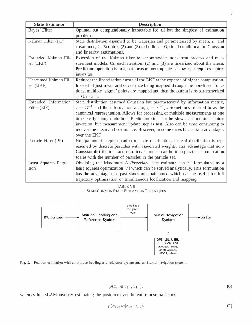
Often state estimation is decomposed into two parts: attitude heading and reference system (AHRS) and inertialnavigation system (INS) as shown in Fig. 2 . All sensors that give information about Euler angles or rates areinputs into the AHRS, which produces a stable estimate of vehicle orientation. The stabilized roll, pitch, and yaware then used by the INS in combination with other sensors that give information about vehicle position, linearvelocity, or linear acceleration to estimate the vehicle position.

C. Simultaneous Localization and Mapping

Simultaneous localization and mapping (SLAM) is the process of a robot autonomously building a map of itsenvironment and, at the same time, localizing itself withinthat environment1. SLAM algorithms can be eitheronline, where only the current pose is estimated along with the map,or full where the posterior is calculated overthe entire robot trajectory [6] . Analytically, online SLAMinvolves estimating the posterior over the momentarypose,xt, and the map,m given all measurements,z1:t, and inputsu1:t

1also referred to as concurrent mapping and localization

6

State Estimator DescriptionBayes’ Filter Optimal but computationally intractable for all but the simplest of estimation

problems.Kalman Filter (KF) State distribution assumed to be Gaussian and parameterized by mean,µ, and

covariance,Σ. Requires (2) and (3) to be linear. Optimal conditional on Gaussianand linearity assumptions.

Extended Kalman Fil-ter (EKF)

Extension of the Kalman filter to accommodate non-linear process and mea-surement models. On each iteration, (2) and (3) are linearized about the mean.Prediction operation is fast, but measurement update is slow as it requires matrixinversion.

Unscented Kalman Fil-ter (UKF)

Reduces the linearization errors of the EKF at the expense ofhigher computation.Instead of just mean and covariance being mapped through thenon-linear func-tions, multiple ‘sigma’ points are mapped and then the output is re-parameterizedas Gaussian.

Extended InformationFilter (EIF)

State distribution assumed Gaussian but parameterized by information matrix,I = Σ−1 and the information vector,ζ = Σ−1µ. Sometimes referred to as thecanonical representation. Allows for processing of multiple measurements at onetime easily though addition. Prediction step can be slow as it requires matrixinversion, but measurement update step is fast. Also can be time consuming torecover the mean and covariance. However, in some cases has certain advantagesover the EKF.

Particle Filter (PF) Non-parametric representation of state distribution. Instead distribution is rep-resented by discrete particles with associated weights. Has advantage that non-Gaussian distributions and non-linear models can be incorporated. Computationscales with the number of particles in the particle set.

Least Squares Regres-sion

Obtaining the MaximumA Posteriori state estimate can be formulated as aleast squares optimization [7] which can be solved analytically. This formulationhas the advantage that past states are maintained which can be useful for fulltrajectory optimization or simultaneous localization andmapping.

TABLE VIISOME COMMON STATE ESTIMATION TECHNIQUES

Attitude Heading and

Reference System

Inertial Navigation

SystemIMU, compass

GPS, LBL, USBL,

SBL, SLAM, DVL,

acoustic range,

depth sensor,

ADCP, others

stabilized

roll, pitch,

yaw

position

Fig. 2. Position estimation with an attitude heading and reference system and an inertial navigation system.

p(xt,m|z1:t, u1:t), (6)

whereas full SLAM involves estimating the posterior over the entire pose trajectory

p(x1:t,m|z1:t, u1:t). (7)

7

L1

L2

L3

L4

L5

L8

L6

L7

L9

V1 V2

V3

V4

P1P2

P3

P4

P1P2

P3

P4

a) b)

Fig. 3. (a) Feature based SLAM, (b) View based SLAM.

In addition, SLAM implementations can be classified asfeature based, where features are extracted (detection,identification and classification) and maintained in the state space, orview based, where poses corresponding tomeasurements are maintained in the state space.

As Fig. 3-a shows, in feature based SLAM features are extracted from sensor measurements. For example, at poseP1 the robot sees three featuresL1, L2 andL3. These features together with the pose of the robot are maintainedin the state space. At the next pose,P2, only newly observed features,L4 andL5 are added to the vector and thepose is replaced with the previous pose. This process occursat each new pose. In view based SLAM (Fig. 3-b), ateach pose the whole view without extracting any features is processed usually by comparing it with the previousview. For example, at poseP3, V3 is compared withV2 to find the view based odometry. State vectors in this casecan be composed by one or more of the poses at each time.

SLAM method Pros Cons AUVApplication

EKF SLAM [14] Works well when features arepresent and distinct (which can bechallenging underwater ).

Adding new features to state spacerequires quadratic time.

[15] [16] [17][18] [19] [20][21] [22]

SEIF SLAM [23] Performs updates in constant time.Due to additivity of information, itis a good choice for multiple-robotSLAM.

Information matrix has to be ac-tively ‘sparsified’. Recovering maprequires matrix inversion.

[24] [25] [26]

FastSLAM [27] Logarithmic time in numberof features. No dependance onparametrization of motion models.

Ability to close loops depends onparticle set.

[28] [29] [30][31] [32]

GraphSLAM [33] Previous poses are updated forpost-processing of data.

More computation required. Co-variances are hard to recover (in-formation form).

[34] [35]

AI SLAM Efficient, because it mimics theway animals brain work.

Requires training or parameter tun-ing.

[36]

TABLE VIIISTRENGTHS AND WEAKNESSES OFSOME COMMON SLAM TECHNIQUES

Filtering (online) approaches to SLAM make use of a state estimation algorithm such as those presented in TableVII. Smoothing (full SLAM) methods, also known as GraphSLAM[33], minimize the process and observationconstraints over the whole trajectory of the robot. Some approaches use a combination of methods.

Some of the most popular categories of SLAM approaches are described here with their pros, cons, and AUV

8

navigation references provided in Table VIII. The categorization is based on [6] with some additions:

• EKF SLAM : EKF-SLAM linearizes the system model using the Taylor expansion. It applies recursive predict-update cycle to estimate pose and map. Its state vector includes pose and features [14]. It is applicable toboth view based SLAM [37] and feature based SLAM [38]. For large maps, EKF-SLAM is computationallyexpensive since computation time scalesO(n2) wheren is the number of features.

• SEIF SLAM : Sparse extended information filter (SEIF) [23] and exactlysparse extended information filters(ESEIF) [39] are two well-known approaches for SLAM using the information filter. They both maintain asparse information matrix which preserves the consistencyof the Gaussian distribution; however, accessingthe mean and covariance requires a computationally expensive large matrix inversion. Both approaches needthe information matrix to be actively ‘sparsified’ by a sparsification strategy. ESEIF maintains an informationmatrix with the majority of elements beingexactlyzero which avoids the overconfidence problem of [23].

• FastSLAM: FastSLAM is based on the particle filter. Particle filteringapproaches are nonlinear filteringsolutions; therefore, the system models are not approximated. In FastSLAM, poses and features are representedby particles (points) in the state space [27]. FastSLAM is the only solution which performs online SLAMand full SLAM together, which means it estimates not only thecurrent pose, but also the full trajectory. InFastSLAM, each particle holds an estimate of the pose and allfeatures; however, each feature is representedand updated through a separate EKF. Similar to other methods, it is applicable to both view based SLAM [40]and feature based SLAM [6].

• GraphSLAM : In GraphSLAM methods, the entire trajectory and map are estimated [33]. GraphSLAM alsouses approximation by Taylor expansion, however it differsfrom EKF-SLAM in that it accumulates informationand therefore is considered to be an off-line algorithm [6].Generally, in GraphSLAM, poses of the robotare represented as nodes in a graph. The edges connecting nodes are modeled with motion and observationconstraints. These constraints need to be optimized to calculate the spatial distribution of the nodes andtheir uncertainties [6]. Different solutions exist for GrpahSLAM such as relaxation on a mesh [41], multi-levelrelaxation [42], iterative alignment [43], square root smoothing and mapping (SAM) [7], incremental smoothingand mapping (iSAM) [44] and works by Grisetti et. al in [45], [46], and hierarchical optimization for posegraphs on manifolds (HOGMAN) [47]. In principle, they are all similar, but differ in how the optimizationis implemented. For instance, iSAM solves the full SLAM problem by updating a matrix factorization whileHOGMAN’s optimization is performed over a manifold.

• Artificial Intelligence (AI) SLAM : These methods of SLAM are based on fuzzy logic and neural networks.ratSLAM [48] is a technique that models rodents’ brain usingneural networks. In fact this method is neuralnetwork-based data fusion using a camera and an odometer. [49] uses self organizing maps (SOM) to performSLAM with multiple-robots. The SOM is a neural network whichis trained without supervision.

The choice of the method for estimating the poses of robots and the map depends on many factors such as theavailable memory, processing capability and type of sensory information.

SLAM techniques have been used for acoustic (Sec. IV) and particularly geophysical (Sec. V) underwaternavigation algorithms as will be described.

D. Cooperative Navigation

In cooperative navigation (CN), AUV teams localize using proprioceptive sensors as well as communicationsupdates from other team members.

CN finds its origin in ground robotics applications. In the seminal paper by Roumeliotis and Bekey [50], itis proven that a group of autonomous agents with no access to global positioning can localize themselves moreaccurately if they can share pose estimates and uncertaintyas well as make relative measurements. In [51], thescalability of CN is addressed, and it is shown that an upper bound on the rate of increase of position uncertaintyis a function of the size of the robot team. Other important results have been proven, such as that the maximumexpected rate of uncertainty increase is independent of theaccuracy and number of inter-vehicle measurementsand depends only on the accuracy of the proprioceptive sensors on the robots [52]. In addition, applications ofMaximum A Posteriori [53], [54], EKF [55] and nonlinear least squares [56] estimators have been developed forgeneral robotics CN. A complexity analysis is also presented in [57]. Special considerations must be made to apply

9

x1, y1, z1

x2, y2, z2

x3, y3, z3

R23,R32

R12,R21

R13,R31

σy3,y3

σx3,x3

σy1,y1

σx1,x1

σy2,y2

σx2,x2

Actual Position

Estimated Position

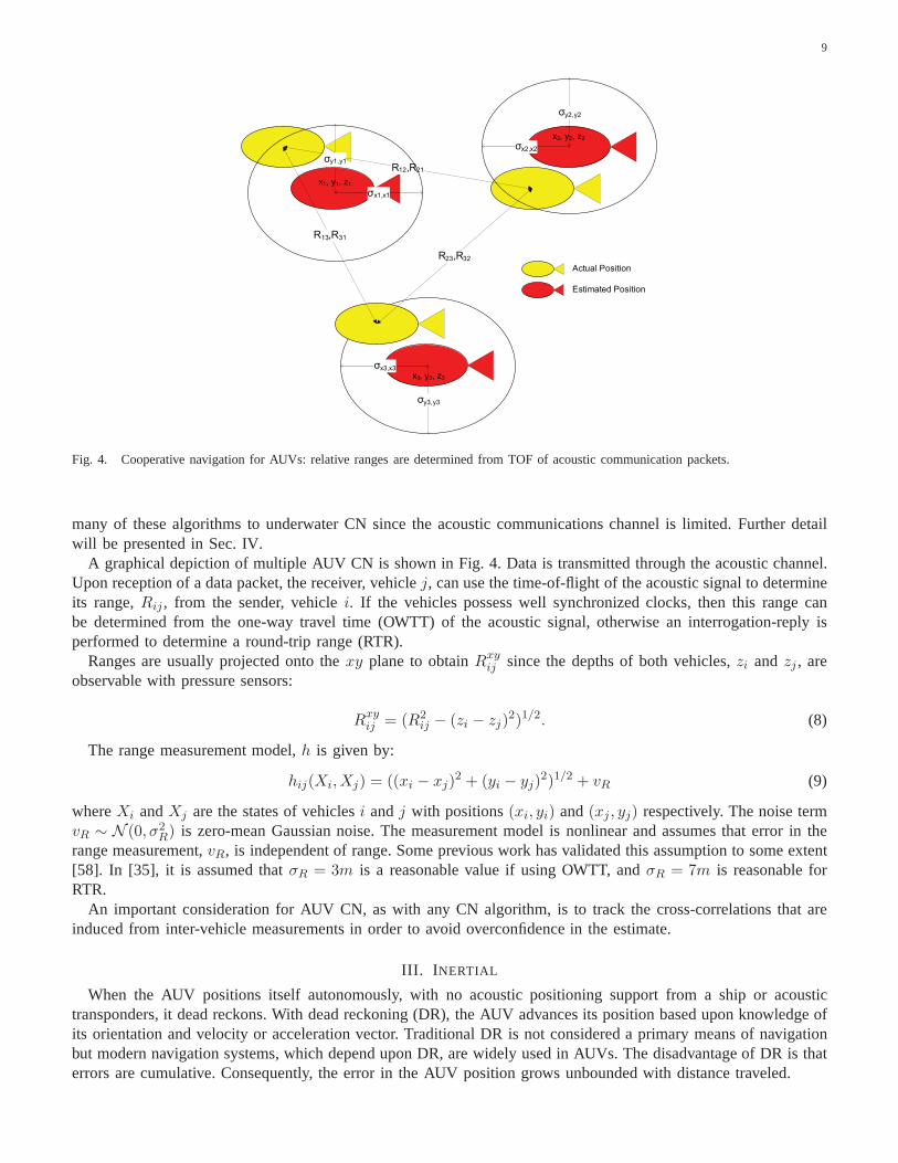
Fig. 4. Cooperative navigation for AUVs: relative ranges are determined from TOF of acoustic communication packets.

many of these algorithms to underwater CN since the acousticcommunications channel is limited. Further detailwill be presented in Sec. IV.

A graphical depiction of multiple AUV CN is shown in Fig. 4. Data is transmitted through the acoustic channel.Upon reception of a data packet, the receiver, vehiclej, can use the time-of-flight of the acoustic signal to determineits range,Rij , from the sender, vehiclei. If the vehicles possess well synchronized clocks, then this range canbe determined from the one-way travel time (OWTT) of the acoustic signal, otherwise an interrogation-reply isperformed to determine a round-trip range (RTR).

Ranges are usually projected onto thexy plane to obtainRxyij since the depths of both vehicles,zi and zj , are

observable with pressure sensors:

Rxyij = (R2

ij − (zi − zj)2)1/2. (8)

The range measurement model,h is given by:

hij(Xi,Xj) = ((xi − xj)2 + (yi − yj)

2)1/2 + vR (9)

whereXi andXj are the states of vehiclesi andj with positions(xi, yi) and(xj , yj) respectively. The noise termvR ∼ N (0, σ2R) is zero-mean Gaussian noise. The measurement model is nonlinear and assumes that error in therange measurement,vR, is independent of range. Some previous work has validated this assumption to some extent[58]. In [35], it is assumed thatσR = 3m is a reasonable value if using OWTT, andσR = 7m is reasonable forRTR.

An important consideration for AUV CN, as with any CN algorithm, is to track the cross-correlations that areinduced from inter-vehicle measurements in order to avoid overconfidence in the estimate.

III. I NERTIAL

When the AUV positions itself autonomously, with no acoustic positioning support from a ship or acoustictransponders, it dead reckons. With dead reckoning (DR), the AUV advances its position based upon knowledge ofits orientation and velocity or acceleration vector. Traditional DR is not considered a primary means of navigationbut modern navigation systems, which depend upon DR, are widely used in AUVs. The disadvantage of DR is thaterrors are cumulative. Consequently, the error in the AUV position grows unbounded with distance traveled.

10

One simple method of DR pose estimation, for example if heading is available from a compass and velocity isavailable from a DVL , is achieved by using the following kinematic equations:

x = v cosψ + w sinψ

y = v sinψ + w cosψ

ψ = 0

(10)

where(x, y, ψ) is the displacement and heading in the standard North-East-Down coordinate system, andv, andware the body frame forward and starboard velocities. In thismodel it is assumed that roll and pitch are zero andthat depth is measured accurately with a depth sensor.

An inertial system aims to improve upon the DR pose estimation by integrating measurements from accelerometersand gyroscopes. Inertial proprioceptive sensors are able to provide measurements at a much higher frequency thanacoustic sensors that are based on the TOF of acoustic signals. As a result, these sensors can reduce the growthrate of pose estimation error, although it will still grow without bound.

One problem with inertial sensors is that they drift over time. One common approach, for example used in [11],is to maintain the drift as part of the state space. Slower rate sensors are then effectively used to calibrate theinertial sensors. In [11], the authors also track other possible sources of error such as the variable speed of soundin water to reduce systematic noise. These noise sources arepropagated using a random walk model, and thenupdated from DVL or LBL sensor inputs. Their INS is implemented with an IMU that runs at 150Hz.

The basic kinematics model (10) is incomplete if the local water current is not accounted for. The current canbe measured with an acoustic Doppler current profiler (ADCP). For implementations with ADCP see [9] [10]. ADVL is usually able to calculate the velocity of the water relative to the AUV,vb and the velocity of the seabedrelative to the AUV,vg. Then the ocean current can be calculated easily asvc = vg - vb . The ocean current canalso be obtained from an ocean model, for example in [59] where ocean currents are predicted using the regionalocean modeling system [60] combined with a Gaussian processregression [61]. If access to the velocity over theseabed is not available, then the current can be estimated from a transponder on a surface buoy as in [62]. In [62],the authors analyzed the power spectral density to remove the low frequency excitation on the buoy due to thewaves to estimate the underwater current.

In [8], an algorithm based on particle filtering is proposed that exploits known bathymetric maps - if they exist.It is emphasized that the tide level must be carefully monitored to avoid position errors, particularly in areas oflow bathymetric variation. This approach is referred to as “terrain-aided navigation”, and the method is comparedfor DVL, and multi-beam sonars as the bathymetric data input, concluding that both are viable options.

The performance of an INS is largely determined by the quality of its inertial measurement units. In general, themore expensive the unit, the better its performance. However, the type of state estimation also has an effect. Themost common filtering scheme is the EKF, but others have been used to account for the linearization and Gaussianassumption shortcomings of the EKF. For example, in [63] a UKF is used and in [64] a PF application is presented.

Improvements can also be made to INS navigation by modifyingEq. (10) to provide a more accurate model ofthe vehicle dynamics. The benefits of such an approach are investigated in [65], particularly in the case that DVLloses bottom lock, for example.

Inertial sensors are the basis of an accurate navigation scheme, and have been combined with other techniquesdescribed in subsequent sections. In certain applications, navigation by inertial sensors is the only option. Forexample, in extreme depths where it is impractical to surface for GPS, an INS is used predominantly, as describedin [66].

The best INS can achieve a drift of 0.1% of the distance traveled [35], however, more typical and modestlypriced units can easily achieve a drift of 2-5% of the distance traveled.

IV. A COUSTIC TRANSPONDERS ANDBEACONS

In acoustic navigation techniques, localization is achieved by measuring ranges from the TOF of acoustic signals.Common methods include:

• Ultra Short Baseline (USBL): Also sometimes called super short baseline (SSBL). The transducers on thetransceiver are closely spaced with the approximated baseline on the order of less than10 centimeters. Relative

11

Fig. 5. (a) Short Baseline (SBL) (b) Ultra-Short Baseline (USBL) (c) Long Baseline (LBL)

ranges are calculated based on the TOF and the bearing is calculated based on the difference of the phase ofthe signal arriving at the transceivers. See Fig. 5-b.

• Short Baseline(SBL): Beacons are placed at opposite ends of a ship’s hull. The baseline is based on the sizeof the support ship. See Fig. 5-a.

• Long Baseline (LBL) and GPS intelligent Buoys (GIBs): Beacons placed over a wide mission area.Localization is based on triangulation of acoustic signals. See Fig. 5-c. In the case of GIBs, the beaconsare at the surface whereas for LBL they are installed on the seabed.

• Single Fixed Beacon: Localization is performed from only one fixed beacon.• Acoustic Modem: The recent advances with acoustic modems have allowed for new techniques to be devel-

oped. Beacons no longer have to be stationary, and full AUV autonomy can be achieved with support fromautonomous surface vehicles, equipped with acoustic modems, or by communicating and ranging in underwaterteams.

Due to the latency of acoustic updates, state estimators areimplemented where the dead reckoning proprioceptivesensors provide the predictions and then acoustic measurements provide the updates.

A. Ultra Short and Short Baseline

Ultra short baseline (USBL) navigation allows an AUV to localize itself relative to a surface ship. Relative rangeand bearing are determined by TOF and phase differencing across an array of transceivers, respectively. A typicalsetup would be to have a ship supporting an AUV. In short baseline (SBL), transceivers are placed at either end ofthe ship hull and triangulation is used.

The major limitation of USBL is the range and of SBL is that thepositional accuracy is dependent on the sizeof the baseline, i.e. the length of the ship.

In [67] an AUV was developed to accurately map and inspect a hydro dam. A buoy equipped with an USBL anddifferential GPS helps to improve upon dead reckoning of theAUV which is performed using a motion referenceunit (MRU), a fibre optic gyro (FOG) and a DVL. An EKF is used to fuse the data and a mechanical scanningimaging sonar (MSIS) tracks the dam wall and follows it usinganother EKF. For this application, the USBL isa good choice because the range required for the mission is small. The method proposed in [12] augments [67]by using a delayed-state information filter to account for the time delay in the transmission of the surface shipposition.

In [68], sensor based integrated guidance and control is proposed using a USBL positioning system. The USBLis installed on the nose of the AUV while there is an acoustic transponder installed on a known and fixed positionas a target. While homing, the USBL sensor listens for the transponder and calculates its range and the bearingbased on the time difference of arrival (TDOA). In [69], USBLis used for homing during the recovery of an AUVthrough sea ice.

In [70], two methods are presented to calibrate inertial andDVL sensors. The inertial navigation system datafrom the AUV is sent to the surface vehicle by acoustic means.In one method a simple KF implementation is usedwhich maintains the inertial sensor drift errors in the state space. In the other method, possible errors of the USBLin the sound velocity profile are incorporated and the EKF is used to fuse data. No real hardware implementation isperformed. In [71], the method is extended to multiple AUVs by using an “inverted” setup where the the transceiveris mounted on the AUV and the transponder mounted on the surface ship.

12

In [72], data from an USBL and an acoustic modem is fused by a particle filter to improve dead reckoning.As a result, the vehicle operates submerged longer as GPS fixes can be less frequent. The simulation and fieldexperiments verify the developed technique.

In [73], a ‘tightly-coupled’ approach is used where the spatial information of the acoustic array is exploited tocorrect the errors in the INS.

B. Long Baseline / GPS Intelligent Buoys

In LBL navigation, localization is achieved by triangulating acoustically determined ranges from widely spacedfixed beacons. In most cases, the beacons are globally referenced before the start of the mission by a surface ship[74], a helicopter [75], or even another AUV [76]. In normal operation, an AUV would send out an interrogationsignal, and the beacons would reply in a predefined sequence.The two way travel time (TWTT) of the acousticsignals is used to determine the ranges. However, there havebeen implementations in which synchronized clocksare used to support one-way travel time (OWTT) ranging [77].

GIBs remove the need for the LBL beacons to be installed at theseafloor which can reduce installation costsand the need for recovery of these beacons.

One of the limitations of LBL is the cost and time associated with setting up the network. However, this canbe mitigated to some extent if the beacon locations are not globally referenced and either self-localize [78], or theAUV can localize them by performing SLAM. For example, [34] uses a nonlinear least squares implementation,whereas [79] uses a particle filter version of SLAM to determine the location of the fixed beacons during themission.

A major consideration in an LBL localization network is the treatment of outliers. Methods to account for outliersin LBL systems include hypothesis grids [80] and graph partitioning [81]. Generally, range measurements can fallinto one of three categories: direct path (DP), multi-path (MP), or outlier (OL). From experience, range errorsare not Gaussian distributions. The quality of range data isdependent on the location within the survey area. In[80], a hypothesis grid is built to represent the belief thatfuture measurements from a particular cell will be ina particular category (i.e. DP, MP, OL). In graph partitioning, outliers are rejected using spectral analysis. A setof measurements is represented as a graph, then the graph partitioning algorithm is applied to identify sets ofconsistent measurement [81].

Another consideration is the TDOA of the acoustic responsesof the network [82], [83]. The change in vehiclepose between the initial interrogation request and all of the subsequent replies must be explicitly handled. This isoften done with a delayed state EKF.

Each range difference measurement between two receivers constrains the target to a annulus (in 2D) or a sphere(in 3D). Annuluses are intersected to find the location of thetarget. However, when the data is corrupted bynoise, there is not necessarily an intersection point. Sequential quadratic programming [84] is used to perform theconstrained optimization. The target position estimate isthe same as the traditional maximum likelihood estimate.

Major drawbacks of LBL are the finite range imposed by the range of the beacons, and the reliance on preciseknowledge of the local sound velocity profile of the water column based on temperature, salinity, conductivity,and other factors [74]. However, the LBL systems do overcomethese shortcomings to be one of the most robust,reliable, and accurate localization techniques available. For that reason it is often used in high-risk situations suchas under-ice surveys [75], [85]. Other implementations include: alignment of Doppler sensors [86] and deep watersurveys [87]. An extensive evaluation of the precision of LBL is provided in [88].

As a surveying implementation example, in [87] a technique is used for deep sea near bottom survey by an AUVwhich relies on LBL for navigation. LBL transponders are GPS-referenced before the start of the survey.

In [86], two techniques forin situ 3 degrees-of-freedom calibration of attitude and Doppler sonar sensors areproposed. LBL and gyrocompass measurements are sources of information for alignment.

C. Single Fixed Beacon

A downside of LBL systems is the cost and time required for installing the beacons and geo-referencing them. Itis possible to reduce these infrastructure requirements ifonly a single fixed beacon is used instead of a network ofthem. The concept is that the baseline is simulated by propagating the ranges from a single beacon forward in timeuntil the next update is received. This technique has been referred to as virtual LBL (VLBL) and has been simulated

13

Fig. 6. An AUV localizing with a single fixed beacon at known location. Uncertainty grows in between updates from the beacon. Onreception of an update from the beacon, uncertainty is reduced in the dimension coinciding with the location of the beacon.

on real world data in [89]. It is noted that the AUV trajectoryhas a significant effect on the observability of thevehicle state. Long tracks directly towards or away from thesingle fixed beacon will cause unbounded growth inposition error. As a result, tracks or paths for the survey vehicle being localized in this manner should be plannedto be tangential to range circles emanating from the transponder.

A visual representation of single beacon navigation is shown in Fig. 6. It assumes that the vehicle has priorknowledge of the beacon location. In the figure the vehicle receives 3 acoustic pings from the beacon at thebottom. Each time, reception of a ping results in a reductionof uncertainty in the direction of the beacon.

An important consideration when the baseline is removed is observability of the state space. As detailed in [90],and elaborated upon in [91] and [92], if the states are estimated by a linearized filter, such as an EKF or EIF,then observability is lost if repeated range updates come from the same relative bearing. However, if the statesare estimated with a nonlinear filter, then the condition forloss of observability changes to repeated range updatescoming from the same relative bearing and the same range. As aresult of the nonlinear nature of the range updatemodel, it is beneficial to use a nonlinear state estimator from an observability standpoint. This is derived in detailin [91] and [92] using Lie derivatives to generate the observability matrix.

Single beacon navigation has also been used for homing, for example in [93]. This task is particularly challengingbecause the AUV will preferentially move in a track directlytowards the beacon, violating the observability criterion.As a result, path planning must be designed to avoid this situation. This can be particularly useful for recoveringan AUV that has become inoperable, but is still able to transmit pings.

D. Acoustic Modem

Advances in the field of acoustic communications have had a major effect on underwater navigation capabilities.The acoustic modem allows simultaneous communication of small packets and ranging based on TOF. If theposition of the transmitter is included in the communicatedinformation, then the receiver can bound its position toa sphere centered on the transmitter. This capability removes the need for beacons to be fixed or localized prior tothe mission. In addition, it allows for inter-AUV communication, which means teams of AUVs can cooperativelylocalize.

Popular acoustic modem are manufactured by Woods Hole Oceanographic Institute [94], Teledyne Benthos [95],and Evologics [96] among others . In general communication can either use frequency shift keying with frequencyhopping (FH-FSK), which is more reliable but provides lowerdata rates, or variable rate phase-coherent keying(PSK). Some models also include precise pulse-per-second (PPS) clocks (eg [97]) to allow synchronous ranging.Typically, due to the limited bandwidth underwater, the communication channel is shared using a time-divisionmultiple access (TDMA) scheme. In TDMA, each member in the group is allotted a time slot with which tobroadcast information. The major detractor of such a schemeis that the total cycle time grows with group size. Atpresent, achievable bit rates range from 32 bytes per 10s packet with FSK, to several kbit/s in optimal conditionswith PSK.

1) Manned Surface Support:The ability of a modem at the surface to transmit its locationto the survey vehiclesprovides two important benefits over past navigation methods: 1) it removes the necessity to geo-reference the

14

beacons prior to starting the mission, and 2) It allows the beacons to move during the missions. The first advantagesaves time and money, and the second allows the mission rangeto be extended as necessary without re-deployingthe sensor network. Many methods have been recently published that exploit one or both of these benefits.

The moving long baseline (MLBL) concept was first demonstrated in [98] using a Sonardyne AvTrack acousticnavigation system. Two manned surface vehicles were used tosupport one AUV. This concept has proved particularlyuseful for mapping rivers, such as [99]. In this project, twoboats are used to continuously define a cross-sectionof the river to be mapped near the location of the AUV.

This approach has been extended to a single moving source. A manned surface ship can localize itself withGPS and bound the error of one or more survey AUVs by broadcasting its position. Such an approach is attractivebecause there is no need for calibration or recovery of beacons. The approach is similar to that presented in Sec.IV-C except the mission range can be much larger because the surface vehicle can move.

In [100] and [13], a deep water validation was performed for the single moving beacon concept. It should benoted that localization is done in post-processing. In the proposed approach, an EKF maintains an estimate of thesurvey vehicle as well as the support ship. In a deep water application, the time taken for the acoustic transmissionshould be accounted for in the filtering algorithm. Here, this is represented as a delayed state EKF. It is accuratelynoted that the TOF measured is the range between the current position of the receiver and a previous position ofthe sender. In [13], the performance of the single beacon navigation is compared against an LBL system. Also,there is a more rigorous discussion on sources of error in acoustic range measurements such as errors in soundvelocity estimation, acoustic multi-path, and errors in ship GPS. Similarly, in [101] a deep diving AUV is localizedin post-processing. In this case, the survey vehicle is required to execute a known closed path after it dives to adepth of 6000m. A similar approach is presented in [102] to map the magnetic signature of a moving vessel.

If the survey vehicles are acting as passive listeners usingOWTT for range measurement, then the systemnaturally scales well with number of survey vehicles assuming they stay within range of the surface vehicle. In[103] and [104], a maximum likelihood sensor fusion technique is presented to localize survey vehicles to within1m over a 100km survey. It is also noted in this paper that overa long survey, the drift of the PPS clock will havea significant effect on the localization performance.

2) Autonomous Surface Crafts:Once it is established that AUVs can navigate with the help ofmanned surfacevehicles, a natural progression to increase autonomy is to move towards unmanned surface vehicles. The firstknown implementation of autonomous surface crafts (ASCs) used to support AUVs is presented in [58], which isan extension of the MLBL concept presented in [98]. Two ASCs are used to support one Odyssey III AUV in aseries of experiments in 2004 and 2005. In [105], two ASCs areused and a general framework is developed forcooperative navigation.

Following previous trends, the logical progression was to perform AUV navigation and localization with onlyone ASC. This has been experimentally shown in [91] and [106]. The approaches taken were similar, but in [106],no actual AUVs were used in the implementation, instead an ASC was used as a surrogate. In both cases, theauthors implemented a nonlinear least squares (NLS) approach. In [91], the experimental validation is done usingan ASC and an AUV to compare the performance of the EKF, PF, andan NLS optimization. It is shown that theNLS performs the best, particularly after off-line post-processing. The observability is carefully considered in bothcases. In [91], it is shown that the observability criterionis less stringent if the states are being estimated witha nonlinear filter. In addition, the ASCs autonomy includes basic heuristics for supporting the survey AUV andmaintaining observability by performing different motionbehaviors. In addition, in [91], an error analysis of therange updates is performed, and the noise found to be relatively close to normally distributed and independent ofrange.

Path planning of the ASC to maintain observability is also considered explicitly in [107]. More recently, anobservability analysis was done for an ASC/AUV team under the cases that position, and that position and velocity,are transmitted from the ASC to the AUV [108]. A method for globally asymptotically stable observer design isalso presented. In [109], an AUV is able to localize relativeto a surface ship or a drifter whose position is estimatedwith the use of an ocean current model. Furthermore, the AUV is able to obtain relative range and bearing estimatesby detecting the surface ship or buoy using an upward-looking sonar. A theoretical analysis of the benefits of suchan approach as well as performance bounds are derived.

It is expected that in the coming years, ASCs, such as the waveglider [110], will be capable of providingextremely long-term autonomous navigation capabilities.One such example scenario is presented in [111] where a

15

wave glider is used to localize an active acoustic source.3) Heterogeneous AUV Teams:In some cases, certain AUVs are outfitted with more expensivesensors and/or

make frequent trips to surface for GPS position fixes. These vehicles support the other survey vehicles and havebeen referred to as communications/navigations aids (CNAs)2. An application would be to have inferior navigationsensors on a fleet of survey vehicles and expensive navigation sensors on only a small number of vehicle whosejob is to support that fleet [112]. Upon reception of a CNA transmission the receiver’s position estimate can berestricted to an annulus if each vehicle has a good estimate of depth (which can easily be obtained from a pressuresensor), and if the receiver can estimate its range to the CNA, for example through either one-way TOF of theacoustic signal (requires synchronized clocks) or two-wayTOF . This annulus can be intersected with a vehicle’sown covariance ellipse as shown in Fig. 7.

`

Fig. 7. A CNA AUV supporting a survey AUV [112]. The blue areasare the vehicle uncertainty ellipses. The yellow area is theupdateduncertainty of the survey ellipse from a range measurement,which is shown in pink.

The framework for cooperative navigation developed by Bahrand others is presented in [113], [105], [114],[115] and is applicable to general AUV teams. Referring to Fig. 7, each annulus is propagated forward in timeuntil the next update is received from the CNA. In between updates, the uncertainty grows based on the quality ofthe DR estimation. The importance of careful book-keeping and maintenance of cross-correlations between surveyand CNA AUVs is stressed to avoid over-confidence and to enhance the quality of outlier rejection. While thedeveloped framework is to be used for pure AUV systems, all results show the use of ASCs as “surrogate AUVs”.

An altogether different approach to CN is presented in [116]where a hovering type AUV can physically dockto the torpedo type AUV in order to exchange information.

4) Homogeneous AUV Teams:When a homogeneous team performs CN, each member of the team is treatedequally. Position error will grow slower if the AUVs are ableto communicate their relative positions and ranges.Similarly to the heterogeneous case, if any vehicle surfaces for a position fix, then the information can be sharedwith the rest of the team to bound the position error.

The first known experimental implementation of such a systemwas in 2007 [117]. In this approach, the vehiclestates are maintained with an EKF but cross covariances are not transmitted in the communications packet due tobandwidth limitations. The communication latency is accounted for in the EKF implementation.

More recently, an implementation of CN was presented in [118]. Here, the issue of book-keeping is explicitlyaddressed. A multi-vehicle ledger system is used so updatesare only made to the multi-vehicle EKF when all upto date data has been obtained. Experiments were performed with kayaks acting as AUV surrogates, where OWTTranging was done with the synchronized clocks in a 30s cycle,each of the three vehicles having a 10s slot to makea transmission.

V. GEOPHYSICAL

Geophysical navigation refers to any method that utilizes external environmental features for localization. Almostall methods in this category that achieve bounded position error use some form of SLAM. Categories include:

2This term has also been applied to surface vehicles supporting AUV survey teams

16

• Magnetic: It has been proposed to use magnetic field maps for localization. Although no recent publicationshave been found, a team at the University of Idaho has been mapping the magnetic signatures of Navy vessels[119], [120].

• Optical: Use of a monocular or stereo camera to capture images of the seabed and then match these imagesto navigate.

• Sonar: Used to acoustically detect then identify and classify features in the environment that could be usedas navigation landmarks. With bathymetric sonar features can be extracted almost directly from assembledreturns. With sidescan (imaging) sonar, feature extraction is achieved through processing of imagery.

A. Optical

Visual odometry is the process of determining the robot poseby analyzing subsequent camera images. Thiscan be achieved through optical flow or structure from motion(SFM). Invariant extraction and representation offeatures is an important consideration. Many previous algorithms have been proposed and applied in ground and airrobotics, such as scale-invariant feature transform (SIFT) [121], speeded up robust feature (SURF) [122], amongstmany others3. Images can be captured with either stereo or monocular cameras. Stereo cameras have the addedadvantage that full 6 degree-of-freedom transformations between consecutive image pairs can be found. Vision-based SLAM can also be performed with the methods presented in Table VIII. The major challenge is closing loopsin the trajectory by associating non-consecutive images, which is necessary to bound localization error.

Limitations for optical systems in underwater environments include the reduced range of cameras, susceptibilityto scattering, and inadequacy of lighting. As a result, visible wavelength cameras are more commonly installed onhovering AUVs because they can get close to objects of interest. In addition, visual odometry and feature extractionrelies on the existence of features. Therefore optical underwater navigation methods are particularly well-suited tosmall-scale mapping of feature-rich environments. Examples include ship hulls or shipwreck inspections.

In [16] and [17], Eustice et al. present an implementation ofunderwater vision-based SLAM called visuallyaugmented navigation (VAN). The multi-sensor approach combines the benefits of optical and inertial navigationmethods and is robust to low overlap of imagery. The approachis a view based version of EKF-SLAM, wherecamera-derived relative pose measurements provide the spatial constraints for visual odometry and loop closure. In[24] and [25], the VAN approach is converted to the information form and it is proven that the view based ESEIFSLAM maintains a sparse information matrix without approximations or pruning. This approach was applied todeep water surveying of the RMS Titanic in [24] . The issue of recovering the mean and the covariance from theinformation form is also addressed. SIFT and Harris extraction points are used to match images. The VAN methodhas also been applied to ship-hull inspection for the US Navy[124]. Both [44] and [125] were inspired by theVAN method. However, these two methods improved upon the approach using a smoothing and mapping problemformulation and doing efficient matrix factorizations to beable to efficiently recover the means and covariances. Inrecent work, [126] uses features from both a profiling sonar and a monocular camera in full pose graph formulationfor a hovering AUV performing ship hull inspections. Odometry is derived relative to the ship hull using a DVLlocked onto the ship. An approach to tackle the problem of data association in feature-poor areas of a ship hull isexplored in [127] using a novel online bag-of-words approach to determine inter-image and intra-image saliency.

Feature based approaches to underwater SLAM have also been done. For example, in [18], an augmented EKFis used to generate a topological representation. Non-time-consecutive images are compared and loop closuresare made based on observation mutual information. Feature based EKF SLAM is also applied to the underwaterenvironment in [19] and [20].

A byproduct of accurate localization is that accurate mapping can be achieved. Several authors have shown theability to compute 2D and 3D reconstructions of the underwater environment based on optical underwater SLAM.For example, in [128], an SFM model together with SLAM are used to photomosaic the RMS Titanic as well asa hydrothermal vent area in the mid-Atlantic. In [129], 3D reconstructions of an underwater environment are doneusing SLAM with a combination of multi-beam sonar and stereocamera.

Future research will likely involve incorporating multiple vehicles. Recently, some publications involving simu-lations report on this [130], [131]. Overcoming communications constraints will be a major challenge.

3For a review and comparison of some methods, see [123].

17

Pure visual odometry based methods that do not require SLAM can be used for applications such as pipelinetracking [132].

B. Sonar

Sonar imaging of the ocean pre-dates AUVs by decades. As a result, it is a fairly robust technology. Severaltypes of sonars are used for seabed and structure mapping. They can be categorized as imaging-type which providean image of the seabed (see Table IV) and ranging-type which produce range or bathymetric data (see Table X).

Sonar Description Pros Trade-Off ApplicationSidescan multiple beams that measure

intensity of returns to create a2D image of sea bed; beamsare directed perpendicular totravel direction.

can work at rela-tively high speeds(10kt) to give higharea coverage.

resolutioninverselyproportionalto range, e.g. 1.8MHz produces40 m range.

[133] [35] [134][135]

ForwardLook(imagingtype)

similar in principle to a side-scan sonar only beams are di-rected forward.

obstacle avoidance,also as a nadir gapfiller.

limited distance todepth ratio ( 6:1max); single angleof view.

[26] [136]

SyntheticAperture

coherent processing of con-secutive displaced returns tosynthesize a virtual array.

range independentresolution

optimal at lowspeeds and deeperwater.

[137] [138][139]

MechanicalScannedImagingSonar

One beam with actuator thatscans a swath.

Cheaper than multi-beam.

Slow. Accuracydepends on AUVattitude.

[15], [21],[140], [141],[142], [143],[22]

TABLE IXIMAGING-TYPE SONAR DEVICES USED FORUNDERWATERNAVIGATION

Sonar Description Pros Trade-Off ApplicationEchoSounder

single, narrow beamused to determinedepth below thetransducer.

yield representation ofsea bed and targetsbetween transducer toseabed.

point measurements in gen-erally one direction.

[144],[145]

Profiler low-frequency echosounders that penetratethe seabed.

information on subsur-face features.

penetration depth inverselyproportional to resolution.

[146]

Multi-Beam

time-of-flight fromreturns to assemblebathymetric maps.

gathers echo soundingdata more efficiently thana single beam.

resolution inversely propor-tional to frequency; may notalways capture the first ping.

[28] [29][30] [31]

TABLE XRANGING-TYPE SONAR DEVICESUSED FORUNDERWATERNAVIGATION

Sonars are designed to operate at specific frequencies [147]depending on the range and resolution required . Inall cases, the performance of the SLAM algorithm is dependent on the number and quality of the features presentin the environment.

1) Imaging Sonar:The insonified swath of the sidescan sonar is shown in Fig. 8-a. The intensity of the acousticreturns from the seabed of this fan-shaped beam also dependson the bottom type and is recorded in a series ofcross-track slices. When mosaicked together along the direction of travel, these assembled slices form an image

18

b)a) c)

e)d)

Fig. 8. Sonar sensor swaths: (a) Sidescan (b) Multibeam (c) Foward looking (d) Mechanical scanning and imaging (e) Synthetic aperture.

of the seabed within the swath of the beam. Hard objects protruding from the seabed send a strong return whichis represented as a dark image. Shadows and soft areas, such as mud and sand, send weaker returns which arerepresented as lighter images.

SLAM with the sidescan was first presented in [133] using an augmented EKF and the Rauch-Tung-Striebelsmoother. The value of smoothing in the pose estimation is emphasized since all previous poses should be updatedwhen a loop closure event is detected. It is noted that automated feature detection (which is not trivial) anddata association are necessary to achieve autonomy for sidescan sonar SLAM. In [35], the approach in [133] isimproved using iSAM for smoothing and incorporates range updates from a CNA. This is the only known researchthat combines a sonar based SLAM method with acoustic modem ranging. In [134], sidescan sonar SLAM is posedas an interval constraint propagation problem. In [148], [135], the problem was approached using a submap joiningalgorithm called the selective submap joining SLAM. The work in [135] uses a cascaded Haar classifier for objectdetection from sidescan imagery and is demonstrated off-line on a gathered dataset. A discussion of which type offeatures are appropriate for sidescan sonar SLAM is presented in [149]. All of the proposed approaches to sidescansonar SLAM require post-processing to detect the features for data association. Presently, this is just becomingachievable on-board AUVs.

A depiction of the forward looking sonar (FLS) is shown in Fig. 8-c. Based on the transducer geometry, theprimary function of this type of sonar device is to map vertical features. As such it is commonly deployed on ahovering AUV capable of approaching man-made underwater structures at very low speeds. Feature based SLAMbased on ESEIF has also been implemented with a FLS for ship hull inspections [26]. The issue of online featureextraction from FLS images is addressed in [136].

The mechanical scanning imaging sonar (MSIS) is shown in Fig. 8-d. Its operation is similar to the FLS exceptthat instead of multiple beams, a single beam is rotated through the desired viewing angle. Consequently, the updaterate is slow. It cannot be assumed that the AUV pose is constant for an entire sensor scan cycle, which increases

19

the complexity of mapping algorithms.The group at the University of Girona has done significant work with the MSIS as presented in [15], [21],

[140], [141], [142], [143], [22]. In [15], [22], online feature extraction and data association and an EKF SLAMimplementation is performed. In addition, a submap method is used to reduce computational complexity. Given thatthe algorithm is based on line feature extraction, the method is well-suited to man made environments with welldefined edges and boundaries. In [21], the slow update rate ofthe MSIS is accounted for with a delayed state EKFSLAM algorithm. In [142], [141], [140], [143], a probabilistic scan matching algorithm is presented that exploitsthe overlap in the images from the MSIS.

A figure depicting the synthetic aperture sonar (SAS) is shown in Fig. 8-e. Synthetic aperture is a methodologythat enables high resolution through coherent processing of consecutive displaced returns. Instead of using a largestatic array of transducers, it uses the sensor’s along-track displacement to create a large virtual array. The resultingresolution is on the order of the transducer dimensions and,more importantly, independent of the range betweenthe sensor and the target. Since there is no need to have a small aperture the frequency used can be considerablylower which enables a longer range since lower frequencies propagate further in water. This is at the cost of morecomplex image processing and the requirement for a tightly prescribed speed. The micronavigation required toattain the tightly prescribed speed and trajectory, in the presence of seas, is an active area of research.

Applications of SAS to AUV navigation represent an area of active investigation. Both [137] and [138] describea displaced phase center antenna micronavigation technique using SAS and that is good at estimating sway, butpoor at estimating yaw. In [139], a constant time SLAM algorithm is developed for use with a SAS. The approachuses a submap approach to maintain scalability. Data association is done off-line and comparisons with ground truthprovided by LBL show good results. An additional comment about SAS for navigation is that although it offersremarkable detection capabilities, the SAS payload can significantly change the hydrodynamics and controllabilityof a small AUV [139].

2) Ranging Sonar:A depiction of the multi-beam sensor swath is shown in Fig. 8-b. With multi-beam insteadof just one transducer pointing down there are multiple beams from arrays of transducers arranged in a precisepattern on an AUV hull. The sound bounces off the seafloor at different angles and is received by the AUV atslightly different times. The signals are then processed onboard the AUV, converted into water depths, and arrangedas a bathymetric map. The multi-beam resolution achieved depends on its transducer quality, operating frequency,and altitude from the seabed. Multi-beam bathymetry systems have been routinely used to map out large areas ofseafloor. Each survey line that the AUV transits collects a corridor of data known as a swath. The multi-beam sonaryields 2.5D bathymetric features (elevation map) whereas the sidescan sonar produces 2D imagery. The formerbetter facilitates feature based navigation as evidenced in the literature [28], [29].

Barkby et al. have proposed a bathymetric SLAM algorithm called BPSLAM that is based on a featurelessFastSLAM implementation [28] [29] [30] [31]. In their approach, the need for feature extraction is removed; eachparticle maintains an estimate of the current vehicle stateand the two-dimensional bathymetric map. An importantissue with employing a particle filter based system with sucha large state space is the computational expense ofcopying particles’ maps during the resampling process. This problem is solved by “distributed particle mapping”where a particle ancestry tree is maintained. Copying of particle maps is avoided by having new particles generatedduring the resampling process point to their parents’ maps rather than copying them. Maps of leaf nodes in the treeare reconstructed by recombining the maps of all ancestors.In [28], the need to store each particle’s map is removedcompletely by storing just the particle’s trajectory and linking poses to an entry in a log of bathymetry observations.Maps are then reconstructed as needed using Gaussian process regression, and, as a result, loop closures can beachieved even in the case where there is little or no overlap between sonar images since the regression process isable to make predictions about areas of seabed that have not been directly observed.

Similar to optical SLAM, the higher the quality of the navigation algorithm, the higher the quality of the data. Aconvenient way of representing 3D data is in octree form as in[32]. In this work, an active localization frameworkis presented where actions are selected to reduce the entropy of particles. The vehicle pose is estimated with particlefilter SLAM.

Using phase only matched filtering for comparing subsequentimages is presented in [150] and later [151]. Itis shown that this method outperforms the standard iterative closest point method to find 6 degree-of-freedomtransformations between subsequent multi-beam scans. A similar approach using planar surface registration ispresented in [152].

20

VI. CONCLUSION

A review of recent advances in underwater localization and navigation has been performed. In addition, somebasic methods of state estimation and simultaneous localization and mapping (SLAM) have been presented. Thealgorithms are subdivided based on the technical approach,sensors used, and level of collaboration as shown inFig. 1. We have also highlighted some areas for future work inthe field.

Recent advances in acoustic communications and SLAM have allowed for rapid development of new underwaterlocalization algorithms. The acoustic modem is realizing the possibility of underwater collaboration and sonar andoptical sensors performing SLAM can achieve bounded localization. While some of these methods are still notwell formalized or tested, it is clear that the limitations of legacy systems such as LBL, USBL and others can beovercome with these new techniques.

The harsh and unstructured nature of the underwater environment causes significant challenges for underwaterautonomous systems. However, with recent advances, this field is progressing at an unprecedented rate.

ACKNOWLEDGMENT

This literature review was initiated by Defense R&D Canada -Atlantic, who were interested in the state of the artof AUV navigation and localization. The work was also supported by National Sciences and Engineering ResearchCouncil of Canada. The authors would also like to thank Jonathan Hudson and Amr Nagaty.

REFERENCES

[1] L. Stutters, H. Liu, C. Tiltman, and D. Brown, “Navigation technologies for autonomous underwater vehicles,”Systems, Man, andCybernetics, Part C: Applications and Reviews, IEEE Transactions on, vol. 38, no. 4, pp. 581 –589, Jul. 2008.

[2] J. J. Leonard, A. A. Bennett, C. M. Smith, and H. J. S. Feder, “Autonomous underwater vehicle navigation,”MIT Marine RoboticsLaboratory Technical Memorandum, 1998.

[3] J. C. Kinsey, R. M. Eustice, and L. L. Whitcomb, “A survey of underwater vehicle navigation: Recent advances and new challenges,”in Conference on Manoeuvering and Control of Marine Craft, 2006, pp. 1 –12.

[4] online, http://www.l-3klein.com.[5] M. De Agostino, A. Manzino, and M. Piras, “Performances comparison of different MEMS-based IMUs,” inPosition Location and

Navigation Symposium (PLANS), 2010 IEEE/ION, 2010, pp. 187–201.[6] S. Thrun, W. Burgard, and D. Fox,Probabilistic Robotics. Cambridge, Massachusetts, USA: The MIT press, 2005.[7] D. Frank and K. Michael, “Square root SAM: Simultaneous location and mapping via square root information smoothing,” The

International Journal of Robotics Research, vol. 25, no. 12, pp. 1181 – 1203, 2006.[8] G. Donovan, “Position error correction for an autonomous underwater vehicle inertial navigation system (INS) using a particle filter,”

Oceanic Engineering, IEEE Journal of, vol. 37, no. 3, pp. 431 –445, Jul. 2012.[9] B. Garau, A. Alvarez, and G. Oliver, “AUV navigation through turbulent ocean environments supported by onboard H-ADCP,” in

Robotics and Automation, 2006. ICRA 2006. Proceedings 2006IEEE International Conference on, May 2006, pp. 3556 –3561.[10] O. Hegrenaes and E. Berglund, “Doppler water-track aided inertial navigation for autonomous underwater vehicle,” in OCEANS 2009

- EUROPE, May 2009, pp. 1 –10.[11] P. Miller, J. Farrell, Y. Zhao, and V. Djapic, “Autonomous underwater vehicle navigation,”Oceanic Engineering, IEEE Journal of,

vol. 35, no. 3, pp. 663 –678, Jul. 2010.[12] D. Ribas, P. Ridao, A. Mallios, and N. Palomeras, “Delayed state information filter for USBL-aided AUV navigation,”in Robotics

and Automation (ICRA), 2012 IEEE International Conferenceon, May 2012, pp. 4898 –4903.[13] S. E. Webster, R. M. Eustice, H. Singh, and L. L. Whitcomb, “Advances in single-beacon one-way-travel-time acoustic navigation for

underwater vehicles,” vol. 31, no. 8, pp. 935–950, 2012.[14] R. C. Smith and P. Cheeseman, “On the representation andestimation of spatial uncertainty,”The International Journal of Robotics

Research, vol. 5, no. 4, pp. 56–68, 1986.[15] D. Ribas, P. Ridao, J. D. Tards, and J. Neira, “Underwater SLAM in man-made structured environments,”Journal of Field Robotics,

vol. 25, no. 11-12, pp. 898–921, 2008.[16] R. Eustice, “Large-area visually augmented navigation for autonomous underwater vehicles,” Ph.D. dissertation, Massachusetts Institute

of Technology and the Woods Hole Oceanographic Institution, 2005.[17] R. Eustice, O. Pizarro, and H. Singh, “Visually augmented navigation for autonomous underwater vehicles,”Oceanic Engineering,

IEEE Journal of, vol. 33, no. 2, pp. 103 –122, Apr. 2008.[18] A. Elibol, N. Gracias, and R. Garcia, “Augmented state extended kalman filter combined framework for topology estimation in

large-area underwater mapping,”Journal of Field Robotics, vol. 27, no. 5, pp. 656–674, 2010.[19] J. Salvi, Y. Petillot, and E. Batlle, “Visual SLAM for 3Dlarge-scale seabed acquisition employing underwater vehicles,” in Intelligent

Robots and Systems, 2008. IROS 2008. IEEE/RSJ International Conference on, Sep. 2008, pp. 1011 –1016.[20] J. Salvi, Y. Petillot, S. Thomas, and J. Aulinas, “Visual SLAM for underwater vehicles using video velocity log and natural landmarks,”

in OCEANS 2008, Sep. 2008, pp. 1 –6.[21] D. Ribas, P. Ridao, J. Neira, and J. Tardos, “SLAM using an imaging sonar for partially structured underwater environments,” in

Intelligent Robots and Systems, 2006 IEEE/RSJ International Conference on, Oct. 2006, pp. 5040 –5045.

21

[22] D. Ribas, P. Ridao, J. Tardos, and J. Neira, “UnderwaterSLAM in a marina environment,” inIntelligent Robots and Systems, 2007.IROS 2007. IEEE/RSJ International Conference on, Nov. 2007, pp. 1455 –1460.

[23] S. Thrun, Y. Liu, D. Koller, A. Y. Ng, Z. Ghahramani, and H. Durrant-Whyte, “Simultaneous localization and mapping with sparseextended information filters,”The International Journal of Robotics Research, vol. 23, no. 7-8, pp. 693–716, 2004.

[24] R. M. Eustice, H. Singh, J. J. Leonard, and M. R. Walter, “Visually mapping the RMS Titanic: Conservative covarianceestimates forSLAM information filters,”The International Journal of Robotics Research, vol. 25, no. 12, pp. 1223–1242, 2006.

[25] R. Eustice, H. Singh, and J. Leonard, “Exactly sparse delayed-state filters for view-based SLAM,”Robotics, IEEE Transactions on,vol. 22, no. 6, pp. 1100 –1114, Dec. 2006.

[26] M. Walter, F. Hover, and J. Leonard, “SLAM for ship hull inspection using exactly sparse extended information filters,” in Roboticsand Automation, 2008. ICRA 2008. IEEE International Conference on, May 2008, pp. 1463 –1470.

[27] M. Montemerlo, S. Thrun, D. Koller, and B. Wegbreit, “FastSLAM: A factored solution to the simultaneous localization and mappingproblem,” in Proceedings of the AAAI National Conference on Artificial Intelligence, 2002, pp. 593–598.

[28] S. Barkby, S. B. Williams, O. Pizarro, and M. V. Jakuba, “Bathymetric particle filter SLAM using trajectory maps,”InternationalJournal of Robotics Research, vol. 31, no. 12, pp. 1409–1430, 2012.

[29] ——, “A featureless approach to efficient bathymetric SLAM using distributed particle mapping,”Journal of Field Robotics, vol. 28,no. 1, pp. 19–39, 2011.

[30] S. Barkby, S. Williams, O. Pizarro, and M. Jakuba, “Incorporating prior maps with bathymetric distributed particle SLAM for improvedAUV navigation and mapping,” inOCEANS 2009, MTS/IEEE Biloxi - Marine Technology for Our Future: Global and Local Challenges,Oct. 2009, pp. 1 –7.

[31] ——, “An efficient approach to bathymetric SLAM,” inIntelligent Robots and Systems, 2009. IROS 2009. IEEE/RSJ InternationalConference on, Oct. 2009, pp. 219 –224.

[32] N. Fairfield and D. Wettergreen, “Active localization on the ocean floor with multibeam sonar,” inOCEANS 2008, Sep. 2008, pp. 1–10.

[33] F. Lu and E. Milios, “Globally consistent range scan alignment for environment mapping,”Autonomous Robots, vol. 4, pp. 333–349,1997.

[34] P. Newman and J. Leonard, “Pure range-only sub-sea SLAM,” in Robotics and Automation, 2003. Proceedings. ICRA ’03. IEEEInternational Conference on, vol. 2, Sep. 2003, pp. 1921 – 1926.

[35] M. F. Fallon, M. Kaess, H. Johannsson, and J. J. Leonard,“Efficient AUV navigation fusing acoustic ranging and side-scan sonar,”in Robotics and Automation (ICRA), 2011 IEEE International Conference on, May 2011, pp. 2398 – 2405.

[36] B. Howell and S. Wood, “Passive sonar recognition and analysis using hybrid neural networks,” inOCEANS 2003. Proceedings, vol. 4,2003, pp. 1917–1924.

[37] M. Bosse and R. Zlot, “Map matching and data associationfor large-scale two-dimensional laser scan-based SLAM,”The InternationalJournal of Robotics Research, vol. 27, no. 6, pp. 667–691, 2008.

[38] H. Durrant-Whyte and T. Bailey, “Simultaneous localization and mapping (SLAM): Part I the essential algorithms,”IEEE Roboticsand Automation Magazine, vol. 13, no. 3, pp. 108–117, 2006.

[39] M. R. Walter, R. M. Eustice, and J. J. Leonard, “Exactly sparse extended information filters for feature-based SLAM,” The InternationalJournal of Robotics Research, vol. 26, no. 4, pp. 335–359, 2007.

[40] G. Grisetti, C. Stachniss, and W. Burgard, “Improved techniques for grid mapping with Rao-Blackwellized particlefilters,” IEEETransactions on Robotics, vol. 23, pp. 34–46, 2007.

[41] A. Howard, M. Mataric, and G. Sukhatme, “Relaxation on amesh: a formalism for generalized localization,” inIntelligent Robotsand Systems, 2001. Proceedings. 2001 IEEE/RSJ International Conference on, vol. 2, 2001, pp. 1055–1060.

[42] U. Frese, P. Larsson, and T. Duckett, “A multilevel relaxation algorithm for simultaneous localization and mapping,” Robotics, IEEETransactions on, vol. 21, no. 2, pp. 196–207, Apr. 2005.

[43] E. Olson, J. Leonard, and S. Teller, “Fast iterative alignment of pose graphs with poor initial estimates,” inin Proc. of the IEEE Int.Conference on Robotics and Automation (ICRA), 2006, pp. 2262–2269.

[44] M. Kaess, A. Ranganathan, and F. Dellaert, “iSAM: Incremental smoothing and mapping,”Robotics, IEEE Transactions on, vol. 24,no. 6, pp. 1365 –1378, Dec. 2008.

[45] G. Grisetti, C. Stachniss, and W. Burgard, “Nonlinear constraint network optimization for efficient map learning,” IntelligentTransportation Systems, IEEE Transactions on, vol. 10, no. 3, pp. 428–439, Sep. 2009.

[46] G. Grisetti, R. Kummerle, C. Stachniss, and W. Burgard,“A tutorial on graph-based SLAM,”Intelligent Transportation SystemsMagazine, IEEE, vol. 2, no. 4, pp. 31–43, 2010.

[47] G. Grisetti, R. Kummerle, C. Stachniss, U. Frese, and C.Hertzberg, “Hierarchical optimization on manifolds for online 2D and 3Dmapping,” in IEEE International Conference on Robotics and Automation(ICRA), 2010.

[48] G. Wyeth and M. Milford, “Spatial cognition for robots,” IEEE Robotics and Automation Magazine, vol. 16, no. 3, pp. 24–32,September 2009.

[49] S. Saeedi, L. Paull, M. Trentini, and H. Li, “Neural network-based multiple robot simultaneous localization and mapping,” NeuralNetworks, IEEE Transactions on, vol. 22, no. 12, pp. 2376–2387, 2011.

[50] S. Roumeliotis and G. Bekey, “Distributed multirobot localization,”Robotics and Automation, IEEE Transactions on, vol. 18, no. 5,pp. 781 – 795, Oct. 2002.

[51] S. I. Roumeliotis and I. M. Rekleitis, “Propagation of uncertainty in cooperative multirobot localization: Analysis and experimentalresults,”Autonomous Robots, vol. 17, pp. 41–54, 2004.

[52] A. Mourikis and S. Roumeliotis, “Performance analysisof multirobot cooperative localization,”Robotics, IEEE Transactions on,vol. 22, no. 4, pp. 666 –681, Aug. 2006.

[53] E. Nerurkar, S. Roumeliotis, and A. Martinelli, “Distributed maximum a posteriori estimation for multi-robot cooperative localization,”in Robotics and Automation, 2009. ICRA ’09. IEEE International Conference on, May 2009, pp. 1402 –1409.

22

[54] N. Trawny, S. Roumeliotis, and G. Giannakis, “Cooperative multi-robot localization under communication constraints,” in Roboticsand Automation, 2009. ICRA ’09. IEEE International Conference on, May 2009, pp. 4394 –4400.

[55] G. Huang, N. Trawny, A. Mourikis, and S. Roumeliotis, “Observability-based consistent EKF estimators for multi-robot cooperativelocalization,” Autonomous Robots, vol. 30, pp. 99–122, 2011.

[56] X. Zhou and S. Roumeliotis, “Robot-to-robot relative pose estimation from range measurements,”Robotics, IEEE Transactions on,vol. 24, no. 6, pp. 1379 –1393, Dec. 2008.

[57] Y. Dieudonne, O. Labbani-Igbida, and F. Petit, “Deterministic robot-network localization is hard,”Robotics, IEEE Transactions on,vol. 26, no. 2, pp. 331 –339, Apr. 2010.

[58] J. Curcio, J. Leonard, J. Vaganay, A. Patrikalakis, A. Bahr, D. Battle, H. Schmidt, and M. Grund, “Experiments in moving baselinenavigation using autonomous surface craft,” inOCEANS, 2005. Proceedings of MTS/IEEE, 2005, pp. 730 – 735.

[59] G. A. Hollinger, A. A. Pereira, V. Ortenzi, and G. S. Sukhatme, “Towards improved prediction of ocean processes using statisticalmachine learning,” inRobotics: Science and Systems Workshop on Robotics for Environmental Monitoring, Sydney, Australia, Jul.2012. [Online]. Available: http://robotics.usc.edu/publications/775/

[60] A. F. Shchepetkin and J. C. McWilliams, “The regional oceanic modeling system (ROMS): a split-explicit, free-surface, topography-following-coordinate oceanic model,”OCEAN MODELLING, vol. 9, no. 4, pp. 347–404, 2005.

[61] C. E. Rasmussen,Gaussian processes for machine learning. MIT Press, 2006.[62] P. T. M. Batista, C. Silvestre, and P. J. R. Oliveira, “Optimal position and velocity navigation filters for autonomous vehicles.”

Automatica, pp. 767–774, 2010.[63] G. Karras, S. Loizou, and K. Kyriakopoulos, “On-line state and parameter estimation of an under-actuated underwater vehicle using a

modified dual unscented kalman filter,” inIntelligent Robots and Systems (IROS), 2010 IEEE/RSJ International Conference on, Oct.2010, pp. 4868 –4873.

[64] L. Huang, B. He, and T. Zhang, “An autonomous navigationalgorithm for underwater vehicles based on inertial measurement unitsand sonar,” inInformatics in Control, Automation and Robotics (CAR), 2010 2nd International Asia Conference on, vol. 1, Mar. 2010,pp. 311 –314.

[65] O. Hegrenaes and O. Hallingstad, “Model-aided INS withsea current estimation for robust underwater navigation,”OceanicEngineering, IEEE Journal of, vol. 36, no. 2, pp. 316 –337, Apr. 2011.

[66] L. Whitcomb, M. Jakuba, J. Kinsey, S. Martin, S. Webster, J. Howland, C. Taylor, D. Gomez-Ibanez, and D. Yoerger, “Navigationand control of the Nereus hybrid underwater vehicle for global ocean science to 10,903 m depth: Preliminary results,” inRoboticsand Automation (ICRA), 2010 IEEE International Conferenceon, May 2010, pp. 594 –600.

[67] P. Ridao, M. Carreras, D. Ribas, and R. Garcia, “Visual inspection of hydroelectric dams using an autonomous underwater vehicle,”Journal of Field Robotics, vol. 27, no. 6, pp. 759–778, 2010.

[68] P. Batista, C. Silvestre, and P. Oliveira, “A sensor-based controller for homing of underactuated AUVs,”Robotics, IEEE Transactionson, vol. 25, no. 3, pp. 701 –716, Jun. 2009.

[69] A. Plueddemann, A. Kukulya, R. Stokey, and L. Freitag, “Autonomous underwater vehicle operations beneath coastalsea ice,”Mechatronics, IEEE/ASME Transactions on, vol. 17, no. 1, pp. 54 –64, Feb. 2012.

[70] Y. Watanabe, H. Ochi, T. Shimura, and T. Hattori, “A tracking of AUV with integration of SSBL acoustic positioning and transmittedINS data,” inOCEANS 2009 - EUROPE, May 2009, pp. 1 –6.

[71] Y. Watanabe, H. Ochi, and T. Shimura, “A study of inverseSSBL acoustic positioning with data transmission for multiple AUVnavigation,” inOCEANS, 2012 - Yeosu, May 2012, pp. 1 –6.

[72] R. Khan, T. Taher, and F. Hover, “Accurate geo-referencing method for AUVs for oceanographic sampling,” inOCEANS 2010, Sep.2010, pp. 1 –5.

[73] M. Morgado, P. Oliveira, and C. Silvestre, “Tightly coupled ultrashort baseline and inertial navigation system for underwater vehicles:An experimental validation,”J. Field Robotics, vol. 30, no. 1, pp. 142–170, 2013.

[74] N. Kussat, C. Chadwell, and R. Zimmerman, “Absolute positioning of an autonomous underwater vehicle using GPS and acousticmeasurements,”Oceanic Engineering, IEEE Journal of, vol. 30, no. 1, pp. 153 – 164, Jan. 2005.

[75] M. V. Jakuba, C. N. Roman, H. Singh, C. Murphy, C. Kunz, C.Willis, T. Sato, and R. A. Sohn, “Long-baseline acoustic navigationfor under-ice autonomous underwater vehicle operations,”Journal of Field Robotics, vol. 25, no. 11-12, pp. 861–879, 2008.

[76] I. Vasilescu, C. Detweiler, M. Doniec, D. Gurdan, S. Sosnowski, J. Stumpf, and D. Rus, “AMOUR V: A hovering energy efficientunderwater robot capable of dynamic payloads,”The International Journal of Robotics Research, vol. 29, no. 5, pp. 547–570, 2010.

[77] B. Crosbie, M. Anderson, E. Wolbrecht, J. Canning, and D. Edwards, “Synchronous navigation of AUVs using WHOI micro-modem13-bit communications,” inOCEANS 2010, Sep. 2010, pp. 1 –5.

[78] P. Corke, C. Detweiler, M. Dunbabin, M. Hamilton, D. Rus, and I. Vasilescu, “Experiments with underwater robot localization andtracking,” in Robotics and Automation, 2007 IEEE International Conference on, Apr. 2007, pp. 4556 –4561.

[79] Y. Petillot, F. Maurelli, N. Valeyrie, A. Mallios, P. Ridao, J. Aulinas, and J. Salvi, “Acoustic-based techniques for autonomousunderwater vehicle localization,”Journal of Engineering for the Maritime Environment, vol. 224, pp. 293–307, 2010.

[80] B. Bingham and W. Seering, “Hypothesis grids: improving long baseline navigation for autonomous underwater vehicles,” OceanicEngineering, IEEE Journal of, vol. 31, no. 1, pp. 209 –218, Jan. 2006.

[81] E. Olson, J. J. Leonard, and S. Teller, “Robust range-only beacon localization,”Oceanic Engineering, IEEE Journal of, vol. 31, no. 4,pp. 949 –958, Oct. 2006.

[82] A. Bishop, B. Fidan, B. Anderson, K. Dogancay, and P. Pathirana, “Optimal range-difference-based localization considering geometricalconstraints,”Oceanic Engineering, IEEE Journal of, vol. 33, no. 3, pp. 289 –301, Jul. 2008.

[83] C. Detweiler, J. Leonard, D. Rus, and S. Teller, “Passive mobile robot localization within a fixed beacon field,” in7th InternationalWorkshop on Algorithmic Foundations of Robotics, 2006, pp. 1 –6.

[84] P. T. Boggs and J. W. Tolle, “Sequential quadratic programming,” Acta Numeric, pp. 1–52, 1996.

23

[85] C. Kunz, C. Murphy, H. Singh, C. Pontbriand, R. A. Sohn, S. Singh, T. Sato, C. Roman, K.-i. Nakamura, M. Jakuba, R. Eustice,R. Camilli, and J. Bailey, “Toward extraplanetary under-ice exploration: Robotic steps in the arctic,”Journal of Field Robotics, vol. 26,no. 4, pp. 411–429, 2009.

[86] J. Kinsey and L. Whitcomb, “In situ alignment calibration of attitude and Doppler sensors for precision underwatervehicle navigation:Theory and experiment,”Oceanic Engineering, IEEE Journal of, vol. 32, no. 2, pp. 286 –299, Apr. 2007.

[87] D. R. Yoerger, M. Jakuba, A. M. Bradley, and B. Bingham, “Techniques for deep sea near bottom survey using an autonomousunderwater vehicle,”The International Journal of Robotics Research, vol. 26, no. 1, pp. 41–54, 2007.

[88] B. Bingham, “Predicting the navigation performance ofunderwater vehicles,” inIntelligent Robots and Systems, 2009. IROS 2009.IEEE/RSJ International Conference on, Oct. 2009, pp. 261 –266.

[89] C. LaPointe, “Virtual long baseline (VLBL) autonomousunderwater vehicle navigation using a single transponder,” Master’s thesis,Massachusetts Institute of Technology Department of Mechanical EngineeringG, 2006.

[90] A. Gadre, “Observability analysis in navigation systems with an underwater vehicle application,” Ph.D. dissertation, VirginiaPolytechnic Institute and State University Department of Electrical Engineering, 2007.

[91] M. F. Fallon, G. Papadopoulos, J. J. Leonard, and N. M. Patrikalakis, “Cooperative AUV navigation using a single maneuveringsurface craft,”International Journal of Robotics Research, vol. 29, pp. 1461–1474, 2010.

[92] G. Antonelli, F. Arrichiello, S. Chiaverini, and G. Sukhatme, “Observability analysis of relative localization for AUVs based on rangingand depth measurements,” inRobotics and Automation (ICRA), 2010 IEEE International Conference on, May 2010, pp. 4276 –4281.

[93] B. Ferreira, A. Matos, and N. Cruz, “Single beacon navigation: Localization and control of the MARES AUV,” inOCEANS 2010,Sep. 2010, pp. 1 –9.

[94] online, http://www.whoi.edu/.[95] online, http://www.teledyne.com/.[96] online, www.evologics.de.[97] E. Gallimore, J. Partan, I. Vaughn, S. Singh, J. Shusta,and L. Freitag, “The WHOI micromodem-2: A scalable system for acoustic

communications and networking,” inOCEANS 2010, Sep. 2010, pp. 1 –7.[98] J. Vaganay, J. Leonard, J. Curcio, and J. Willcox, “Experimental validation of the moving long base-line navigation concept,” in

Autonomous Underwater Vehicles, 2004 IEEE/OES, Jun. 2004, pp. 59 – 65.[99] A. Matos and N. Cruz, “AUV navigation and guidance in a moving acoustic network,” inOceans 2005 - Europe, vol. 1, Jun. 2005,

pp. 680 – 685.[100] S. Webster, R. Eustice, H. Singh, and L. Whitcomb, “Preliminary deep water results in single-beacon one-way-travel-time acoustic

navigation for underwater vehicles,” inIntelligent Robots and Systems, 2009. IROS 2009. IEEE/RSJ International Conference on, Oct.2009, pp. 2053 –2060.

[101] S. McPhail and M. Pebody, “Range-only positioning of adeep-diving autonomous underwater vehicle from a surface ship,” OceanicEngineering, IEEE Journal of, vol. 34, no. 4, pp. 669 –677, Oct. 2009.

[102] A. Folk, B. Armstrong, E. Wolbrecht, H. Grip, M. Anderson, and D. Edwards, “Autonomous underwater vehicle navigation usingmoving baseline on a target ship,” inOCEANS 2010, Sep. 2010, pp. 1 –7.

[103] R. Eustice, L. Whitcomb, H. Singh, and M. Grund, “Experimental results in synchronous-clock one-way-travel-time acoustic navigationfor autonomous underwater vehicles,” inRobotics and Automation, 2007 IEEE International Conference on, Apr. 2007, pp. 4257 –4264.

[104] R. M. Eustice, H. Singh, and L. L. Whitcomb, “Synchronous-clock, one-way-travel-time acoustic navigation for underwater vehicles,”Journal of Field Robotics, vol. 28, no. 1, pp. 121–136, 2011.

[105] A. Bahr and J. J. Leonard, “Cooperative localization for autonomous underwater vehicles,” inInternational Symposium on ExperimentalRobotics, 2006, pp. 1 – 10.

[106] G. Papadopoulos, M. Fallon, J. Leonard, and N. Patrikalakis, “Cooperative localization of marine vehicles usingnonlinear stateestimation,” inIntelligent Robots and Systems (IROS), 2010 IEEE/RSJ International Conference on, Oct. 2010, pp. 4874 –4879.

[107] M. Chitre, “Path planning for cooperative underwaterrange-only navigation using a single beacon,” inAutonomous and IntelligentSystems (AIS), 2010 International Conference on, Jun. 2010, pp. 1 –6.

[108] D. Viegas, P. Batista, P. Oliveira, and C. Silvestre, “Position and velocity filters for intervention AUVs based onsingle range anddepth measurements,” inRobotics and Automation (ICRA), 2012 IEEE International Conference on, May 2012, pp. 4878 –4883.

[109] F. Arrichiello, H. Heidarsson, and G. Sukhatme, “Opportunistic localization of underwater robots using drifters and boats,” inRoboticsand Automation (ICRA), 2012 IEEE International Conferenceon, May 2012, pp. 5307 –5314.

[110] online, liquidr.com.[111] B. Bingham, N. Kraus, B. Howe, L. Freitag, K. Ball, P. Koski, and E. Gallimore, “Passive and active acoustics using an autonomous

wave glider,”J. Field Robotics, vol. 29, no. 6, pp. 911–923, 2012.[112] G. Rui and M. Chitre, “Cooperative positioning using range-only measurements between two AUVs,” inOCEANS 2010 IEEE - Sydney,

May 2010, pp. 1 –6.[113] A. Bahr, J. J. Leonard, and M. F. Fallon, “Cooperative localization for autonomous underwater vehicles,”The International Journal

of Robotics Research, vol. 28, no. 6, pp. 714–728, Jun. 2009.[114] A. Bahr, M. Walter, and J. Leonard, “Consistent cooperative localization,” inRobotics and Automation, 2009. ICRA ’09. IEEE

International Conference on, May 2009, pp. 3415 –3422.[115] A. Bahr, “Cooperative localization for autonomous underwater vehicles,” Ph.D. dissertation, Massachusetts Institute of Technology

Joint Program in Applied Ocean Science & Engineering, 2009.[116] M. Dunbabin, P. Corke, I. Vasilescu, and D. Rus, “Experiments with cooperative control of underwater robots,”The International

Journal of Robotics Research, vol. 28, no. 6, pp. 815–833, 2009.[117] D. Maczka, A. Gadre, and D. Stilwell, “Implementationof a cooperative navigation algorithm on a platoon of autonomous underwater

vehicles,” inOCEANS 2007, Oct. 2007, pp. 1 –6.[118] M. Fallon, G. Papadopoulos, and J. Leonard, “A measurement distribution framework for cooperative navigation using multiple AUVs,”

in Robotics and Automation (ICRA), 2010 IEEE International Conference on, May 2010, pp. 4256 –4263.

24

[119] B. Armstrong, E. Wolbrecht, and D. Edwards, “AUV navigation in the presence of a magnetic disturbance with an extended Kalmanfilter,” in OCEANS 2010 IEEE - Sydney, May 2010, pp. 1 –6.

[120] B. Armstrong, J. Pentzer, D. Odell, T. Bean, J. Canning, D. Pugsley, J. Frenzel, M. Anderson, and D. Edwards, “Fieldmeasurementof surface ship magnetic signature using multiple AUVs,” inOCEANS 2009, MTS/IEEE Biloxi - Marine Technology for Our Future:Global and Local Challenges, Oct. 2009, pp. 1 –9.

[121] D. G. Lowe, “Object Recognition from Local Scale-Invariant Features,”Computer Vision, IEEE International Conference on, vol. 2,pp. 1150–1157, Aug. 1999.

[122] H. Bay, A. Ess, T. Tuytelaars, and L. Van Gool, “Speeded-up robust features (SURF),”Comput. Vis. Image Underst., vol. 110, pp.346–359, Jun. 2008.

[123] K. Mikolajczyk, T. Tuytelaars, C. Schmid, A. Zisserman, J. Matas, F. Schaffalitzky, T. Kadir, and L. Gool, “A Comparison of AffineRegion Detectors,”International Journal of Computer Vision, vol. 65, no. 1, pp. 43–72, Nov. 2005.

[124] A. Kim and R. Eustice, “Pose-graph visual SLAM with geometric model selection for autonomous underwater ship hullinspection,”in Intelligent Robots and Systems, 2009. IROS 2009. IEEE/RSJ International Conference on, Oct. 2009, pp. 1559 –1565.

[125] I. Mahon, S. Williams, O. Pizarro, and M. Johnson-Roberson, “Efficient view-based SLAM using visual loop closures,” Robotics,IEEE Transactions on, vol. 24, no. 5, pp. 1002 –1014, Oct. 2008.

[126] F. S. Hover, R. M. Eustice, A. Kim, B. Englot, H. Johannsson, M. Kaess, and J. J. Leonard, “Advanced perception, navigationand planning for autonomous in-water ship hull inspection,” The International Journal of Robotics Research, vol. 31, no. 12, pp.1445–1464, 2012.

[127] A. Kim and R. M. Eustice, “Real-time visual SLAM for autonomous underwater hull inspection using visual saliency,” Robotics,IEEE Transactions on, vol. PP, no. 99, pp. 1–15, 2013.

[128] H. Singh, C. Roman, O. Pizarro, R. Eustice, and A. Can, “Towards high-resolution imaging from underwater vehicles,” TheInternational Journal of Robotics Research, vol. 26, no. 1, pp. 55–74, 2007.

[129] M. Johnson-Roberson, O. Pizarro, S. B. Williams, and I. Mahon, “Generation and visualization of large-scale three-dimensionalreconstructions from underwater robotic surveys,”Journal of Field Robotics, vol. 27, no. 1, pp. 21–51, 2010.

[130] M. Pfingsthorn, A. Birk, and H. Bulow, “An efficient strategy for data exchange in multi-robot mapping under underwatercommunication constraints,” inIntelligent Robots and Systems (IROS), 2010 IEEE/RSJ International Conference on, Oct. 2010, pp.4886 –4893.

[131] J. Diosdado and I. Ruiz, “Decentralised simultaneouslocalisation and mapping for AUVs,” inOCEANS 2007 - Europe, Jun. 2007,pp. 1 –6.

[132] A. Ortiz, J. Antich, and G. Oliver, “A Bayesian approach for tracking undersea narrow telecommunication cables,”in OCEANS 2009- EUROPE, May 2009, pp. 1 –10.

[133] I. T. Ruiz, S. de Raucourt, Y. Petillot, and D. Lane, “Concurrent mapping and localization using sidescan sonar,”Oceanic Engineering,IEEE Journal of, vol. 29, no. 2, pp. 442 – 456, Apr. 2004.

[134] L. Jaulin, “A nonlinear set membership approach for the localization and map building of underwater robots,”Robotics, IEEETransactions on, vol. 25, no. 1, pp. 88 –98, Feb. 2009.

[135] J. Aulinas, A. Fazlollahi, J. Salvi, X. Llado, Y. Petillot, J. Sawas, and R. Garca, “Robust automatic landmark detection for underwaterSLAM using side-scan sonar imaging,” inProceedings of the 11th International Conference on MobileRobots and Competitions(ROBOTICA’11), Lisboa, Portugal, Apr. 2011, pp. 21–26.

[136] H. Johannsson, M. Kaess, B. Englot, F. Hover, and J. Leonard, “Imaging sonar-aided navigation for autonomous underwater harborsurveillance,” inIntelligent Robots and Systems (IROS), 2010 IEEE/RSJ International Conference on, Oct. 2010, pp. 4396 –4403.

[137] G. Shippey, M. Jonsson, and J. Pihl, “Position correction using echoes from a navigation fix for synthetic aperturesonar imaging,”Oceanic Engineering, IEEE Journal of, vol. 34, no. 3, pp. 294 –306, Jul. 2009.

[138] F. Sun, W. Xu, and J. Li, “Enhancement of the aided inertial navigation system for an AUV via micronavigation,” inOCEANS 2010,Sep. 2010, pp. 1 –4.

[139] P. M. Newman, J. J. Leonard, and R. J. Rikoski, “Towardsconstant-time SLAM on an autonomous underwater vehicle using syntheticaperture sonar,” inIn Proceedings of the Eleventh International Symposium on Robotics Research, 2003, pp. 409–420.

[140] A. Mallios, P. Ridao, E. Hernandez, D. Ribas, F. Maurelli, and Y. Petillot, “Pose-based SLAM with probabilistic scan matchingalgorithm using a mechanical scanned imaging sonar,” inOCEANS 2009 - EUROPE, May 2009, pp. 1 –6.

[141] A. Mallios, P. Ridao, D. Ribas, and E. Hernandndez, “Probabilistic sonar scan matching SLAM for underwater environment,” inOCEANS 2010 IEEE - Sydney, May 2010, pp. 1 –8.

[142] A. Mallios, P. Ridao, D. Ribas, F. Maurelli, and Y. Petillot, “EKF-SLAM for AUV navigation under probabilistic sonar scan-matching,”in Intelligent Robots and Systems (IROS), 2010 IEEE/RSJ International Conference on, Oct. 2010, pp. 4404 –4411.

[143] E. Hernandez, P. Ridao, D. Ribas, and A. Mallios, “Probabilistic sonar scan matching for an AUV,” inIntelligent Robots and Systems,2009. IROS 2009. IEEE/RSJ International Conference on, Oct. 2009, pp. 255 –260.

[144] N. Fairfield, G. Kantor, D. Jonak, and D. Wettergreen, “Autonomous exploration and mapping of flooded sinkholes,”The InternationalJournal of Robotics Research, vol. 29, no. 6, pp. 748–774, 2010.

[145] N. Fairfield, G. Kantor, and D. Wettergreen, “Real-time SLAM with octree evidence grids for exploration in underwater tunnels,”Journal of Field Robotics, vol. 24, no. 1-2, pp. 03–21, 2007.

[146] T. Maki, H. Kondo, T. Ura, and T. Sakamaki, “Imaging vent fields: SLAM based navigation scheme for an AUV toward large-areaseafloor imaging,” inAutonomous Underwater Vehicles, 2008. AUV 2008. IEEE/OES, Oct. 2008, pp. 1 –10.

[147] W. J. Kirkwood, “Development of the DORADO mapping vehicle for multibeam, subbottom, and sidescan science missions,” Journalof Field Robotics, vol. 24, no. 6, pp. 487–495, 2007.

[148] J. Aulinas, X. Llado and, J. Salvi, and Y. Petillot, “Selective submap joining for underwater large scale 6-DOF SLAM,” in IntelligentRobots and Systems (IROS), 2010 IEEE/RSJ International Conference on, Oct. 2010, pp. 2552 –2557.

[149] P. Woock, “Survey on suitable 3D features for sonar-based underwater navigation,” inOCEANS, 2012 - Yeosu, May 2012, pp. 1 –6.

25

[150] H. Bulow and A. Birk, “Spectral registration of noisysonar data for underwater 3D mapping,”Auton. Robots, vol. 30, pp. 307–331,Apr. 2011.

[151] M. Pfingsthorn, A. Birk, and H. Bulow, “Uncertainty estimation for a 6-DOF spectral registration method as basis for sonar-basedunderwater 3D SLAM,” inRobotics and Automation (ICRA), 2012 IEEE International Conference on, 2012, pp. 3049–3054.

[152] K. Pathak, A. Birk, and N. Vaskevicius, “Plane-based registration of sonar data for underwater 3D mapping,” inIntelligent Robotsand Systems (IROS), 2010 IEEE/RSJ International Conference on, Oct. 2010, pp. 4880 –4885.