1

Algorithms for Computing Approximate Nash Equilibria

Vangelis Markakis

Athens University of Economics and Business

2

Outline

Introduction to Games- The concepts of Nash and -Nash equilibrium

Computing approximate Nash equilibria

- A subexponential algorithm for any constant > 0

- Polynomial time approximation algorithms

Conclusions

3

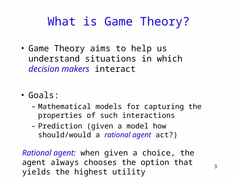
What is Game Theory?

• Game Theory aims to help us understand situations in which decision makers interact

• Goals:– Mathematical models for capturing the properties of

such interactions

– Prediction (given a model how should/would a rational agent act?)

Rational agent: when given a choice, the agent always chooses the option that yields the highest utility

4

Models of Games

• Cooperative or noncooperative

• Simultaneous moves or sequential

• Finite or infinite

• Complete information or incomplete information

5

In this talk:

• Cooperative or noncooperative

• Simultaneous moves or sequential

• Finite or infinite

• Complete information or incomplete information

6

Noncooperative Games in Normal Form

2, 2

0, 4

4, 0 -1, -1

Row

player

Column PlayerThe Hawk-Dove game

7

Example 2: The Bach or Stravinsky game (BoS)

2, 1

0, 0

0, 0 1, 2

8

Example 3: A Routing Game

● ● s t

A: 5x

B: 7.5x

C: 10x

9

Example 3: A Routing Game

10, 10

5, 7.5

5, 10

7.5, 5

15, 15

7.5, 10

10, 5 10, 7.5 20, 20

A B C

A

B

C

10

Definitions

• 2-player game (R, C):

• n available pure strategies for each player

• n x n payoff matrices R, C

• i, j played payoffs : Rij , Cij

• Mixed strategy: Probability distribution over [n]

• Expected payoffs :

11

Solution Concept

x*, y* is a Nash equilibrium if no player has a unilateral incentive to deviate:

(x, Ry*) (x*, Ry*) x

(x*, Cy) (x*, Cy*) y

[Nash, 1951]: Every finite game has a mixed strategy equilibrium.

Proof: Based on Brouwer’s fixed point theorem.

(think of it as a steady state)

12

Solution Concept

x*, y* is a Nash equilibrium if no player has a unilateral incentive to deviate:

(x, Ry*) (x*, Ry*) x

(x*, Cy) (x*, Cy*) y

[Nash, 1951]: Every finite game has a mixed strategy equilibrium.

Proof: Based on Brouwer’s fixed point theorem.

(think of it as a steady state)

13

Solution Concept

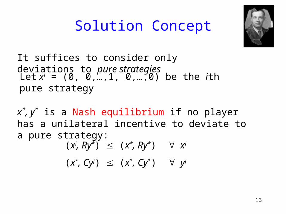
x*, y* is a Nash equilibrium if no player has a unilateral incentive to deviate to a pure strategy:

(xi, Ry*) (x*, Ry*) xi

(x*, Cyj) (x*, Cy*) yj

It suffices to consider only deviations to pure strategies

Let xi = (0, 0,…,1, 0,…,0) be the ith pure strategy

14

Example: The Hawk-Dove Game

2, 2

0, 4

4, 0 -1, -1

Row

player

Column Player

15

Example 2: The Bach or Stravinsky game (BoS)

2, 1

0, 0

0, 0 1, 2

3 equilibrium points:

1. (B, B)

2. (S, S)

3. ((2/3, 1/3), (1/3, 2/3))

16

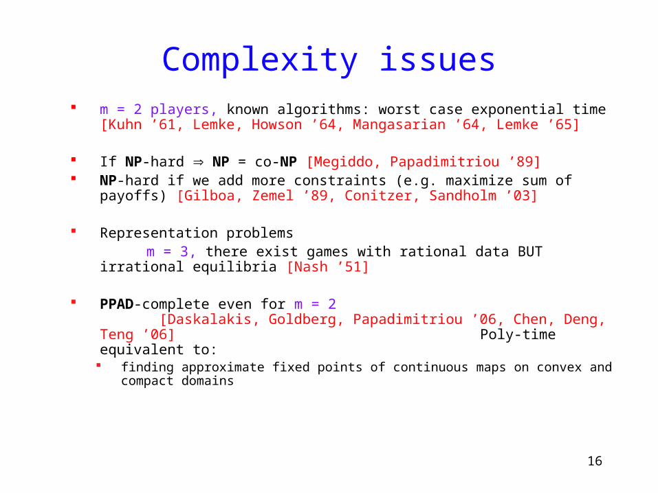
Complexity issues m = 2 players, known algorithms: worst case exponential time [Kuhn ’61,

Lemke, Howson ’64, Mangasarian ’64, Lemke ’65]

If NP-hard NP = co-NP [Megiddo, Papadimitriou ’89] NP-hard if we add more constraints (e.g. maximize sum of payoffs) [Gilboa,

Zemel ’89, Conitzer, Sandholm ’03]

Representation problems m = 3, there exist games with rational data BUT irrational equilibria [Nash ’51]

PPAD-complete even for m = 2 [Daskalakis, Goldberg, Papadimitriou ’06, Chen, Deng, Teng ’06] Poly-time equivalent to: finding approximate fixed points of continuous maps on convex and compact

domains

17

Approximate Nash Equilibria

• Recall definition of Nash eq. :

(x, Ry*) (x*, Ry*) x

(x*, Cy) (x*, Cy*) y

-Nash equilibria (incentive to deviate ) :

(x, Ry*) (x*, Ry*) + x

(x*, Cy) (x*, Cy*) + y

Normalization: entries of R, C in [0,1]

18

Searching for Approximate Equilibria

[Lipton, M., Mehta ’03]: For any in (0,1), and for every k 9logn/2, there exists a pair of k-uniform strategies x, y that form an -Nash equilibrium.

Definition: A k-uniform strategy is a strategy where all

probabilities are integer multiples of 1/k

e.g. (3/k, 0, 0, 1/k, 5/k, 0,…, 6/k)

19

A Subexponential Algorithm (Quasi-PTAS)

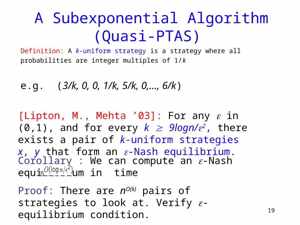
[Lipton, M., Mehta ’03]: For any in (0,1), and for every k 9logn/2, there exists a pair of k-uniform strategies x, y that form an -Nash equilibrium.

Definition: A k-uniform strategy is a strategy where all

probabilities are integer multiples of 1/k

e.g. (3/k, 0, 0, 1/k, 5/k, 0,…, 6/k)

Corollary : We can compute an -Nash equilibrium in time

Proof: There are nO(k) pairs of strategies to look at. Verify -equilibrium condition.

20

Proof of Existence

Let x*, y* be a Nash equilibrium.

- Sample k times from the set of pure strategies of the row player, independently, at random, according to x* k-uniform strategy x

- Same for column player k-uniform strategy y

Based on the probabilistic method (sampling)

Suffices to show Pr[x, y form an -Nash eq.] > 0

21

Proof (cont’d)

Enough to consider deviations to pure strategies

(xi, Ry) (x, Ry) + i

(xi, Ry): sum of k random variables with mean (xi, Ry*)

Chernoff-Hoeffding bounds (xi, Ry) (xi, Ry*) with high probability

(xi, Ry) (xi, Ry*) ≤ (x*, Ry*) (x, Ry)

Finally when k = (logn/2) :

Pr[ deviation with gain more than ] =

22

Multi-player Games

For m players, same technique:

support size: k = O(m2 log(m2 n)/2)

running time: exp(logn, m, 1/)

Previously [Scarf ’67]: exp(n, m, log(1/)) (fixed point approximation)

[Lipton, M. ’04]: exp(n, m) but poly(log(1/)) (using algorithms for polynomial equations)

23

Outline

Introduction to Games- The concepts of Nash and -Nash equilibrium

Computing approximate Nash equilibria

- A subexponential algorithm for any constant > 0

- Polynomial time approximation algorithms

Conclusions

24

Polynomial Time Approximation

Algorithms

For = 1/2:

Feder, Nazerzadeh, Saberi ’07: For < 1/2, we need support at least (log n)

i

k

j

• Pick arbitrary row i

• Let j = best response to i

• Find k = best response to j, play i or k with prob. 1/2

Rij, Cij

Rkj, Ckj

25

Polynomial Time Approximation

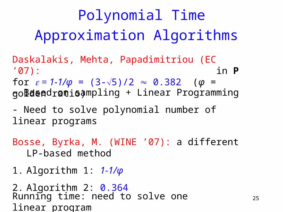
Algorithms Daskalakis, Mehta, Papadimitriou (EC ’07): in P for = 1-1/φ = (3-5)/2 0.382 (φ = golden ratio)

Bosse, Byrka, M. (WINE ’07): a different LP-based method

1. Algorithm 1: 1-1/φ

2. Algorithm 2: 0.364

- Βased on sampling + Linear Programming

- Need to solve polynomial number of linear programs

Running time: need to solve one linear program

26

Approach

Fact: 0-sum games can be solved in polynomial time (equivalent to linear programming)

- Start with an equilibrium of the 0-sum game (R-C, C-R)

- If incentives to deviate are “high”, players take turns and adjust their strategies via best response moves

0-sum games: games of the form (R, -R)

Similar idea used in [Kontogiannis, Spirakis ’07] for a different notion of approximation

27

Algorithm 1

1. Find an equilibrium x*, y* of the 0-sum game (R - C, C - R)

2. Let g1, g2 be the incentives to deviate for row and column player respectively. Suppose g1 g2

3. If g1 , output x*, y*

4. Else: let b1 = best response to y*, b2 = best response to b1

5. Output:

x = b1

y = (1 - 2) y* + 2 b2

Theorem: Algorithm 1 with = 1-1/φ and 2 = (1- g1) / (2- g1) achieves a (1-1/φ)-approximation

Parameters: , 2 [0,1]

28

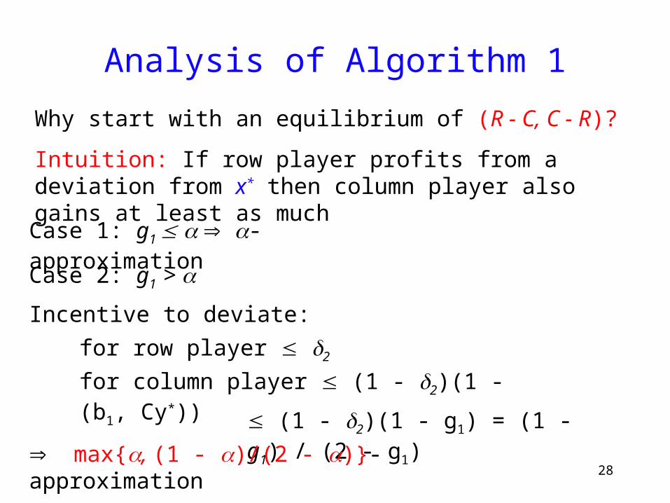
Analysis of Algorithm 1

Why start with an equilibrium of (R - C, C - R)?

Intuition: If row player profits from a deviation from x* then column player also gains at least as much

Case 1: g1 -approximation

Case 2: g1 >

for row player 2

for column player (1 - 2)(1 - (b1, Cy*))

(1 - 2)(1 - g1) = (1 - g1) / (2 - g1)

max{, (1 - )/(2 - )}-approximation

Incentive to deviate:

29

Analysis of Algorithm 1

30

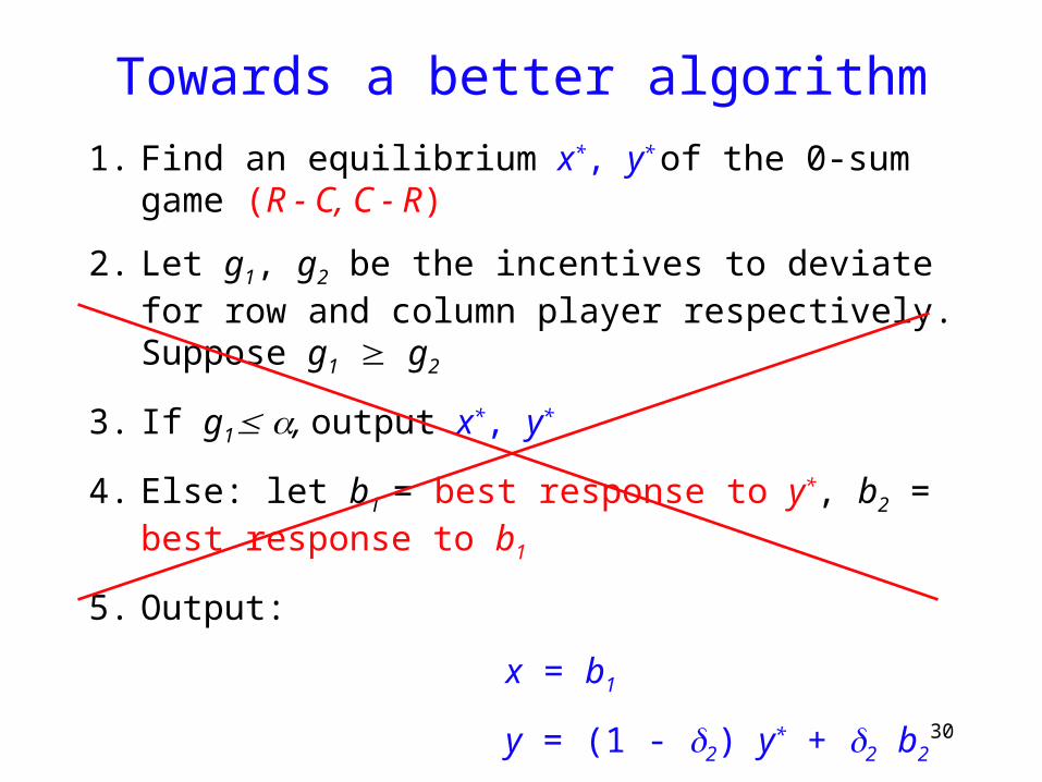
Towards a better algorithm

1. Find an equilibrium x*, y* of the 0-sum game (R - C, C - R)

2. Let g1, g2 be the incentives to deviate for row and column player respectively. Suppose g1 g2

3. If g1 , output x*, y*

4. Else: let b1 = best response to y*, b2 = best response to b1

5. Output:

x = b1

y = (1 - 2) y* + 2 b2

31

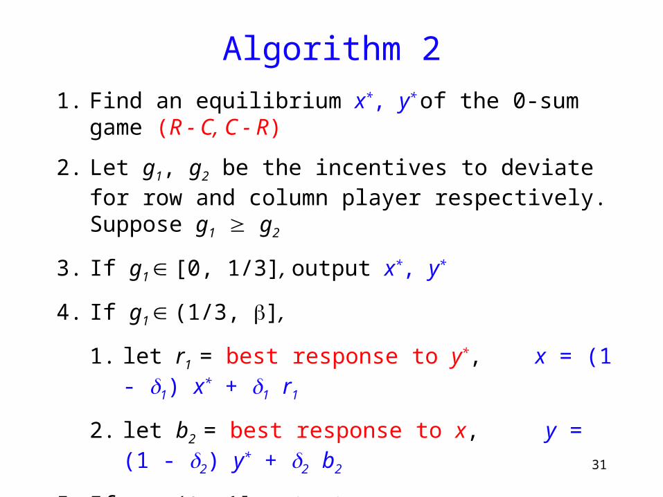
Algorithm 2

1. Find an equilibrium x*, y* of the 0-sum game (R - C, C - R)

2. Let g1, g2 be the incentives to deviate for row and column player respectively. Suppose g1 g2

3. If g1 [0, 1/3], output x*, y*

4. If g1 (1/3, ],

1. let r1 = best response to y*, x = (1 - 1) x* + 1 r1

2. let b2 = best response to x, y = (1 - 2) y* + 2 b2

5. If g1 (, 1] output:

x = r1

y = (1 - 2) y* + 2 b2

32

Analysis of Algorithm 2(Reducing to an optimization question)

- Let h = (x*, Cb2) - (x*, Cy*)

Theorem: The approximation guarantee of Algorithm 2 is 0.364 and is given by:

- We set 2 so as to equalize the incentives of the players to deviate

±2

33

Analysis of Algorithm 2 (solution)

Optimization yields:

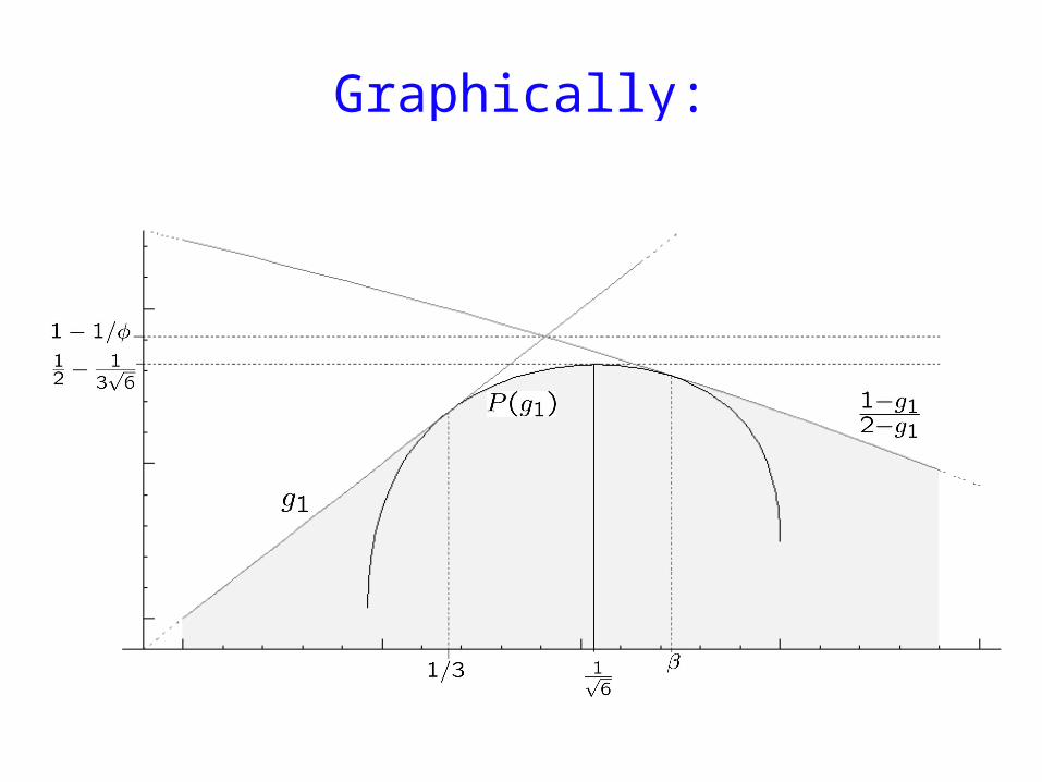
34

Graphically:

35

Analysis – tight example

0, 0 , ,

, 0, 1 1, 1/2

, 1, 1/2 0, 1

(R, C) =

=

36

Remarks and Open Problems

• Spirakis, Tsaknakis (WINE ’07): currently best approximation of 0.339 – yet another LP-based method

• Polynomial Time Approximation Scheme (PTAS)? Yes if:

– rank(R) = O(1) & rank(C) = O(1) [Lipton, M. Mehta ’03] – rank(R+C) = O(1) [Kannan, Theobald ’06]

• PPAD-complete for = 1/n [Chen, Deng, Teng ’06]

37

Other Notions of Approximation

-well-supported equilibria: every strategy in the support is an approximate best response– [Kontogiannis, Spirakis ’07]: 0.658-approximation, based

also on solving 0-sum games

• Strong approximation: output is geometrically close to an exact Nash equilibrium – [Etessami, Yannakakis ’07]: mostly negative results

38

Thank You!