Embed Size (px)
Citation preview
AERO0032-1, Aeroelasticity and Experimental Aerodynamics, Lecture 9
Lecture 9: Supersonic Aeroelasticity
G. Dimitriadis
Aeroelasticity
1
AERO0032-1, Aeroelasticity and Experimental Aerodynamics, Lecture 9 2
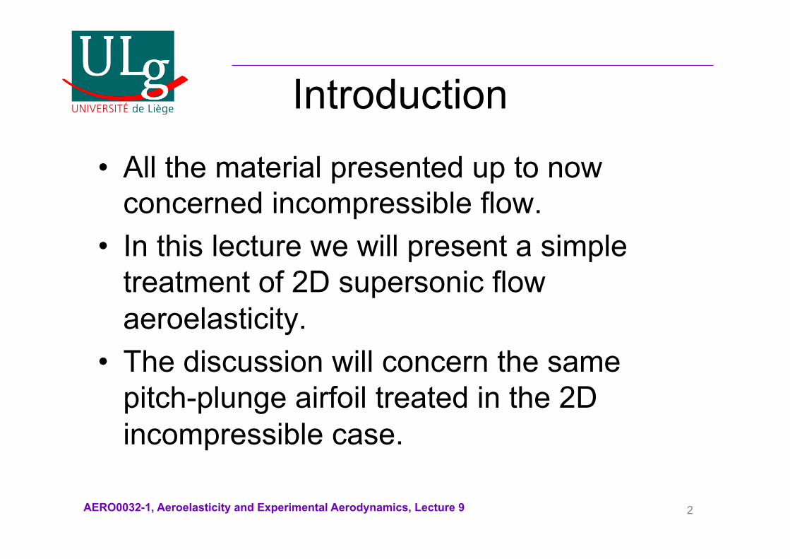
Introduction
• All the material presented up to now concerned incompressible flow.
• In this lecture we will present a simple treatment of 2D supersonic flow aeroelasticity.
• The discussion will concern the same pitch-plunge airfoil treated in the 2D incompressible case.
AERO0032-1, Aeroelasticity and Experimental Aerodynamics, Lecture 9 3
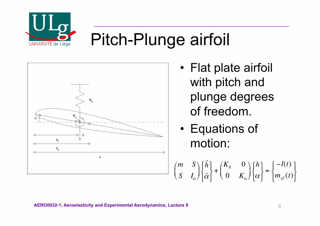
Pitch-Plunge airfoil • Flat plate airfoil
with pitch and plunge degrees of freedom.
• Equations of motion:
m SS Iα
#
$ %
&
' (
˙ ̇ h ˙ ̇ α
) * +
, - .
+Kh 00 Kα
#
$ %
&
' (
hα) * +
, - .
=−l(t)mxf (t)) * +
, - .
AERO0032-1, Aeroelasticity and Experimental Aerodynamics, Lecture 9 4
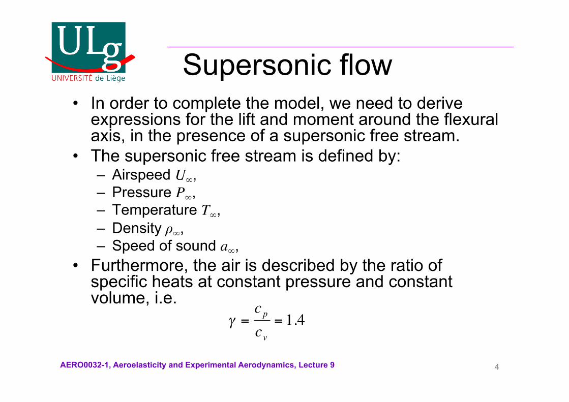
Supersonic flow • In order to complete the model, we need to derive
expressions for the lift and moment around the flexural axis, in the presence of a supersonic free stream.
• The supersonic free stream is defined by: – Airspeed U∞, – Pressure P∞, – Temperature T∞, – Density ρ∞, – Speed of sound a∞,
• Furthermore, the air is described by the ratio of specific heats at constant pressure and constant volume, i.e.
γ =cpcv
= 1.4
AERO0032-1, Aeroelasticity and Experimental Aerodynamics, Lecture 9 5
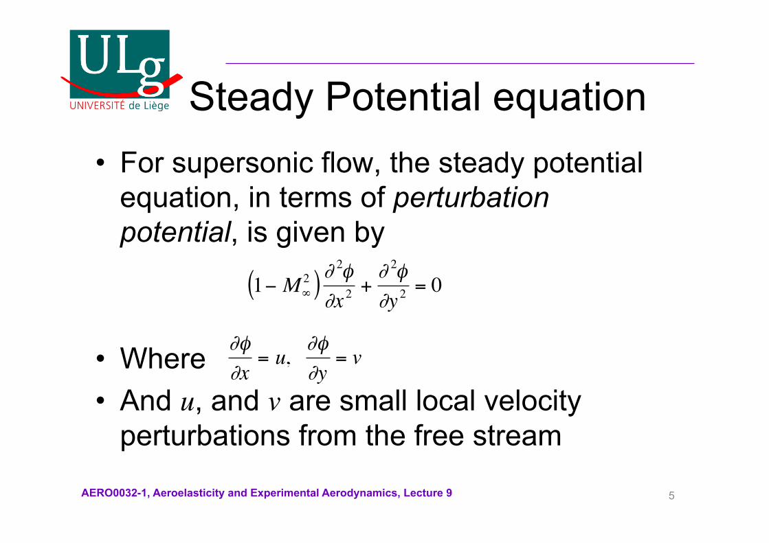
Steady Potential equation • For supersonic flow, the steady potential
equation, in terms of perturbation potential, is given by
• Where • And u, and v are small local velocity
perturbations from the free stream
1− M∞2( )∂
2φ∂x 2
+∂ 2φ∂y 2
= 0
∂φ∂x
= u, ∂φ∂y
= v
AERO0032-1, Aeroelasticity and Experimental Aerodynamics, Lecture 9 6
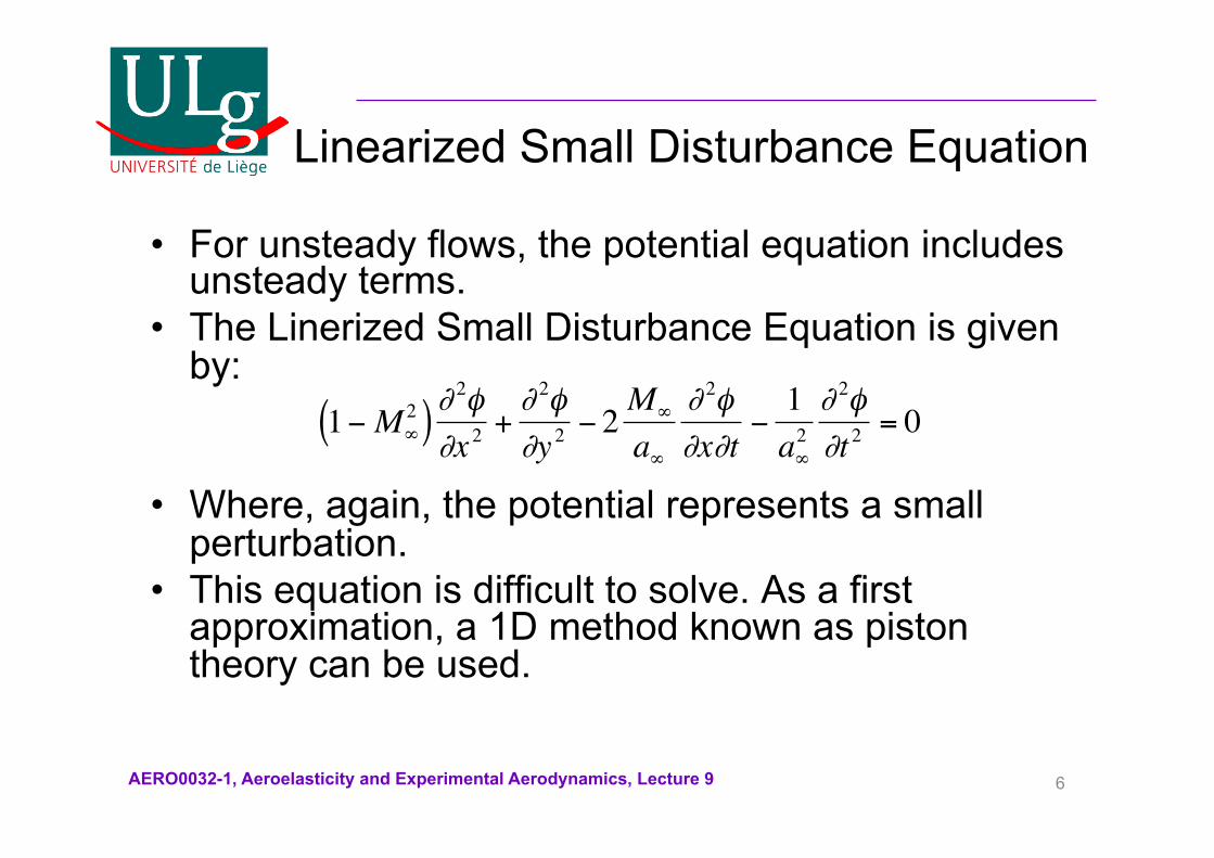
Linearized Small Disturbance Equation
• For unsteady flows, the potential equation includes unsteady terms.
• The Linerized Small Disturbance Equation is given by:
• Where, again, the potential represents a small perturbation.
• This equation is difficult to solve. As a first approximation, a 1D method known as piston theory can be used.
1−M∞2( )∂
2φ∂x 2
+∂ 2φ∂y 2
− 2 M∞
a∞
∂ 2φ∂x∂t
−1a∞2∂ 2φ∂t 2
= 0
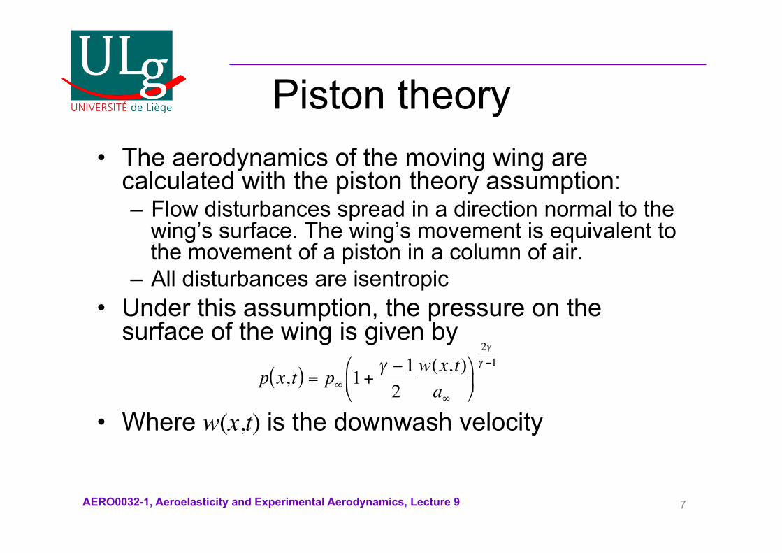
AERO0032-1, Aeroelasticity and Experimental Aerodynamics, Lecture 9 7
Piston theory • The aerodynamics of the moving wing are
calculated with the piston theory assumption: – Flow disturbances spread in a direction normal to the
wing’s surface. The wing’s movement is equivalent to the movement of a piston in a column of air.
– All disturbances are isentropic • Under this assumption, the pressure on the
surface of the wing is given by
• Where w(x,t) is the downwash velocity
p x, t( ) = p∞ 1+γ −12
w(x, t)a∞
%
& '
(
) *
2γγ −1
AERO0032-1, Aeroelasticity and Experimental Aerodynamics, Lecture 9 8
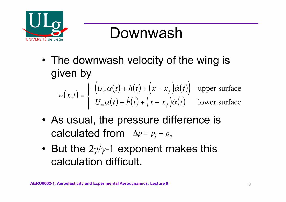
Downwash
• The downwash velocity of the wing is given by
• As usual, the pressure difference is calculated from
• But the 2γ/γ-1 exponent makes this calculation difficult.
w x, t( ) =− U∞α t( ) + ˙ h t( ) + x − x f( ) ˙ α t( )( ) upper surface
U∞α t( ) + ˙ h t( ) + x − x f( ) ˙ α t( ) lower surface
% & '
( '
Δp = pl − pu
AERO0032-1, Aeroelasticity and Experimental Aerodynamics, Lecture 9 9
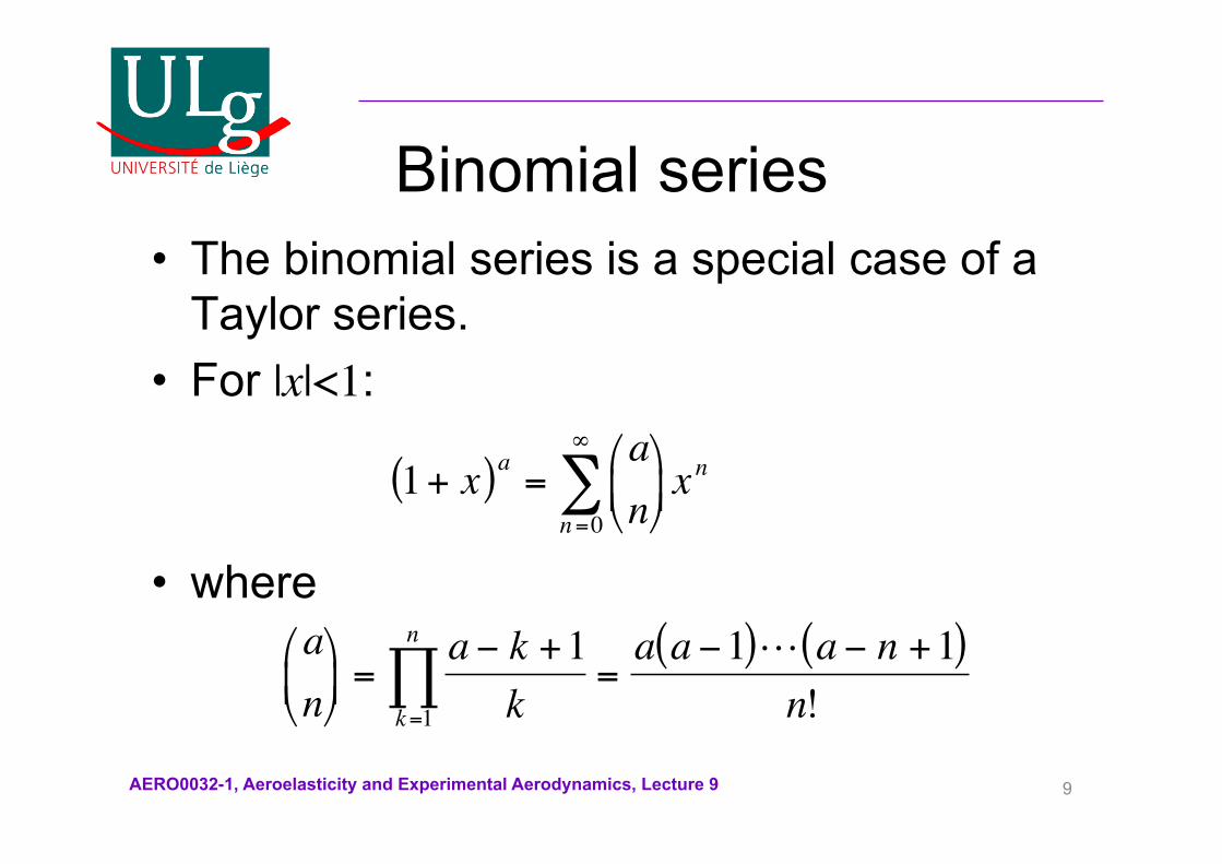
Binomial series • The binomial series is a special case of a
Taylor series. • For |x|<1:
• where
1+ x( )a =an"
# $ %
& ' xn
n=0
∞
∑
an"
# $ %
& ' =
a − k +1kk=1
n
∏ =a a −1( ) a − n +1( )
n!
AERO0032-1, Aeroelasticity and Experimental Aerodynamics, Lecture 9 10
Binomial expansion • Assume that the downwash velocity is much smaller
than the speed of sound, we can use a binomial series on the pressure equation:
• Where is a correction factor
• Retaining only the linear term leads to
p x, t( ) = p∞ 1+γ −12
w(x, t)a∞
#
$%
&
'(
2γγ−1
≈ p∞ 1+γwa∞λ +
γ γ +1( )4
wa∞
#
$%
&
'(
2
λ 2 +γ γ +1( )12
wa∞
#
$%
&
'(
3
λ3#
$%%
&
'((
p x, t( ) ≈ p∞ 1+γwa∞λ
#
$%
&
'(
λ =M∞
M∞2 −1
AERO0032-1, Aeroelasticity and Experimental Aerodynamics, Lecture 9 11
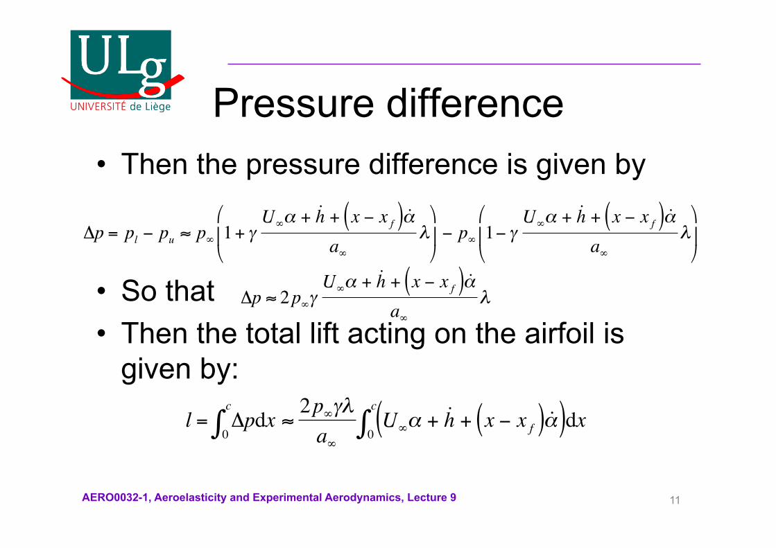
Pressure difference • Then the pressure difference is given by
• So that • Then the total lift acting on the airfoil is
given by:
Δp = pl − pu ≈ p∞ 1+ γU∞α + ˙ h + x − x f( ) ˙ α
a∞λ
)
* +
,
- . − p∞ 1− γ
U∞α + ˙ h + x − x f( ) ˙ α
a∞λ
)
* +
,
- .
Δp ≈ 2p∞γU∞α + ˙ h + x − x f( ) ˙ α
a∞λ
l = Δpdx0
c
∫ ≈2p∞γλ
a∞U∞α + ˙ h + x − x f( ) ˙ α ( )dx
0
c
∫
AERO0032-1, Aeroelasticity and Experimental Aerodynamics, Lecture 9 12
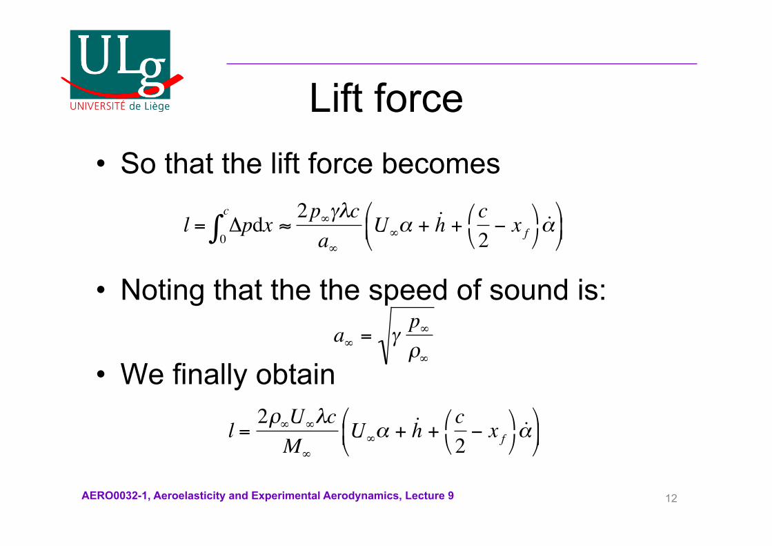
Lift force • So that the lift force becomes
• Noting that the the speed of sound is: • We finally obtain
l = Δpdx0
c
∫ ≈2p∞γλc
a∞U∞α + ˙ h +
c2− x f
* +
, -
˙ α * + .
, - /
a∞ = γp∞ρ∞
l =2ρ∞U∞λc
M∞
U∞α + ˙ h +c2− x f
' (
) *
˙ α ' ( +
) * ,
AERO0032-1, Aeroelasticity and Experimental Aerodynamics, Lecture 9 13
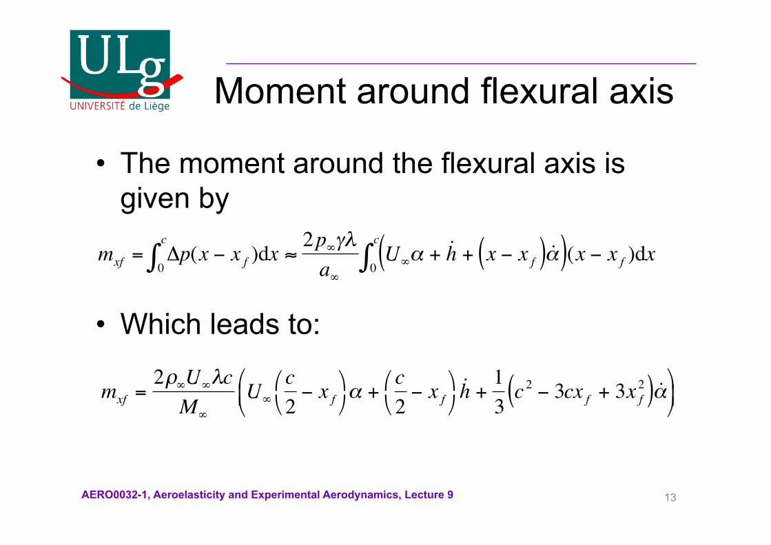
Moment around flexural axis
• The moment around the flexural axis is given by
• Which leads to:
mxf = Δp(x − x f )dx0
c
∫ ≈2p∞γλ
a∞U∞α + ˙ h + x − x f( ) ˙ α ( )(x − x f )dx
0
c
∫
mxf =2ρ∞U∞λc
M∞
U∞
c2− x f
& '
( ) α +
c2− x f
& '
( )
˙ h +13
c 2 − 3cx f + 3x f2( ) ˙ α
& ' +
( ) ,
AERO0032-1, Aeroelasticity and Experimental Aerodynamics, Lecture 9 14
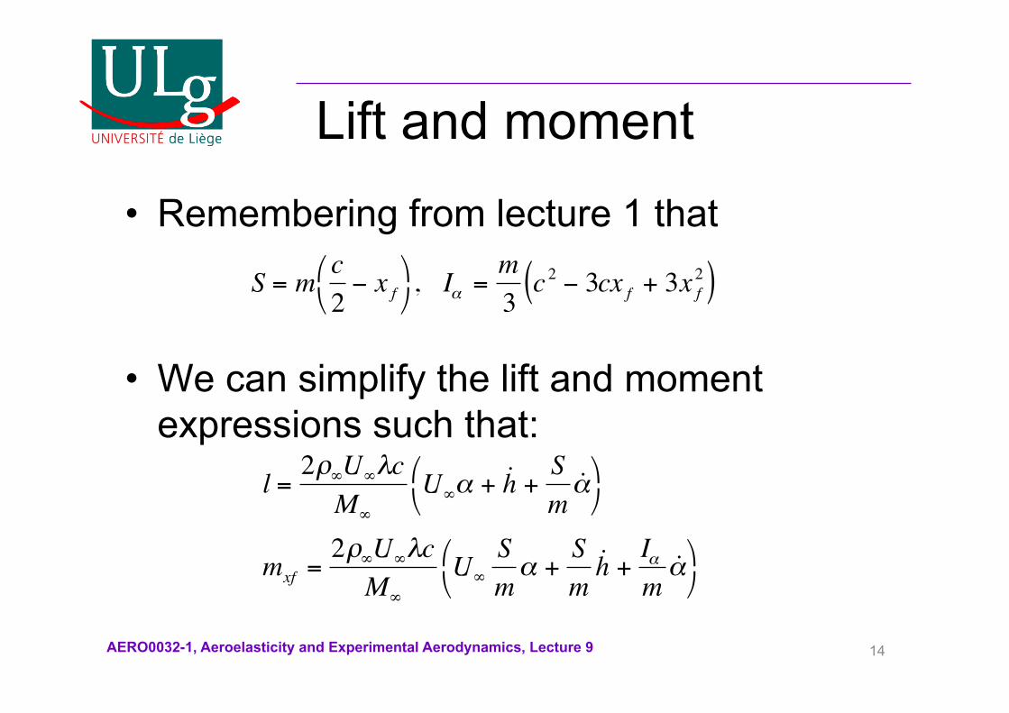
Lift and moment • Remembering from lecture 1 that
• We can simplify the lift and moment expressions such that:
S = mc2− x f
# $
% & , Iα =
m3c 2 − 3cx f + 3x f
2( )
l =2ρ∞U∞λc
M∞
U∞α + ˙ h +Sm
˙ α & '
( )
mxf =2ρ∞U∞λc
M∞
U∞
Smα +
Sm
˙ h +Iαm
˙ α & '
( )
AERO0032-1, Aeroelasticity and Experimental Aerodynamics, Lecture 9 15
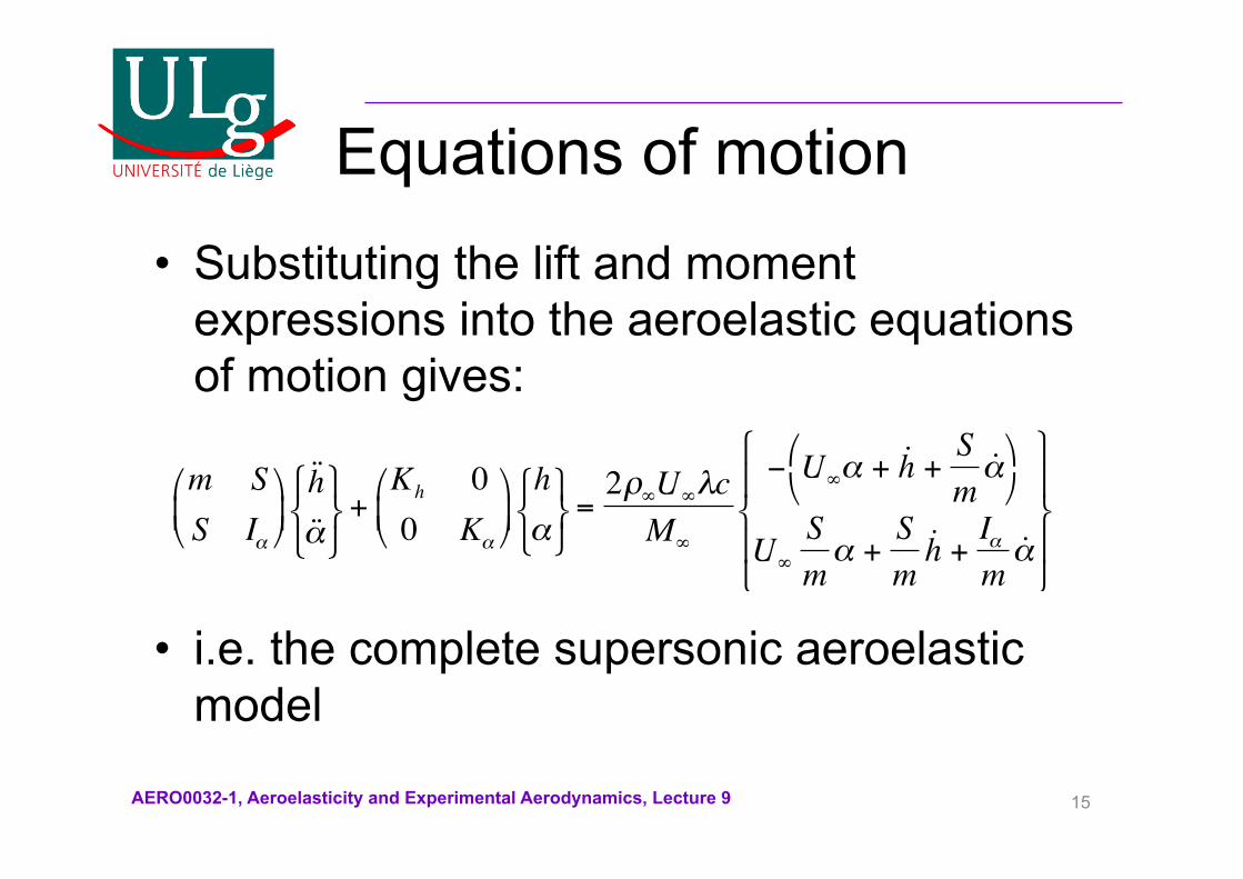
Equations of motion • Substituting the lift and moment
expressions into the aeroelastic equations of motion gives:
• i.e. the complete supersonic aeroelastic model
m SS Iα#
$ %
&
' (
˙ ̇ h ˙ ̇ α
) * +
, - .
+Kh 00 Kα
#
$ %
&
' (
hα) * +
, - .
=2ρ∞U∞λc
M∞
− U∞α + ˙ h + Sm
˙ α # $
& '
U∞
Smα +
Sm
˙ h + Iαm
˙ α
)
* 3
+ 3
,
- 3
. 3
AERO0032-1, Aeroelasticity and Experimental Aerodynamics, Lecture 9 16
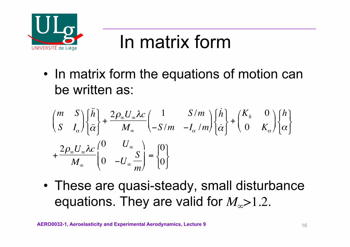
In matrix form • In matrix form the equations of motion can
be written as:
• These are quasi-steady, small disturbance equations. They are valid for M∞>1.2.
m SS Iα#
$ %
&
' (
˙ ̇ h ˙ ̇ α
) * +
, - .
+2ρ∞U∞λc
M∞
1 S /m−S /m −Iα /m#
$ %
&
' (
˙ h ˙ α
) * +
, - .
+Kh 00 Kα
#
$ %
&
' (
hα) * +
, - .
+2ρ∞U∞λc
M∞
0 U∞
0 −U∞
Sm
#
$ % %
&
' ( (
=00) * +
, - .
AERO0032-1, Aeroelasticity and Experimental Aerodynamics, Lecture 9 17
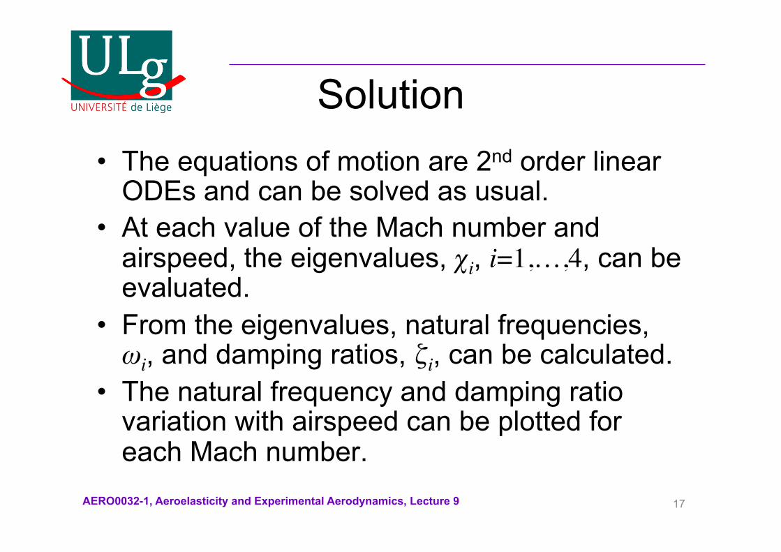
Solution • The equations of motion are 2nd order linear
ODEs and can be solved as usual. • At each value of the Mach number and
airspeed, the eigenvalues, χi, i=1,…,4, can be evaluated.
• From the eigenvalues, natural frequencies, ωi, and damping ratios, ζi, can be calculated.
• The natural frequency and damping ratio variation with airspeed can be plotted for each Mach number.
AERO0032-1, Aeroelasticity and Experimental Aerodynamics, Lecture 9 18
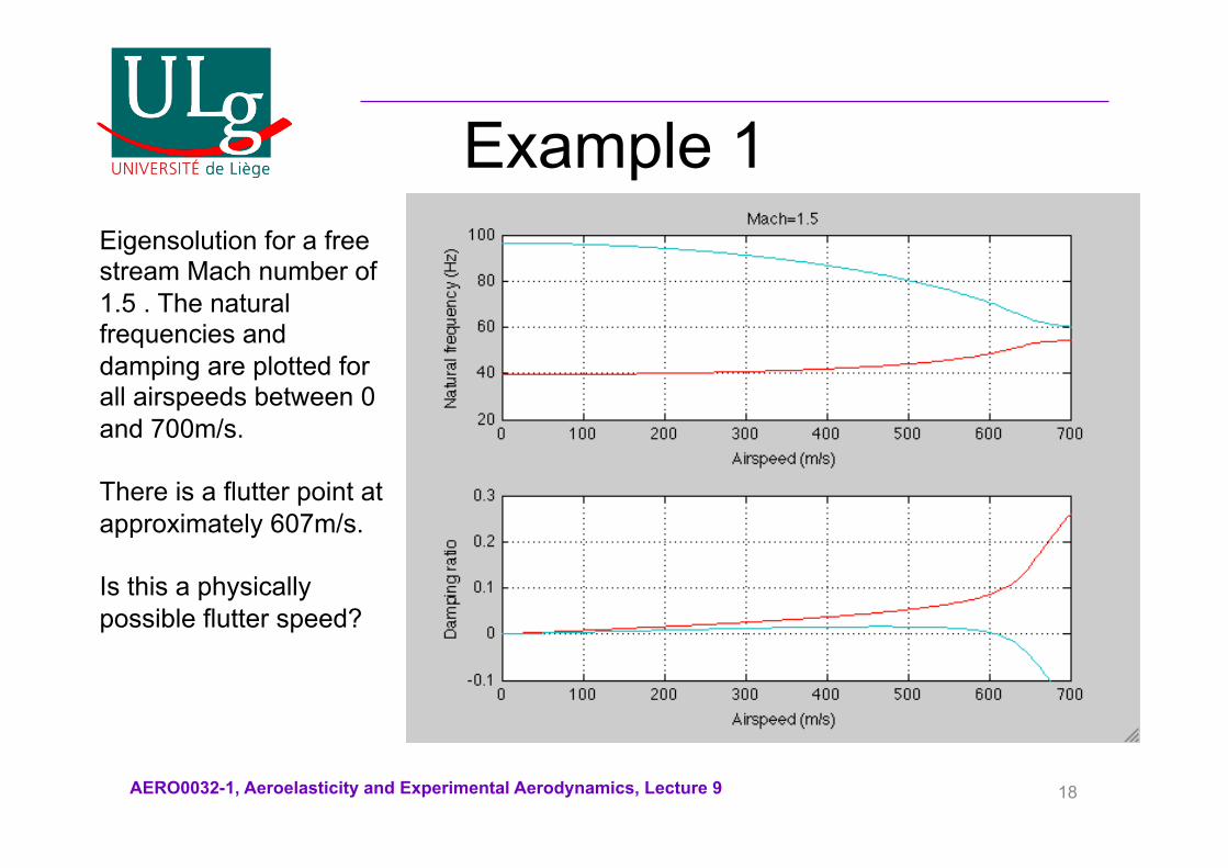
Example 1 Eigensolution for a free stream Mach number of 1.5 . The natural frequencies and damping are plotted for all airspeeds between 0 and 700m/s. There is a flutter point at approximately 607m/s. Is this a physically possible flutter speed?
AERO0032-1, Aeroelasticity and Experimental Aerodynamics, Lecture 9 19
Unmatched flutter speeds • The flutter speed calculated in this example may or may
not be physical, it depends on the system’s flight condition.
• Consider the case where the wing is flying at sea level and the atmospheric pressure is 1bar: – ρ∞=1.225kg/m3
– p∞=101325Pa • Then the speed of sound is 340m/s. Therefore, the flutter
speed of 607m/s corresponds to a Mach number of 1.8. • But the Mach number used for the simulation is 1.5. This
case is an example of an unmatched flutter speed. The system can flutter but not at an attainable Mach number.
• As the flutter Mach number is higher than the simulation Mach number, this is a safe flight condition.
AERO0032-1, Aeroelasticity and Experimental Aerodynamics, Lecture 9 20
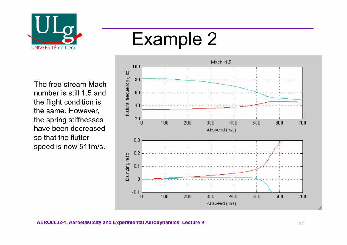
Example 2
The free stream Mach number is still 1.5 and the flight condition is the same. However, the spring stiffnesses have been decreased so that the flutter speed is now 511m/s.
AERO0032-1, Aeroelasticity and Experimental Aerodynamics, Lecture 9 21
Matched flutter speed • The speed of sound is still 340m/s.
However, the new flutter speed is 511m/s. • This flutter speed occurs at a Mach
number of 1.5, the same as the simulation Mach number.
• This is an example of a matched flutter speed: flutter occurs at the simulation Mach number.
• Clearly the flight condition is not safe.
AERO0032-1, Aeroelasticity and Experimental Aerodynamics, Lecture 9 22
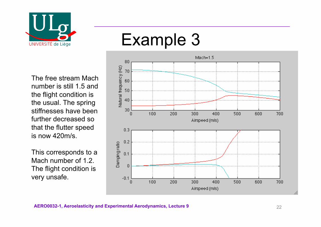
Example 3
The free stream Mach number is still 1.5 and the flight condition is the usual. The spring stiffnesses have been further decreased so that the flutter speed is now 420m/s. This corresponds to a Mach number of 1.2. The flight condition is very unsafe.
AERO0032-1, Aeroelasticity and Experimental Aerodynamics, Lecture 9 23
International Standard Atmosphere
• According to the equations of motion, the aerodynamic forces depend on the Mach number, flight speed and air density.
• The air density is a function of the flight altitude. • The altitude also defines the speed of sound.
Therefore, the aerodynamic forces only depend on flight altitude and flight Mach number.
• The International Standard Atmosphere determines the variation of density and speed of sound with altitude from sea level.
AERO0032-1, Aeroelasticity and Experimental Aerodynamics, Lecture 9 24
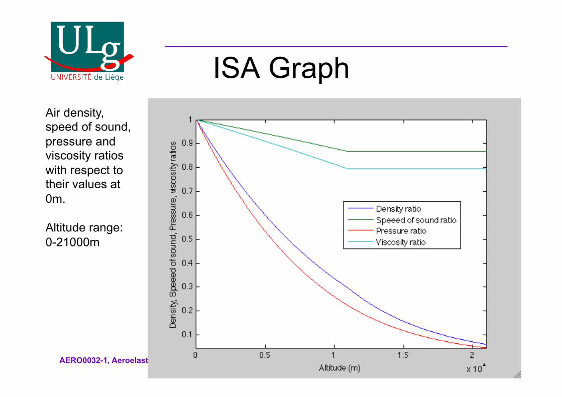
ISA Graph Air density, speed of sound, pressure and viscosity ratios with respect to their values at 0m. Altitude range:0-21000m
AERO0032-1, Aeroelasticity and Experimental Aerodynamics, Lecture 9 25
Mach-Airspeed diagrams
• For each Mach number and altitude, the flutter speed can be determined.
• This calculation will give rise to Mach-Airspeed diagrams for all flight conditions of interest.
• The diagrams will feature a flutter speed curve and a true airspeed curve.
• All flight conditions for which the true airspeed lies below the flutter speed are safe.
• All others are unsafe.
AERO0032-1, Aeroelasticity and Experimental Aerodynamics, Lecture 9 26
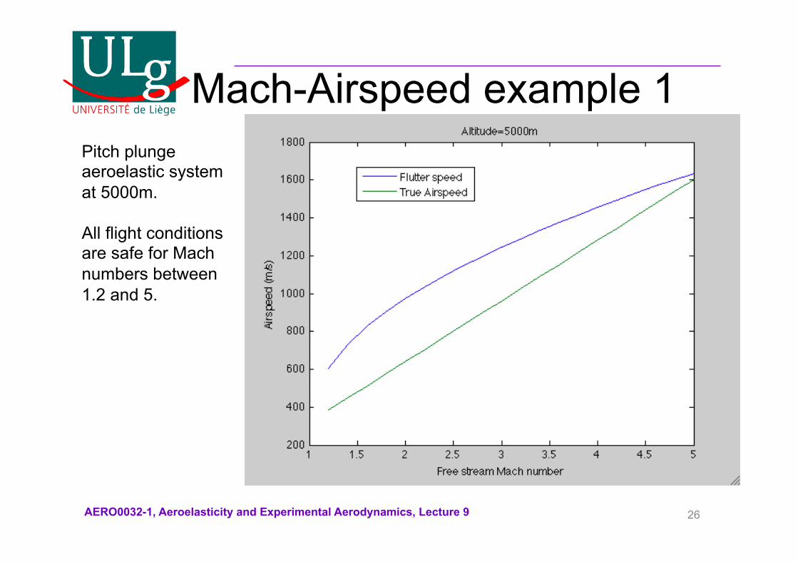
Mach-Airspeed example 1 Pitch plunge aeroelastic system at 5000m. All flight conditions are safe for Mach numbers between 1.2 and 5.
AERO0032-1, Aeroelasticity and Experimental Aerodynamics, Lecture 9 27
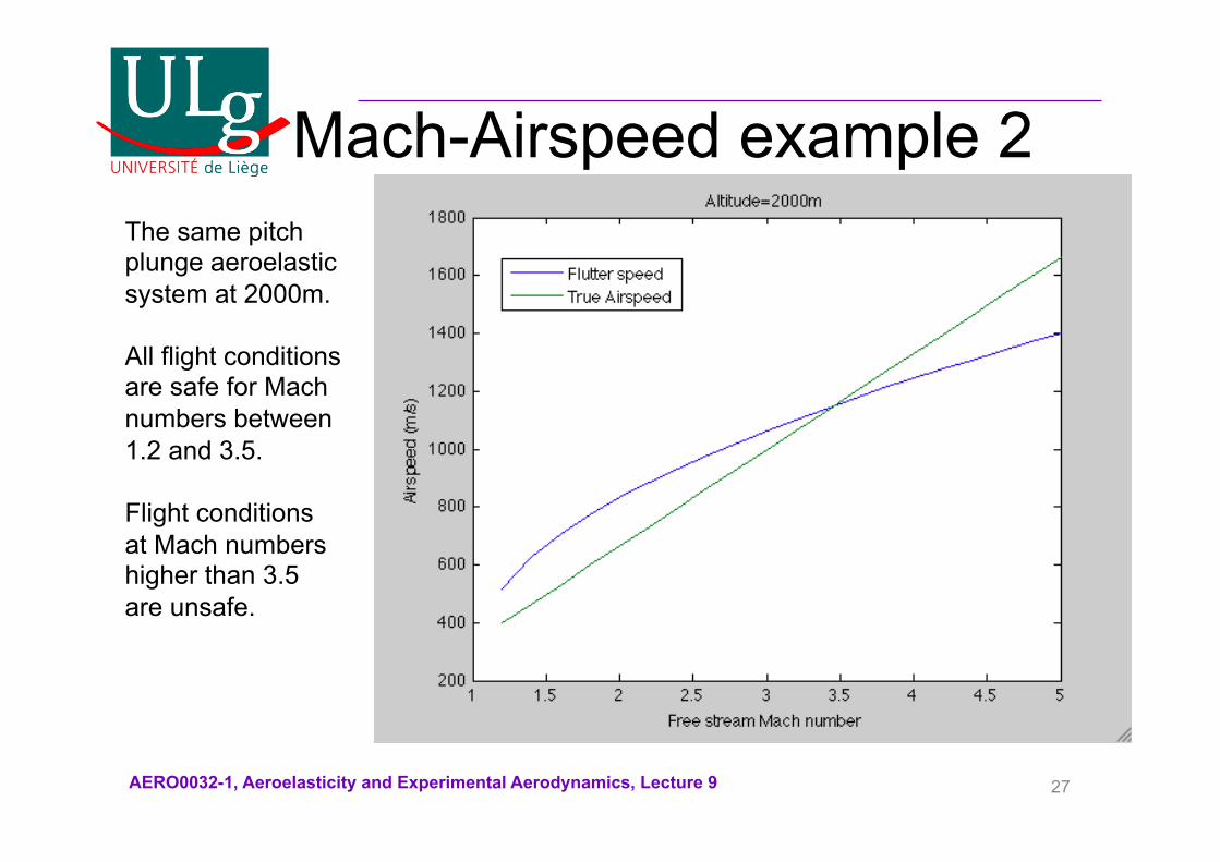
Mach-Airspeed example 2 The same pitch plunge aeroelastic system at 2000m. All flight conditions are safe for Mach numbers between 1.2 and 3.5. Flight conditions at Mach numbers higher than 3.5 are unsafe.
AERO0032-1, Aeroelasticity and Experimental Aerodynamics, Lecture 9 28
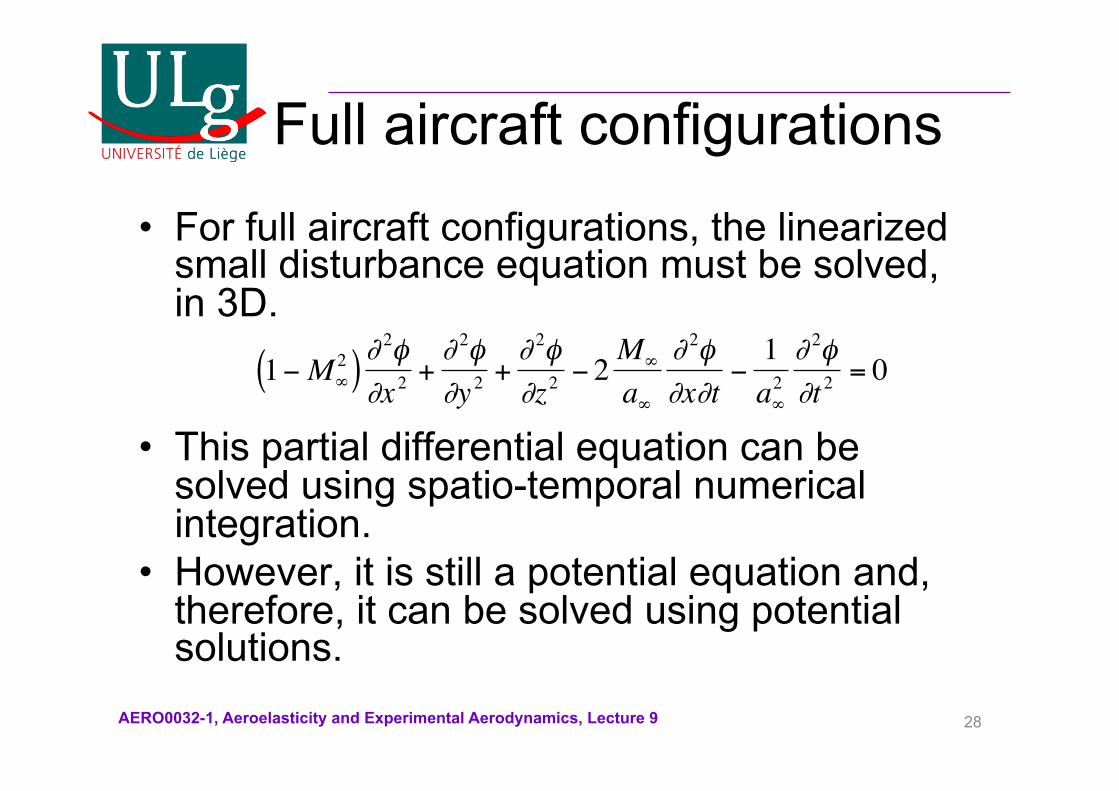
Full aircraft configurations • For full aircraft configurations, the linearized
small disturbance equation must be solved, in 3D.
• This partial differential equation can be solved using spatio-temporal numerical integration.
• However, it is still a potential equation and, therefore, it can be solved using potential solutions.
1−M∞2( )∂
2φ∂x 2
+∂ 2φ∂y 2
+∂ 2φ∂z2
− 2 M∞
a∞
∂ 2φ∂x∂t
−1a∞2∂ 2φ∂t 2
= 0
AERO0032-1, Aeroelasticity and Experimental Aerodynamics, Lecture 9 29
Sub/Supersonic panel methods
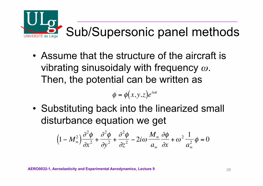
• Assume that the structure of the aircraft is vibrating sinusoidaly with frequency ω. Then, the potential can be written as
• Substituting back into the linearized small disturbance equation we get
φ = φ x,y,z( )eiωt
1−M∞2( )∂
2φ∂x 2
+∂ 2φ∂y 2
+∂ 2φ∂z2
− 2iω M∞
a∞
∂φ∂x
+ω 2 1a∞2 φ = 0
AERO0032-1, Aeroelasticity and Experimental Aerodynamics, Lecture 9 30
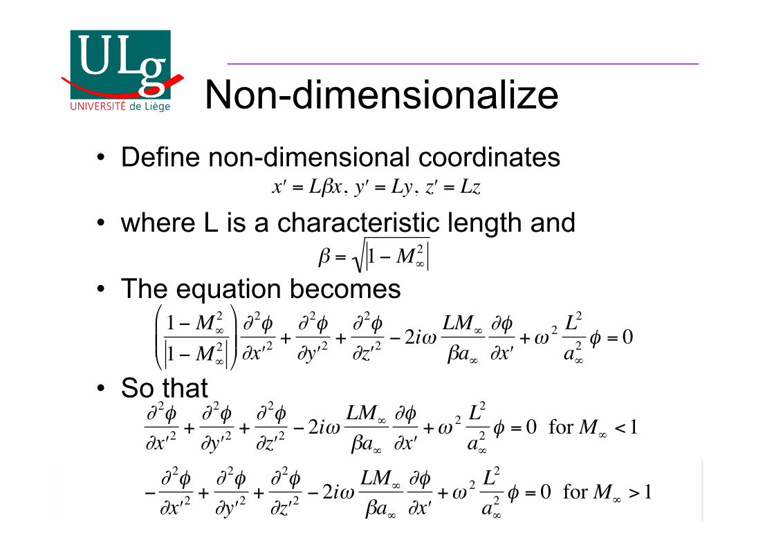
Non-dimensionalize • Define non-dimensional coordinates
• where L is a characteristic length and
• The equation becomes
• So that
" x = Lβx, " y = Ly, " z = Lz
β = 1−M∞2
1− M∞2
1− M∞2
$
% & &
'
( ) ) ∂ 2φ∂ , x 2
+∂ 2φ∂ , y 2
+∂ 2φ∂ , z 2
− 2iωLM∞
βa∞
∂φ∂ , x
+ω 2 L2
a∞2 φ = 0
∂ 2φ∂ $ x 2 +
∂ 2φ∂ $ y 2 +
∂ 2φ∂ $ z 2
− 2iωLM∞
βa∞
∂φ∂ $ x
+ω 2 L2
a∞2 φ = 0 for M∞ <1
−∂ 2φ∂ $ x 2 +
∂ 2φ∂ $ y 2 +
∂ 2φ∂ $ z 2
− 2iωLM∞
βa∞
∂φ∂ $ x
+ω 2 L2
a∞2 φ = 0 for M∞ >1
AERO0032-1, Aeroelasticity and Experimental Aerodynamics, Lecture 9 31
Modified potential • Furthermore, define a modified potential
such that
• Where ν is the compressible reduced frequency given by
• Then we obtain:
φ # x , # y , # z ( ) = φ # x , # y , # z ( )eiνM ∞ # x
ν =kM∞
β, and k =
ωLU∞
∂ 2φ ∂ $ x 2 +
∂ 2φ ∂ $ y 2 +
∂ 2φ ∂ $ z 2
+ν 2φ = 0 for M∞ <1
∂ 2φ ∂ $ x 2 −
∂ 2φ ∂ $ y 2 −
∂ 2φ ∂ $ z 2
+ν 2φ = 0 for M∞ >1
AERO0032-1, Aeroelasticity and Experimental Aerodynamics, Lecture 9 32
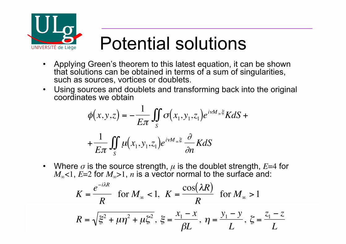
Potential solutions • Applying Green’s theorem to this latest equation, it can be shown
that solutions can be obtained in terms of a sum of singularities, such as sources, vortices or doublets.
• Using sources and doublets and transforming back into the original coordinates we obtain
• Where σ is the source strength, μ is the doublet strength, E=4 for M∞<1, E=2 for M∞>1, n is a vector normal to the surface and:
φ x,y,z( ) = −1Eπ
σS∫∫ x1,y1,z1( )eiνM ∞ξKdS +
+1Eπ
µS∫∫ x1,y1,z1( )eiνM ∞ξ
∂∂nKdS
K =e−iλR
R for M∞ <1, K =
cos λR( )R
for M∞ >1
R = ξ2 + µη2 + µζ2 , ξ =x1 − xβL
, η =y1 − yL
, ζ =z1 − zL
AERO0032-1, Aeroelasticity and Experimental Aerodynamics, Lecture 9 33
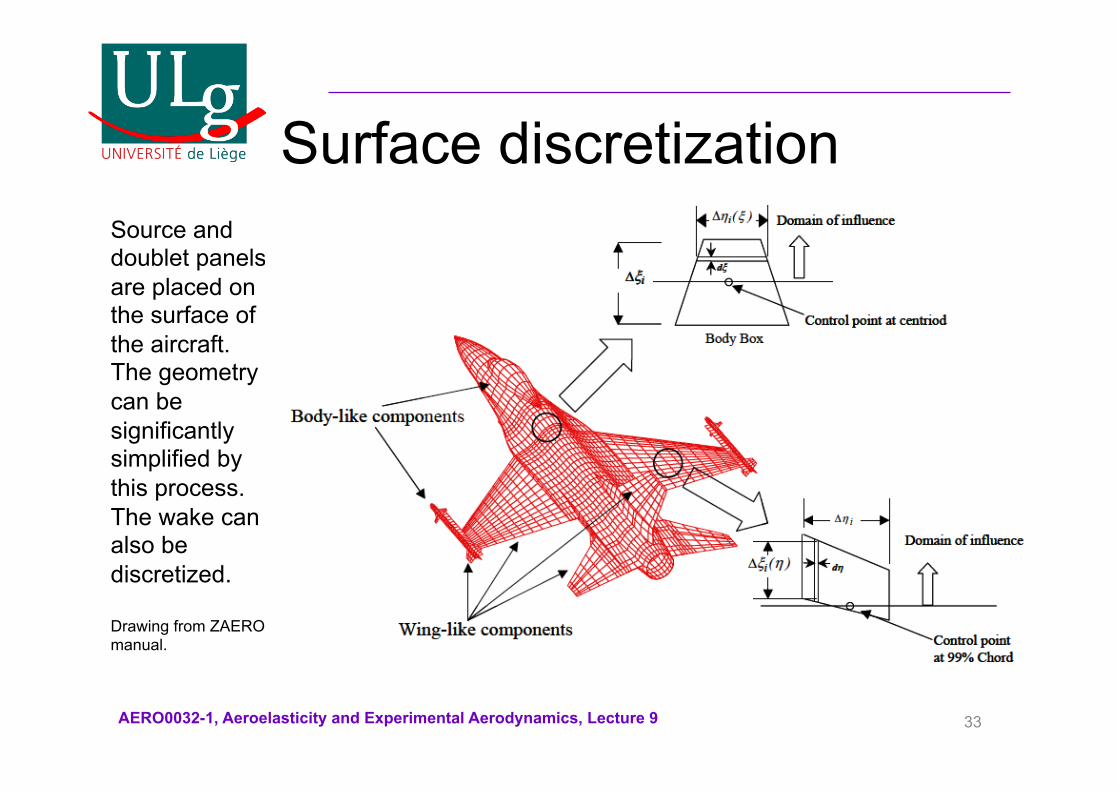
Surface discretization Source and doublet panels are placed on the surface of the aircraft. The geometry can be significantly simplified by this process. The wake can also be discretized. Drawing from ZAERO manual.
AERO0032-1, Aeroelasticity and Experimental Aerodynamics, Lecture 9 34
Boundary conditions • The source and doublet strengths are
obtained from the application of the non-penetration boundary condition over the complete surface of the aircraft.
• This boundary condition is unsteady, since the aircraft structure is vibrating.
• It can be written in terms of the modal displacements of the structure. In this case, the complete unsteady aerodynamic forces can be written in modal space.
AERO0032-1, Aeroelasticity and Experimental Aerodynamics, Lecture 9 35
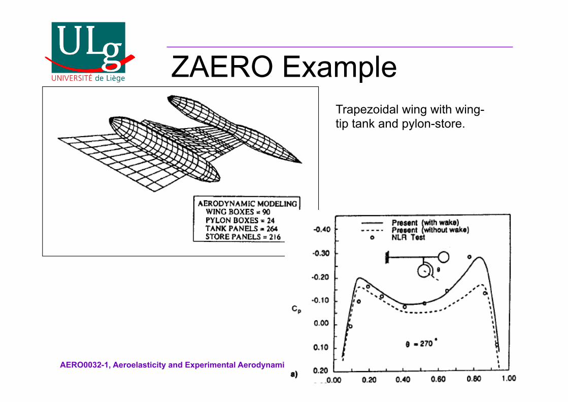
ZAERO Example Trapezoidal wing with wing-tip tank and pylon-store.
AERO0032-1, Aeroelasticity and Experimental Aerodynamics, Lecture 9 36
Discussion • This full aircraft approach is satisfactory for both
subsonic and supersonic aeroelastic problems. • However, at transonic flight conditions, the
aerodynamics become very complicated. Shock waves can oscillate on the wing surfaces, introducing nonlinearity and causing Limit Cycle Oscillations.
• Furthermore, the oscillating shock waves can interact with the boundary layer, forcing its separation. Even higher levels of nonlinearity can be generated.
• Under these circumstances, linearized methods cannot be applied and higher fidelity aerodynamic modelling is required.
AERO0032-1, Aeroelasticity and Experimental Aerodynamics, Lecture 9 37
Conclusions • Practical aeroelastic calculations for full
aircraft configurations are carried out using panel methods, whether subsonic or supersonic.
• Higher fidelity methods exist but they are reserved for challenging flowfields, such as transonic flow.
• Even so, they are very computationally expensive and are not routinely used for aircraft design purposes.