09 Exploration

7/28/2019 09 Exploration

http://slidepdf.com/reader/full/09-exploration 1/14

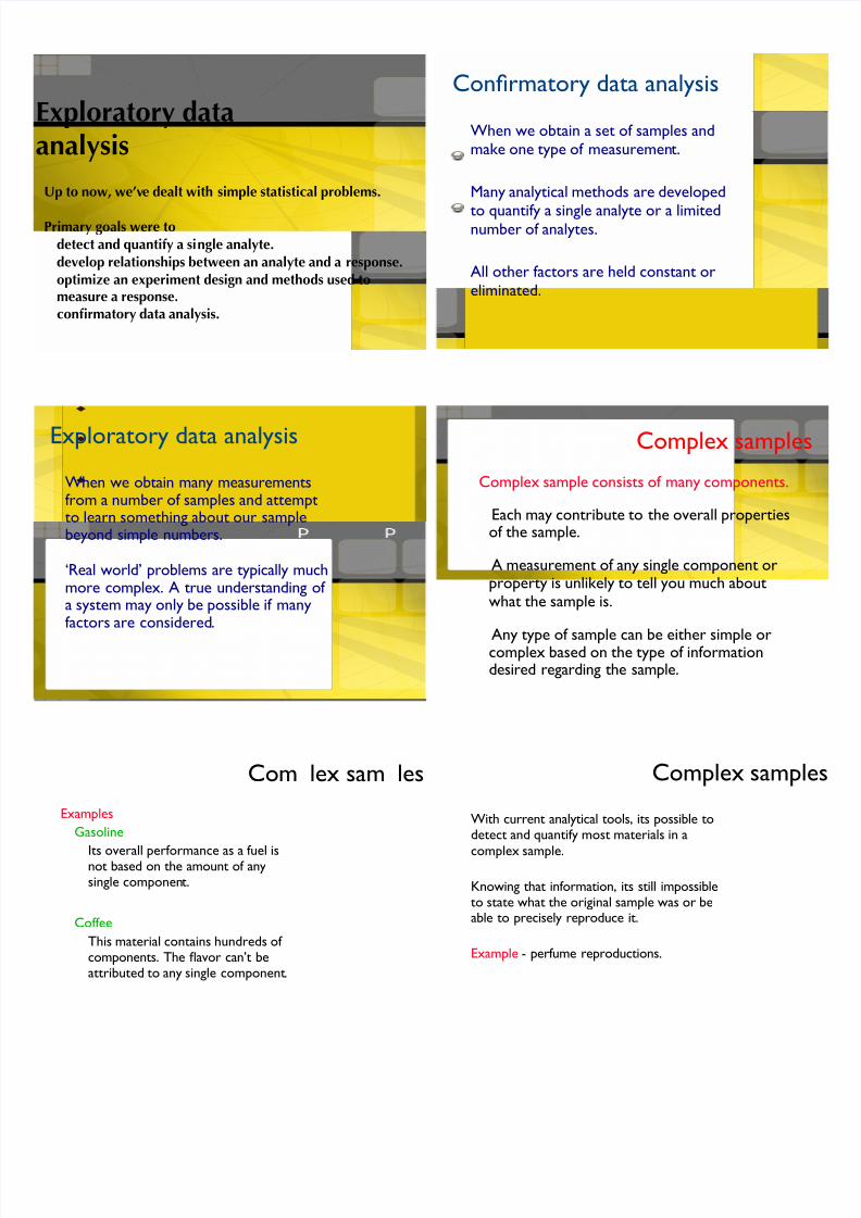
Exploratory dataanalysis

Up to now, we’ve dealt with simple statistical problems.

Primary goals were todetect and quantify a single analyte.develop relationships between an analyte and a response.optimize an experiment design and methods used tomeasure a response.confirmatory data analysis.

Confirmatory data analysis

When we obtain a set of samples andmake one type of measurement.

Many analytical methods are developed

to quantify a single analyte or a limitednumber of analytes.

All other factors are held constant or

eliminated.

Exploratory data analysis

When we obtain many measurementsfrom a number of samples and attemptto learn something about our samplebeyond simple numbers.

‘Real world’ problems are typically muchmore complex. A true understanding of a system may only be possible if manyfactors are considered.

Complex samples

Complex sample consists of many components.

Each may contribute to the overall propertiesof the sample.

A measurement of any single component orproperty is unlikely to tell you much aboutwhat the sample is.

Any type of sample can be either simple orcomplex based on the type of informationdesired regarding the sample.

Com lex sam les

Examples

Gasoline

Its overall performance as a fuel isnot based on the amount of anysingle component.

Coffee

This material contains hundreds of components. The flavor can’t beattributed to any single component.

Complex sampl

With current analytical tools, its possible todetect and quantify most materials in a

complex sample.

Knowing that information, its still impossibleto state what the original sample was or beable to precisely reproduce it.

Example - perfume reproductions.



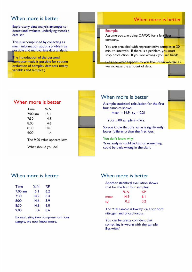
When more is better

Exploratory data analysis attempts to

detect and evaluate underlying trends a

data set.

This is accomplished by collecting as

much information about a problem aspossible and multivariate data analysis.

The introduction of the personal

computer made it possible for routine

evaluation of complex data sets (many

variables and samples.)

When more is better

Example.

Assume you are doing QA/QC for a fertilizer

company.

You are provided with representative samples at 30minute intervals. If there is a problem, you muststop production. If you are wrong - you are fired!

Let’s see what happens to you level of knowledge a

we increase the amount of data.

When more is better

Time! ! % N

7:00 am! 15.1

7:30! ! 14.9

8:00! ! 14.6

8:30! ! 14.8

9:00! ! 1.4

The 9:00 value appears low.

What should you do?

When more is betterA simple statistical calculation for the first

four samples shows:! ! mean = 14.9, sx = 0.21

! Your 9:00 sample is -9.6 s.

So you know that the value is significantly

lower (different) than the first four.

You don’t know why!

Your analysis could be bad or somethingcould be truly wrong in the plant.

When more is better

Time! ! % N! %P

7:00 am! 15.1! 6.27:30! ! 14.9! 6.4

8:00! ! 14.6! 5.9

8:30! ! 14.8! 6.0

9:00! ! 1.4! 0.6

By evaluating two components in our

sample, we now know more.

When more is better

Another statistical evaluation shows

that for the first four samples:

! ! ! % N! %P

mean! ! 14.9! ! 6.1

sx! ! ! 0.2! ! 0.2

The 9:00 sample is low by 9.6 s for both

nitrogen and phosphorous.

You can be pretty confident that

something is wrong with the sample.

But what?



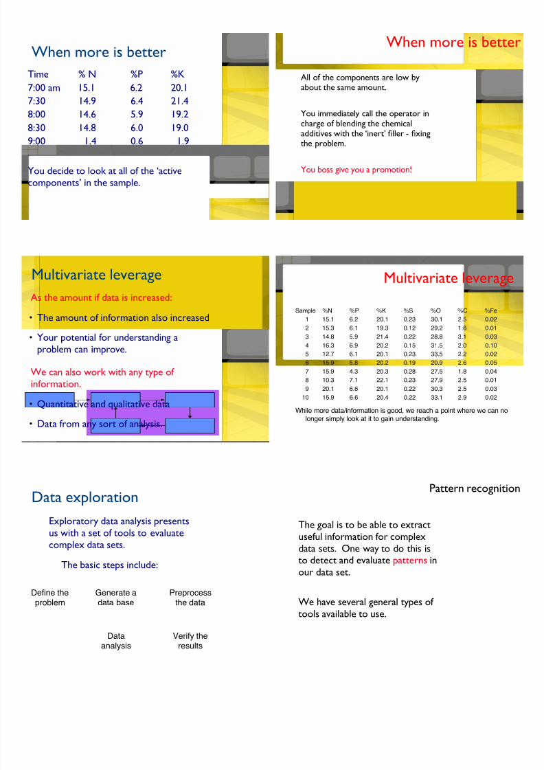
When more is better

Time! ! % N! ! %P %K

7:00 am! 15.1! 6.2 20.1

7:30! ! 14.9! ! 6.4 21.4

8:00! ! 14.6! ! 5.9 19.2

8:30! ! 14.8! ! 6.0 19.0

9:00! ! 1.4! ! 0.6 1.9

You decide to look at all of the ‘active

components’ in the sample.

When more is bette

All of the components are low byabout the same amount.

You immediately call the operator incharge of blending the chemical

additives with the ‘inert’ filler - fixingthe problem.

You boss give you a promotion!

Multivariate leverage

As the amount if data is increased:

• The amount of information also increased

• Your potential for understanding a

problem can improve.

We can also work with any type of

information.

• Quantitative and qualitative data

• Data from any sort of analysis.

Multivariate leverage

Sample %N %P %K %S %O %C %Fe

1 15.1 6.2 20.1 0.23 30.1 2.5 0.02

2 15.3 6.1 19.3 0.12 29.2 1.6 0.01

3 14.8 5.9 21.4 0.22 28.8 3.1 0.03

4 16.3 6.9 20.2 0.15 31.5 2.0 0.10

5 12.7 6.1 20.1 0.23 33.5 2.2 0.02

6 15.9 5.8 20.2 0.19 20.9 2.6 0.05

7 15.9 4.3 20.3 0.28 27.5 1.8 0.04

8 10.3 7.1 22.1 0.23 27.9 2.5 0.01

9 20.1 6.6 20.1 0.22 30.3 2.5 0.03

10 15.9 6.6 20.4 0.22 33.1 2.9 0.02

While more data/information is good, we reach a point where we can nolonger simply look at it to gain understanding.

Data exploration

Exploratory data analysis presents

us with a set of tools to evaluate

complex data sets.

! The basic steps include:

Define theproblem

Generate adata base

Preprocessthe data

Verify theresults

Dataanalysis

Pattern recogniti

The goal is to be able to extract

useful information for complexdata sets. One way to do this isto detect and evaluate patterns in

our data set.

We have several general types of

tools available to use.



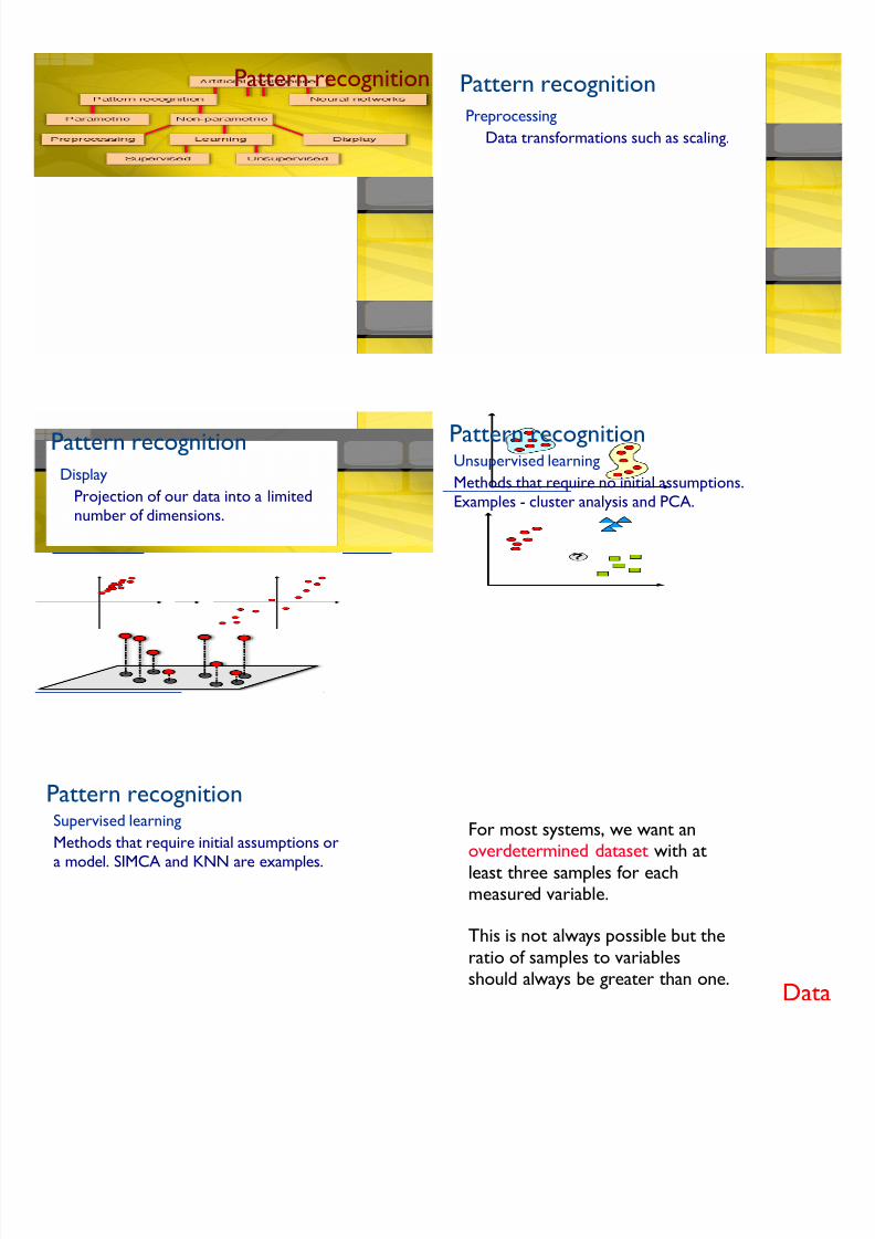
Pattern recognition Pattern recognition

Preprocessing! Data transformations such as scaling.

Pattern recognitionDisplay

Projection of our data into a limited

number of dimensions.

Pattern recognitionUnsupervised learning

Methods that require no initial assumptions.

Examples - cluster analysis and PCA.

Pattern recognitionSupervised learning

Methods that require initial assumptions or

a model. SIMCA and KNN are examples.

Dat

For most systems, we want anoverdetermined dataset with at

least three samples for eachmeasured variable.

This is not always possible but the

ratio of samples to variablesshould always be greater than one.



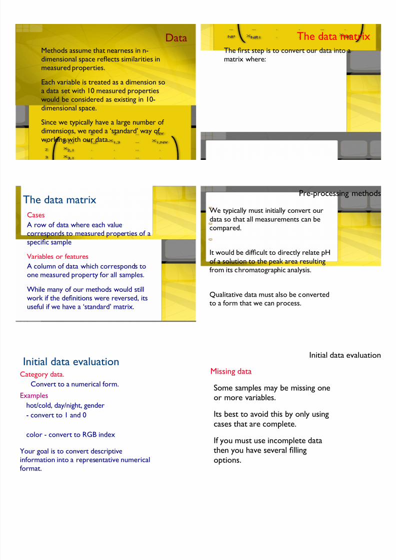
DataMethods assume that nearness in n-

dimensional space reflects similarities in

measured properties.

Each variable is treated as a dimension so

a data set with 10 measured properties

would be considered as existing in 10-dimensional space.

Since we typically have a large number of

dimensions, we need a ‘standard’ way of

working with our data.

The data matrixThe first step is to convert our data into a

matrix where:

The data matrix

Cases

A row of data where each value

corresponds to measured properties of a

specific sample

Variables or features

A column of data which corresponds toone measured property for all samples.

While many of our methods would still

work if the definitions were reversed, its

useful if we have a ‘standard’ matrix.

Pre-processing metho

We typically must initially convert our

data so that all measurements can be

compared.

It would be difficult to directly relate pH

of a solution to the peak area resulting

from its chromatographic analysis.

Qualitative data must also be convertedto a form that we can process.

Initial data evaluationCategory data.

Convert to a numerical form.!

Examples

hot/cold, day/night, gender

- convert to 1 and 0

color - convert to RGB index!

Your goal is to convert descriptive

information into a representative numerical

format.

Initial data evaluat

Missing data

Some samples may be missing oneor more variables.

Its best to avoid this by only using

cases that are complete.

If you must use incomplete datathen you have several filling

options.



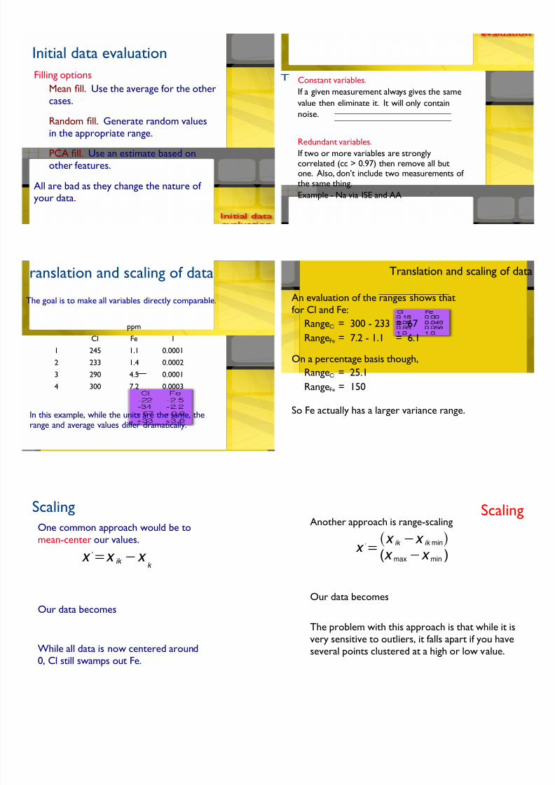
Initial data evaluation

Filling options

Mean fill. Use the average for the other

cases.

Random fill. Generate random values

in the appropriate range.PCA fill. Use an estimate based on

other features.

All are bad as they change the nature of your data.

Constant variables.

If a given measurement always gives the same

value then eliminate it. It will only contain

noise.

Redundant variables.

If two or more variables are stronglycorrelated (cc > 0.97) then remove all butone. Also, don’t include two measurements of the same thing.

Example - Na via ISE and AA

ranslation and scaling of dataThe goal is to make all variables directly comparable.

ppm

Cl Fe I

1 245 1.1 0.0001

2 233 1.4 0.0002

3 290 4.5 0.0001

4 300 7.2 0.0003

In this example, while the units are the same, therange and average values differ dramatically.

Translation and scaling of d

An evaluation of the ranges shows that

for Cl and Fe:! RangeCl = 300 - 233 = 67

! RangeFe = 7.2 - 1.1 = 6.1

On a percentage basis though,! RangeCl = 25.1

! RangeFe = 150

So Fe actually has a larger variance range.

Scaling

One common approach would be to

mean-center our values.

Our data becomes

While all data is now centered around

0, Cl still swamps out Fe.

lx =x ik -x k

ScalingAnother approach is range-scaling

Our data becomes

The problem with this approach is that while it is

very sensitive to outliers, it falls apart if you have

several points clustered at a high or low value.

lx =

(x max-x min )

x ik -x ik min^ h



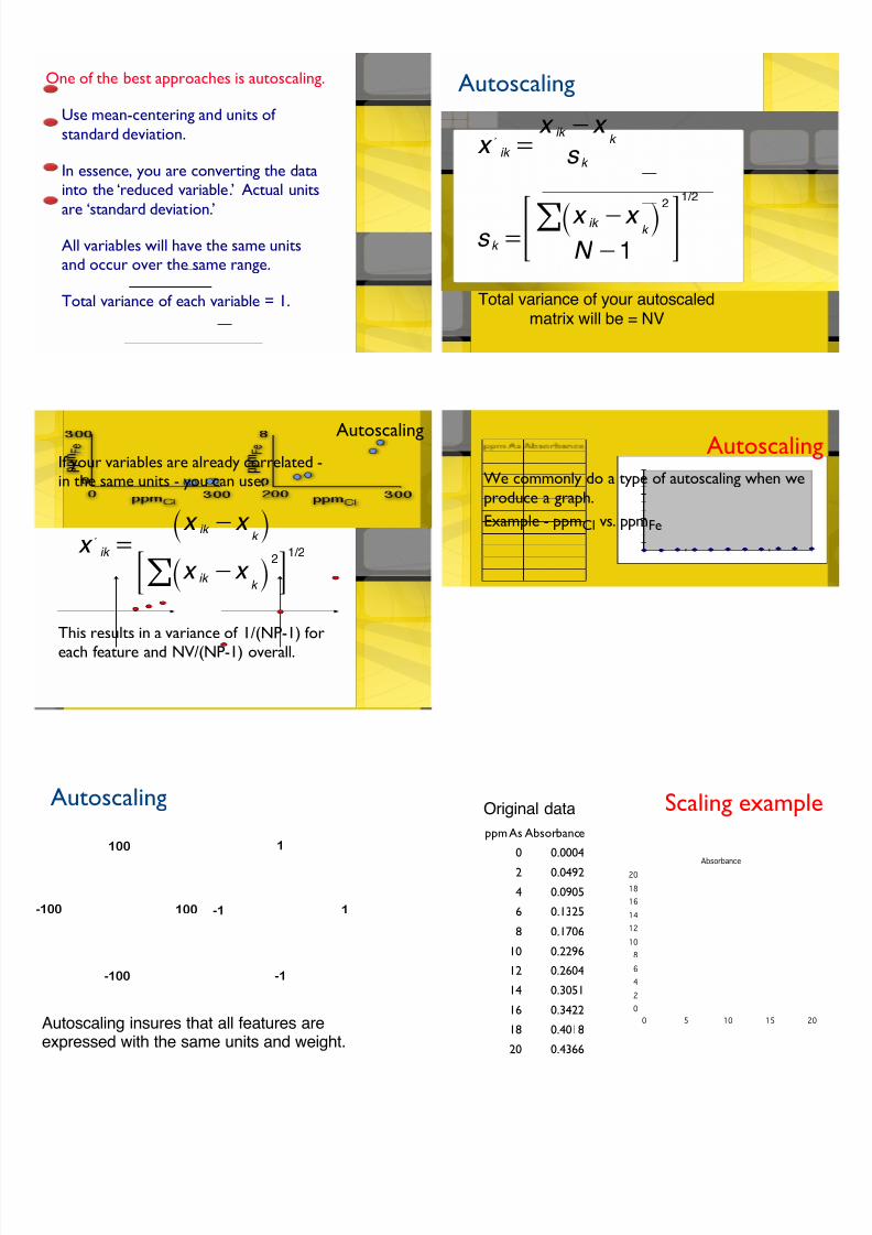
One of the best approaches is autoscaling.

Use mean-centering and units of

standard deviation.

In essence, you are converting the data

into the ‘reduced variable.’ Actual units

are ‘standard deviation.’

All variables will have the same units

and occur over the same range.

Total variance of each variable = 1.

Autoscaling

Total variance of your autoscaledmatrix will be = NV

lx ik = s k

x ik -x k

s k = N -1

x ik -x k ` j!2

> H1/2

AutoscalingIf your variables are already correlated -in the same units - you can use:

This results in a variance of 1/(NP-1) for

each feature and NV/(NP-1) overall.

lx ik =

x ik -x k

` j2

!: D1/2

x ik -x k

` j

Autoscaling

We commonly do a type of autoscaling when we

produce a graph.

Example - ppmCl vs. ppmFe

Autoscaling

Autoscaling insures that all features areexpressed with the same units and weight.

1-1

1

-1

100

-100

100-100

Scaling example

Absorbance

0

2

4

6

8

10

12

14

16

18

20

0 5 10 15 20

Original data

ppm As Absorbance

0 0.0004

2 0.0492

4 0.0905

6 0.1325

8 0.1706

10 0.2296

12 0.2604

14 0.3051

16 0.3422

18 0.4018

20 0.4366



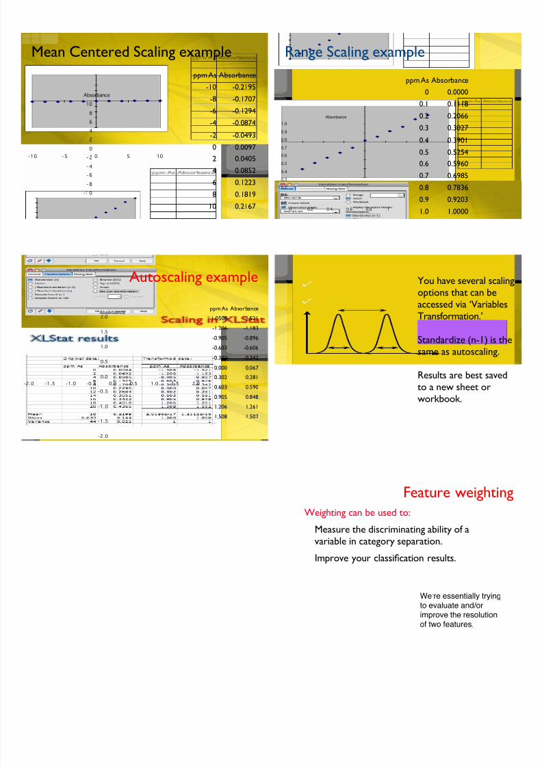
Mean Centered Scaling example

Absorbance

-1 0

- 8

- 6

- 4

- 2

0

2

4

6

8

10

- 10 - 5 0 5 10

ppm As Absorbance

-10 -0.2195

-8 -0.1707

-6 -0.1294

-4 -0.0874

-2 -0.0493

0 0.0097

2 0.0405

4 0.0852

6 0.1223

8 0.1819

10 0.2167

Range Scaling example

Absorbance

0.0

0.1

0.2

0.3

0.4

0.5

0.6

0.7

0.8

0.9

1.0

0 0.2 0.4 0.6 0.8 1

ppm As Absorbance

0 0.0000

0.1 0.1118

0.2 0.2066

0.3 0.3027

0.4 0.3901

0.5 0.5254

0.6 0.5960

0.7 0.6985

0.8 0.7836

0.9 0.9203

1.0 1.0000

Autoscaling example

Absorbance

-2.0

-1.5

-1.0

-0.5

0.0

0.5

1.0

1.5

2.0

-2.0 -1.5 -1.0 -0.5 0.0 0.5 1.0 1.5 2.0

ppm As Absorbance

-1.0508 -1.521

-1.206 -1.183

-0.905 -0.896

-0.603 -0.606

-0.302 -0.342

0.000 0.067

0.302 0.281

0.603 0.590

0.905 0.848

1.206 1.261

1.508 1.502

You have several scalin

options that can be

accessed via ‘Variables

Transformation.’

Standardize (n-1) is th

same as autoscaling.

Results are best saved

to a new sheet or

workbook.

Feature weightin

Weighting can be used to:

Measure the discriminating ability of a

variable in category separation.

Improve your classification results.

Weʼre essentially trying

to evaluate and/or

improve the resolution

of two features.



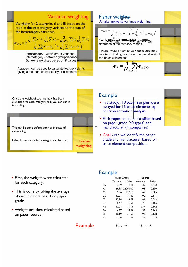
Variance weighting

Weighting for 2 categories (I and II) based on the

ratio of the intercategory variance to the sum of

the intracategory variances.

Approach can be used to calculate feature weights,giving a measure of their ability to discriminate.

w k (I , II )=2

N I

1x I -x I ` j

2

+N II

1x II -x II ` j

2

!!

N I

1x I

2! +N II

1x II

2! -N I N II

2x I

2!N II

1x II

2!

Intracategory - within group variance.Intercategory - between group variance.So, weʼre weighted based on F values.

Fisher weightsAn alternative to variance weighting.

Simply replaced the numerator with thedifference of the category means.

A Fisher weight may actually go to zero for anondiscriminating feature so the overall weightcan be calculated as:

w k (I , II )=

N I

1x I -x

I ` j!

2

+N II

1x II -x

II ` j!

2

x I -x

II

w k =N J

1w k J ] g

J =1

N J

!

Featureweighting

Once the weight of each variable has beencalculated for each category pair, you can use it

for scaling:

This can be done before, after or in place of autoscaling.

Either Fisher or variance weights can be used.

Example

• In a study, 119 paper samples wereassayed for 13 trace elements byneutron activation analysis.

• Each paper could be classified basedon paper grade (40 types) andmanufacturer (9 companies).

• Goal - can we identify the paper

grade and manufacturer based ontrace element composition.

Example

• First, the weights were calculatedfor each category.

• This is done by taking the average

of each element based on papergrade.

• Weights are then calculated based

on paper source.

ExamplePaper Grade Source

Variance Fisher Variance Fisher

Na 7.39 6.62 1.49 0.048

Al 66.95 22240.00 3.03 0.650

Cl 9.96 137.10 1.67 0.085

Ca 13.24 11.08 1.98 0.141

Ti 17.94 12.78 1.66 0.092

Cr 8.67 41.53 1.75 0.106

Mn 13.01 15.53 2.37 0.182

Zn 4.87 18.24 1.99 0.163

Sb 10.19 31.68 1.92 0.138

Ta 2.06 1.71 1.25 0.013

Ngrad

= 40 Nsour

ce

= 9



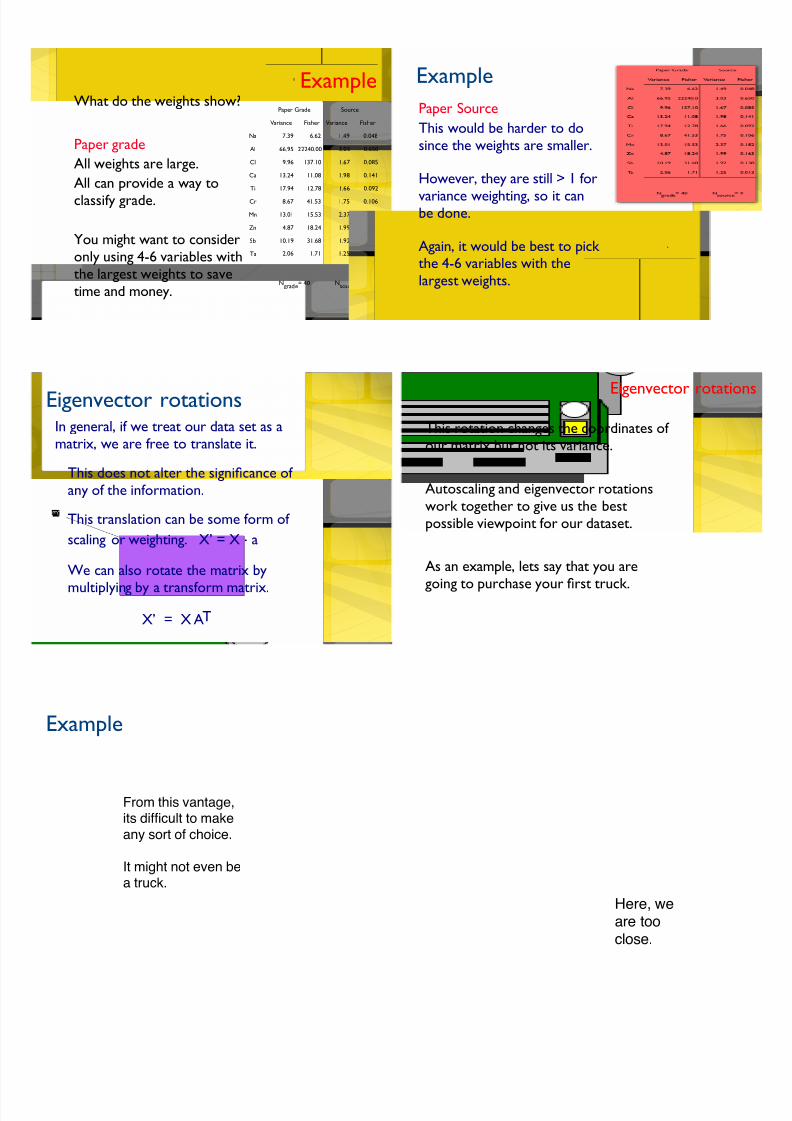
ExampleWhat do the weights show?

Paper grade

All weights are large.

All can provide a way to

classify grade.!You might want to consider

only using 4-6 variables with

the largest weights to save

time and money.

Paper Grade Source

Variance Fisher Variance Fisher

Na 7.39 6.62 1.49 0.048

Al 66.95 22240.00 3.03 0.650

Cl 9.96 137.10 1.67 0.085

Ca 13.24 11.08 1.98 0.141

Ti 17.94 12.78 1.66 0.092

Cr 8.67 41.53 1.75 0.106

Mn 13.01 15.53 2.37 0.182

Zn 4.87 18.24 1.99 0.163

Sb 10.19 31.68 1.92 0.138

Ta 2.06 1.71 1.25 0.013

Ngrad

e= 40 N

sour

ce= 9

Example

Paper Source

This would be harder to do

since the weights are smaller.

However, they are still > 1 for

variance weighting, so it canbe done.

Again, it would be best to pick the 4-6 variables with the

largest weights.

Eigenvector rotationsIn general, if we treat our data set as a

matrix, we are free to translate it.

This does not alter the significance of

any of the information.

This translation can be some form of

scaling or weighting. X’ = X . a

We can also rotate the matrix by

multiplying by a transform matrix.

X’ = X AT

Eigenvector rotatio

This rotation changes the coordinates of

our matrix but not its variance.

Autoscaling and eigenvector rotations

work together to give us the best

possible viewpoint for our dataset.

As an example, lets say that you are

going to purchase your first truck.

Example

From this vantage,its difficult to make

any sort of choice.

It might not even bea truck.

Here, weare tooclose.



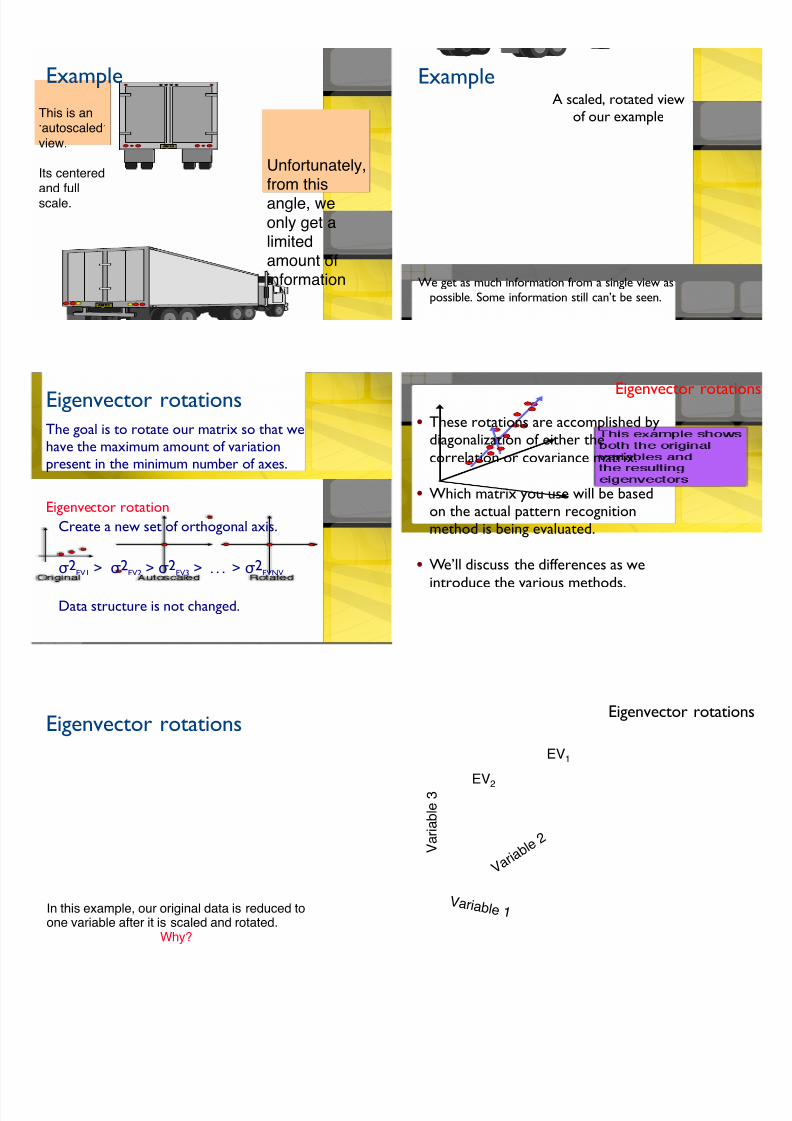
Example

This is an

ʻautoscaledʼ

view.

Its centered

and full

scale.

Unfortunately,

from this

angle, we

only get a

limited

amount of

information

Example

We get as much information from a single view as

possible. Some information still can’t be seen.

A scaled, rotated view

of our example

Eigenvector rotationsThe goal is to rotate our matrix so that we

have the maximum amount of variation

present in the minimum number of axes.

Eigenvector rotation

Create a new set of orthogonal axis.

σ 2EV1 > σ 2EV2 > σ 2EV3 > . . . > σ 2EVNV

! Data structure is not changed.

Eigenvector rotatio

• These rotations are accomplished bydiagonalization of either the

correlation or covariance matrix.

• Which matrix you use will be basedon the actual pattern recognitionmethod is being evaluated.

• We’ll discuss the differences as we

introduce the various methods.

Eigenvector rotations

In this example, our original data is reduced toone variable after it is scaled and rotated.

Why?

Eigenvector rotatio

EV1

EV2

V a r i a b l e 1

V a r i a b l e

2 V a r i a b l e

3



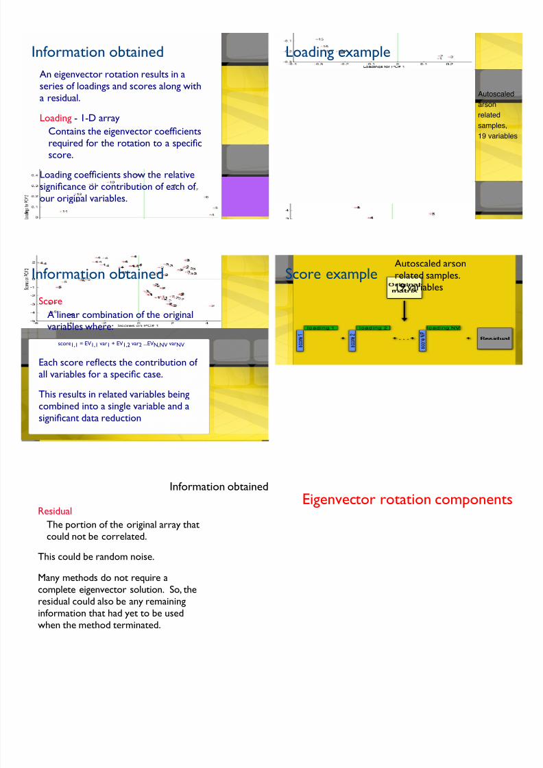
Information obtained

An eigenvector rotation results in a

series of loadings and scores along with

a residual.

Loading - 1-D array

Contains the eigenvector coefficientsrequired for the rotation to a specificscore.

Loading coefficients show the relative

significance or contribution of each of

our original variables.

Loading example

Autoscale

arson

related

samples,

19 variab


Score

A linear combination of the original

variables where:

score1,1 = EV1,1 var1 + EV1,2 var2 ...EVN,NV varNV

Each score reflects the contribution of

all variables for a specific case.

This results in related variables being

combined into a single variable and asignificant data reduction

Score exampleAutoscaled arson

related samples.

19 variables


Residual

The portion of the original array that

could not be correlated.

This could be random noise.

Many methods do not require a

complete eigenvector solution. So, the

residual could also be any remaining

information that had yet to be used

when the method terminated.

Eigenvector rotation components



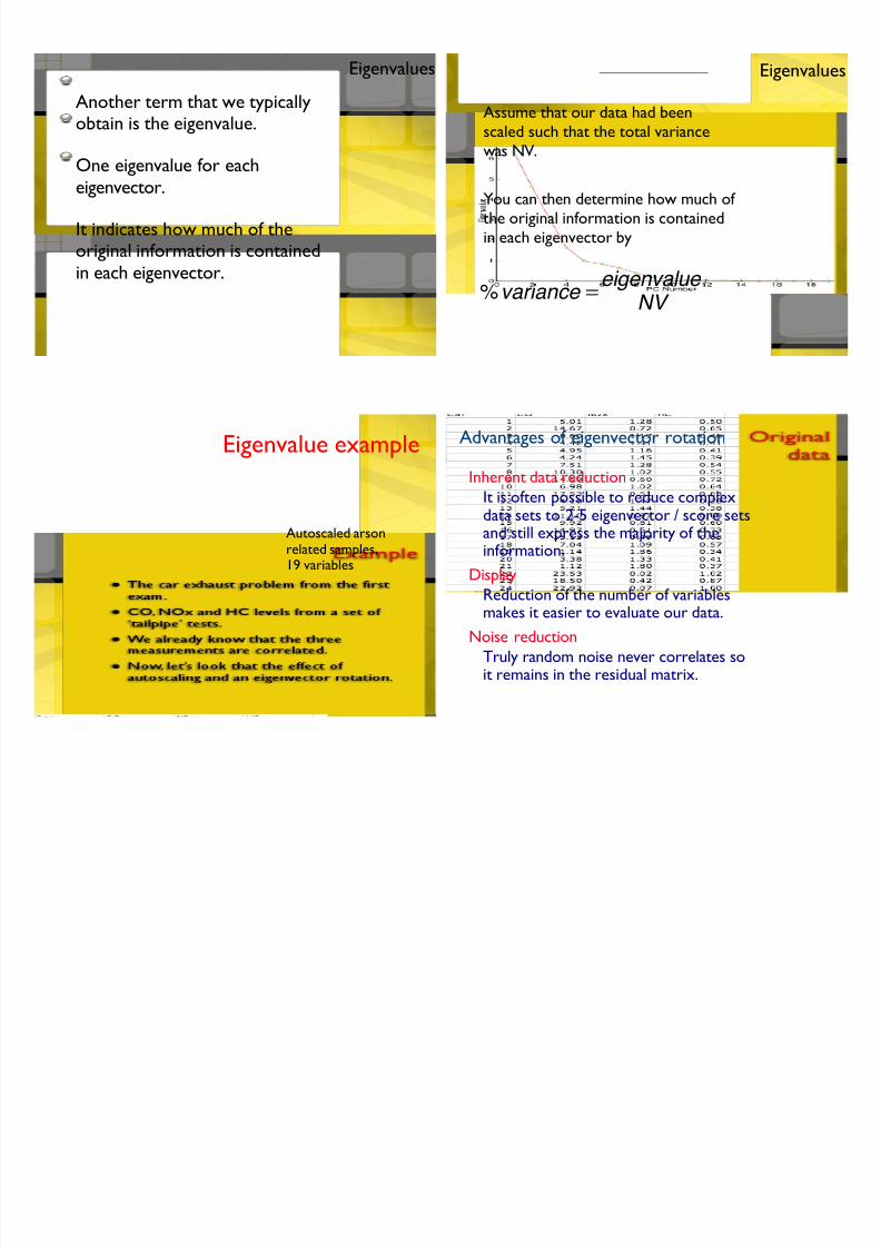
Eigenvalues

Another term that we typicallyobtain is the eigenvalue.

One eigenvalue for each

eigenvector.

It indicates how much of theoriginal information is contained

in each eigenvector.

Eigenvalu

Assume that our data had been

scaled such that the total variance

was NV.

You can then determine how much of

the original information is containedin each eigenvector by

%variance =NV

eigenvalue i

Eigenvalue example

Autoscaled arsonrelated samples,19 variables

Advantages of eigenvector rotation

Inherent data reduction

It is often possible to reduce complexdata sets to 2-5 eigenvector / score setsand still express the majority of theinformation.

Display

Reduction of the number of variablesmakes it easier to evaluate our data.

Noise reduction

Truly random noise never correlates soit remains in the residual matrix.



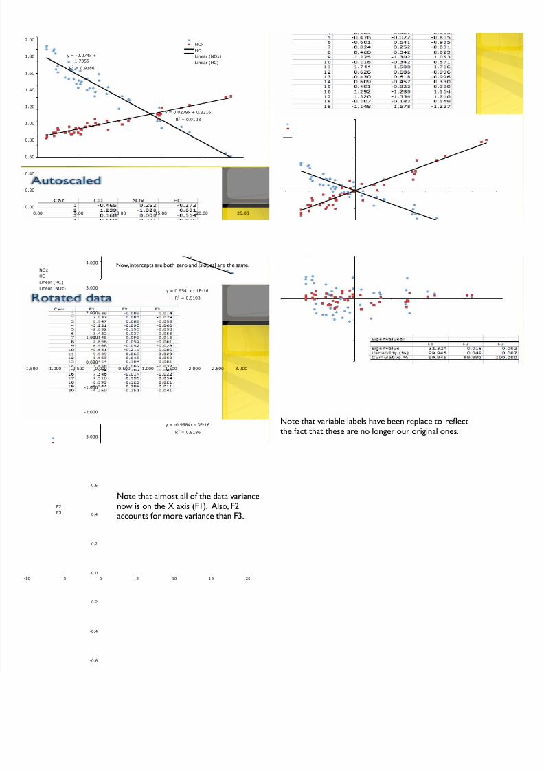
y = -0.074x +

1.7355

R2

= 0.9186

y = 0.0279x + 0.3316

R2

= 0.9103

0.00

0.20

0.40

0.60

0.80

1.00

1.20

1.40

1.60

1.80

2.00

0.00 5.00 10.00 15.00 20.00 25.00

NOx

HC

Linear (NOx)

Linear (HC)

y = 0.9541x - 1E-16

R2

= 0.9103

y = -0.9584x - 3E-16

R2

= 0.9186-3.000

-2.000

-1.000

0.000

1.000

2.000

3.000

4.000

-1.500 -1.000 -0.500 0.000 0.500 1.000 1.500 2.000 2.500 3.000

NOxHC

Linear (HC)

Linear (NOx)

Now, intercepts are both zero and |slopes| are the same.

Note that variable labels have been replace to reflectthe fact that these are no longer our original ones.

-0.6

-0.4

-0.2

0.0

0.2

0.4

0.6

-10 -5 0 5 10 15 20

F2

F3

Note that almost all of the data variancenow is on the X axis (F1). Also, F2accounts for more variance than F3.

Documents

09 Exploration