Embed Size (px)
Citation preview
arX
iv:0
803.
0217
v1 [
cond
-mat
.sta
t-m
ech]
3 M
ar 2
008
Introduction to Monte Carlo
methods for an
Ising Model of a Ferromagnet
‘If God has made the world a perfect mechanism, He
has at least conceded so much to our imperfect intellects
that in order to predict little parts of it, we need not solve
innumerable differential equations, but can use dice with
fair success.’
Max Born
Jacques Kotze

CONTENTS 1
Contents
1 Theory 21.1 Introduction . . . . . . . . . . . . . . . . . . . . . . . . . . . . . . 21.2 Background . . . . . . . . . . . . . . . . . . . . . . . . . . . . . . 21.3 Model . . . . . . . . . . . . . . . . . . . . . . . . . . . . . . . . . 21.4 Computational Problems . . . . . . . . . . . . . . . . . . . . . . . 41.5 Sampling and Averaging . . . . . . . . . . . . . . . . . . . . . . . 51.6 Monte Carlo Method . . . . . . . . . . . . . . . . . . . . . . . . . 81.7 Calculation of observables . . . . . . . . . . . . . . . . . . . . . . 81.8 Metropolis Algorithm . . . . . . . . . . . . . . . . . . . . . . . . 9
2 Results 112.1 Energy Results . . . . . . . . . . . . . . . . . . . . . . . . . . . . 112.2 Magnetization Results . . . . . . . . . . . . . . . . . . . . . . . . 122.3 Exact Results . . . . . . . . . . . . . . . . . . . . . . . . . . . . . 182.4 Finite size scaling . . . . . . . . . . . . . . . . . . . . . . . . . . . 192.5 Conclusion . . . . . . . . . . . . . . . . . . . . . . . . . . . . . . 23
A Monte Carlo source code 26
Acknowledgements
Thank you to Prof B.A. Bassett for encouraging me to submit this report andmy office colleagues in Room 402 for their assistance in reviewing it. A specialthanks must be extended to Dr A.J. van Biljon who was always available forinvaluable discussion, advice and assistance. Dr L. Anton and Dr K. Muller-Nederbok also helped in sharing their expertise with regards this report. LastlyI would like to thank Prof H.B. Geyer for his patience and constructive criticism.
1 THEORY 2
1 Theory
1.1 Introduction
This discussion serves as an introduction to the use of Monte Carlo simulationsas a useful way to evaluate the observables of a ferromagnet. Key backgroundis given about the relevance and effectiveness of this stochastic approach and inparticular the applicability of the Metropolis-Hastings algorithm. Importantlythe potentially devastating effects of spontaneous magnetization are highlightedand a means to avert this is examined.
An Ising model is introduced and used to investigate the properties of atwo dimensional ferromagnet with respect to its magnetization and energy atvarying temperatures. The observables are calculated and a phase transitionat a critical temperature is also illustrated and evaluated. Lastly a finite sizescaling analysis is underatken to determine the critical exponents and the Curietemperature is calculated using a ratio of cumulants with differing lattice sizes.The results obtained from the simulation are compared to exact calculations toendorse the validity of this numerical process. A copy of the code used, writtenin C++, is enclosed and is freely available for use and modification under theGeneral Public License.
1.2 Background
In most ordinary materials the associated magnetic dipoles of the atoms have arandom orientation. In effect this non-specific distribution results in no overallmacroscopic magnetic moment. However in certain cases, such as iron, a mag-netic moment is produced as a result of a preferred alignment of the atomicspins.
This phenomenon is based on two fundamental principles, namely energy
minimization and entropy maximization. These are competing principles andare important in moderating the overall effect. Temperature is the mediatorbetween these opposing elements and ultimately determines which will be moredominant.
The relative importance of the energy minimization and entropy maximiza-tion is governed in nature by a specific probability
P (α) = exp−E(α)
kT. (1)
which is illustrated in Figure 1 and is known as the Gibbs distribution.
1.3 Model
A key ingredient in the understanding of this theory is the spin and associatedmagnetic moment. Knowing that spin is a quantum mechanical phenomenon itis easy to anticipate that a complete and thorough exposition of the problemwould require quantum rules of spin and angular momentum. These factorsprove to be unnecessary complications.
We thus introduce a model to attain useful results. The idea central to amodel is to simplify the complexity of the problem to such a degree that it ismathematically tractable to deal with while retaining the essential physics of

1 THEORY 3
Boltzmann Probability Distrubution vs Energy vs Temprature
0 1 2 3 4 5 6 7 8Energy (E) 0
12
34
56
78
Temprature (T)
00.20.40.60.8
1
Probability
Figure 1: This figure shows the Boltzmann probability distribution as a land-scape for varying Energy (E) and Temperature (T ).
the system. The Ising Model does this very effectively and even allows for agood conceptual understanding.
Figure 2: Two Dimensional lattice illustration of an Ising Model. The up anddown arrows represent a postive and a negative spin respectively.
The Ising Model considers the problem in two dimensions1 and places dipolespins at regular lattice points while restricting their spin axis to be either up(+y) or down (-y). The lattice configuration is square with dimensions L and thetotal number of spins equal to N = L × L. In its simplest form the interactionrange amongst the dipoles is restricted to immediately adjacent sites (nearestneighbours). This produces a Hamiltonian for a specific spin site, i, of the form
Hi = −J∑
jnn
sisj (2)
where the sum jnn runs over the nearest neighbours of i. The coupling constantbetween nearest neighbours is represented by J while the si and sj are the re-spective nearest neighbour spins. The nature of the interaction in the model isall contained in the sign of the interaction coupling constant J . If J is positive
1It may also be considered in three dimensions but it should be noted that a one dimensional
representation does not display phase transition.

1 THEORY 4
it would mean that the material has a ferromagnetic nature (parallel align-ment) while a negative sign would imply that the material is antiferromagentic(favours anti-parallel alignment). J will be taken to be +1 in our discussionand the values for spins will be +1 for spin up and -1 for spin down. A furthersimplification is made in that J/kb is taken to be unity. The relative positioningof nearest neighbours of spins is shown in Figure 3 with the darker dot beinginteracted on by its surrounding neighbours.
J
J
J
J
ABOVE(x ; y+1)
(x+1; y)RIGHTLEFT
(x−1; y)
(x; y−1)BELOW
Figure 3: Nearest neighbour coupling. The dark dot, at position (x,y), is beinginteracted upon by its nearest neighbours which are one lattice spacing awayfrom it.
To maximize the interaction of the spins at the edges of the lattice they aremade to interact with the spins at the geometric opposite edges of the lattice.This is referred to as periodic boundary condition (pbc) and can be visualizedbetter if we consider the 2d lattice being folded into a 3d torus with spins beingon the surface of this topological structure.
Figure 4: An illustration of a three dimensional torus which is repreentative ofa two dimensional lattice with periodic boundary conditions.
1.4 Computational Problems
With the help of an Ising Model we can proceed with the anticipation of achiev-ing solutions for observables. If the energy of each possible state of the system

1 THEORY 5
is specified, then the Boltzmann distribution function, equation (1), gives theprobability for the system to be in each possible state (at a given temperature)and therefore macroscopic quantities of interest can be calculated by doing prob-ability summing. This can be illustrated by using magnetization and energy asexamples. For any fixed state, α, the magnetization is proportional to the ‘ex-cess’ number of spins pointing up or down while the energy is given by theHamiltonian (2).
M(α) = Nup(α) − Ndown(α) (3)
The expected value for M is given by
〈M〉 =∑
α
M(α)P (α), (4)
and the expected value for E is given by
〈E〉 =∑
α
E(α)P (α). (5)
These calculation pose a drastic problem from a practical perspective. Consid-ering we have two spin orientations (up & down) and there are N spins whichimplies that there are 2N different states. As N becomes large it is evident thatcomputations become a daunting task if calculated in this manner.
It may seem a natural suggestion to use a computer simulation to do thesecalculations but by examining equations (4) and (5) more closely it becomesapparent that using this procedure would waste as much computing effort oncalculating an improbable result as it does on a very probable result. Thus abetter numerical alternative would be to use a simulation to generate data overthe ‘representative states’. These representative states constitute the appropri-ate proportions of different states 2. This is a form of biased sampling whichessentially boils down to satisfying the following condition
GENERATED FREQUENCY≡ACTUAL PROBABILITY.(computer) (theory)
We now examine, in a more formal setting, how to accomplish this objective.
1.5 Sampling and Averaging
The thermal average for an observable A(x) is defined in the canonical ensemble
〈A(x)〉T =1
Z
∫
e−βH(x)A(x)dx (6)
where x is a vector in the phase space and β = 1/kbT . The Partition function,Z, is given by
Z =
∫
e−βH(x)dx
while the normalized Boltzmann factor is
2The frequency with which some class of events is encountered in the representative sum
must be the same as the actual probability for that class.
1 THEORY 6
P (x) =1
Ze−βH(x). (7)
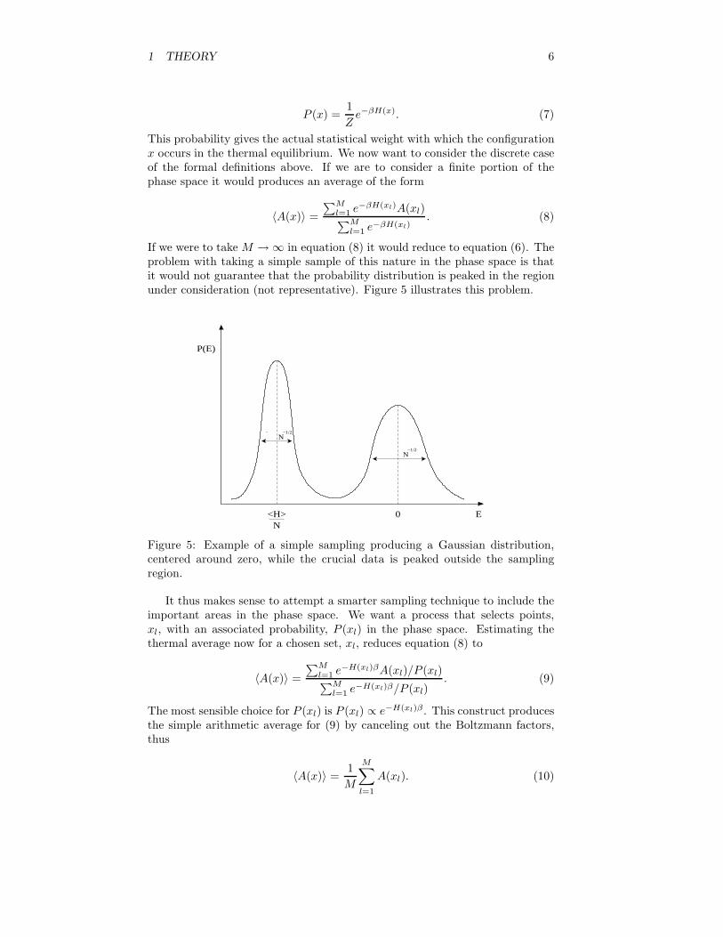
This probability gives the actual statistical weight with which the configurationx occurs in the thermal equilibrium. We now want to consider the discrete caseof the formal definitions above. If we are to consider a finite portion of thephase space it would produces an average of the form
〈A(x)〉 =
∑Ml=1 e−βH(xl)A(xl)∑M
l=1 e−βH(xl). (8)
If we were to take M → ∞ in equation (8) it would reduce to equation (6). Theproblem with taking a simple sample of this nature in the phase space is thatit would not guarantee that the probability distribution is peaked in the regionunder consideration (not representative). Figure 5 illustrates this problem.
−1/2N
−1/2N
0 E
P(E)
<H>N
Figure 5: Example of a simple sampling producing a Gaussian distribution,centered around zero, while the crucial data is peaked outside the samplingregion.
It thus makes sense to attempt a smarter sampling technique to include theimportant areas in the phase space. We want a process that selects points,xl, with an associated probability, P (xl) in the phase space. Estimating thethermal average now for a chosen set, xl, reduces equation (8) to
〈A(x)〉 =
∑Ml=1 e−H(xl)βA(xl)/P (xl)∑M
l=1 e−H(xl)β/P (xl). (9)
The most sensible choice for P (xl) is P (xl) ∝ e−H(xl)β . This construct producesthe simple arithmetic average for (9) by canceling out the Boltzmann factors,thus
〈A(x)〉 =1
M
M∑
l=1
A(xl). (10)
1 THEORY 7
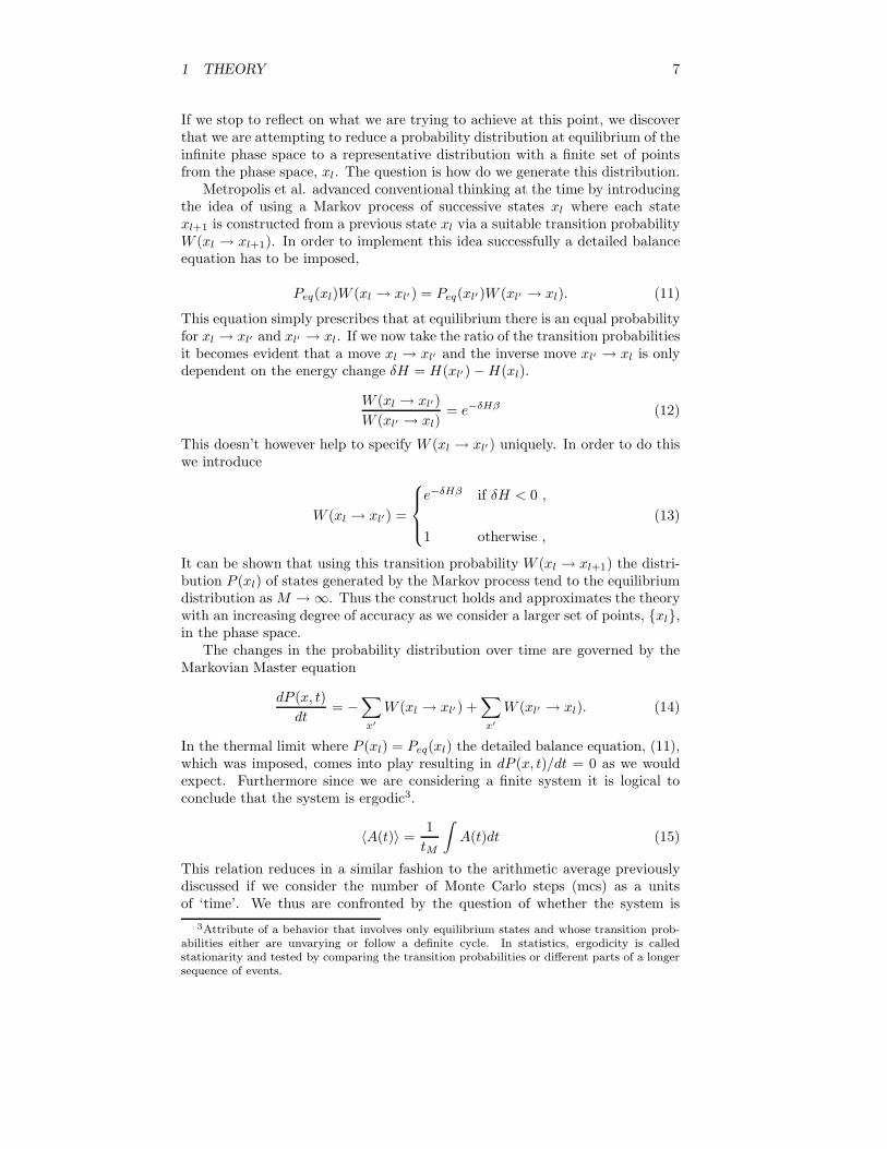
If we stop to reflect on what we are trying to achieve at this point, we discoverthat we are attempting to reduce a probability distribution at equilibrium of theinfinite phase space to a representative distribution with a finite set of pointsfrom the phase space, xl. The question is how do we generate this distribution.
Metropolis et al. advanced conventional thinking at the time by introducingthe idea of using a Markov process of successive states xl where each statexl+1 is constructed from a previous state xl via a suitable transition probabilityW (xl → xl+1). In order to implement this idea successfully a detailed balanceequation has to be imposed,
Peq(xl)W (xl → xl′ ) = Peq(xl′ )W (xl′ → xl). (11)
This equation simply prescribes that at equilibrium there is an equal probabilityfor xl → xl′ and xl′ → xl. If we now take the ratio of the transition probabilitiesit becomes evident that a move xl → xl′ and the inverse move xl′ → xl is onlydependent on the energy change δH = H(xl′) − H(xl).
W (xl → xl′)
W (xl′ → xl)= e−δHβ (12)
This doesn’t however help to specify W (xl → xl′) uniquely. In order to do thiswe introduce
W (xl → xl′) =
e−δHβ if δH < 0 ,
1 otherwise ,
(13)
It can be shown that using this transition probability W (xl → xl+1) the distri-bution P (xl) of states generated by the Markov process tend to the equilibriumdistribution as M → ∞. Thus the construct holds and approximates the theorywith an increasing degree of accuracy as we consider a larger set of points, {xl},in the phase space.
The changes in the probability distribution over time are governed by theMarkovian Master equation
dP (x, t)
dt= −
∑
x′
W (xl → xl′ ) +∑
x′
W (xl′ → xl). (14)
In the thermal limit where P (xl) = Peq(xl) the detailed balance equation, (11),which was imposed, comes into play resulting in dP (x, t)/dt = 0 as we wouldexpect. Furthermore since we are considering a finite system it is logical toconclude that the system is ergodic3.
〈A(t)〉 =1
tM
∫
A(t)dt (15)
This relation reduces in a similar fashion to the arithmetic average previouslydiscussed if we consider the number of Monte Carlo steps (mcs) as a unitsof ‘time’. We thus are confronted by the question of whether the system is
3Attribute of a behavior that involves only equilibrium states and whose transition prob-
abilities either are unvarying or follow a definite cycle. In statistics, ergodicity is called
stationarity and tested by comparing the transition probabilities or different parts of a longer
sequence of events.

1 THEORY 8
ergodic in order for the time averaging to be equivalent to the canonical ensembleaverage. This condition is thus forced upon the system if we consider the mcsas a measure of time.
〈A(t)〉 =1
M
M∑
t=1
A(x(t)) (16)
Thus the Metropolis sampling can be interpreted as time averaging along astochastic trajectory in phase space, controlled by the master equation (14) ofthe system.
1.6 Monte Carlo Method
The fact that we can make a successful stochastic interpretation of the samplingprocedure proves to be pivotal in allowing us to introduce the Monte Carlomethod as a technique to solve for the observables of the Ising Model.
A Monte Carlo calculation is defined, fundamentally, as explicitly using ran-dom variates and a stochastic process is characterized by a random process thatdevelops with time. The Monte Carlo method thus lends itself very naturallyto simulating systems in which stochastic processes occur. From what we haveestablished with regards to the sampling being analogous to a time averagingalong a stochastic trajectory in the phase space it is possible to simulated thisprocess by using the Monte Carlo method. The algorithm used is design aroundthe principle of the Metropolis sampling.
From an implementation point of view the issue of the random number lies atthe heart of this process and its success depends on the fact that the generatednumber is truly random. ‘Numerical Recipes in C’, [9], deals with this issueextensively and the random number generator ‘Ran1.c’ from this text was usedin the proceeding simulation. This association with randomness is also the originof the name of the simulation since the glamorous location of Monte Carlo issynonymous with luck and chance.
1.7 Calculation of observables
The observables of particular interest are 〈E〉, 〈E2〉, 〈M〉, 〈|M |〉 and 〈M2〉.These are calculated in the following way,
〈M〉 =1
N
N∑
α
M(α) (17)
similarly 〈|M |〉 and 〈M2〉 are calculated using the above equation.To calculate energy we use the Hamiltonian given in equation (2),
〈E〉 =1
2〈
N∑
i
Hi 〉 =1
2〈 −J
N∑
i
∑
jnn
sisj 〉 (18)
the factor of a half is introduced in order to account for the spins being countedtwice. Equation (18) is used in a similar way to determine 〈E2〉.
At the Curie temperature we expect a marked fluctuation in these quan-tities. A good candidate to illustrate this fluctuation would be the variance
1 THEORY 9
(∆A)2 = 〈A2〉− 〈A〉2. This leads us to the logical conclusion of calculating theheat capacity, C, and the susceptibility, χ.
C =∂E
∂T=
(∆E)2
kbT=
〈E2〉 − 〈E〉2
kbT 2(19)
χ =∂M
∂T=
(∆M)2
kbT=
〈M2〉 − 〈M〉2
kbT(20)
A cumulant is also calculated. This will be used to ultimately determine theCurie temperature.
UL = 1 −〈M4〉L3〈M2〉L
(21)
1.8 Metropolis Algorithm
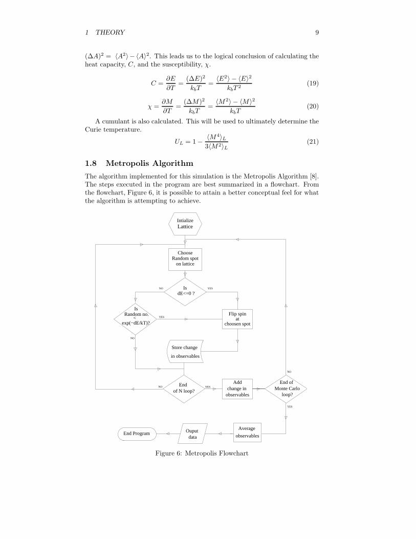
The algorithm implemented for this simulation is the Metropolis Algorithm [8].The steps executed in the program are best summarized in a flowchart. Fromthe flowchart, Figure 6, it is possible to attain a better conceptual feel for whatthe algorithm is attempting to achieve.
Choose
on latticeRandom spot
at
Average
observables
in observables
Store change
Add
observableschange in
dataOuput End Program
Lattice
YES
NO
NO YES
NO
YES
Intialize
Is
< Random no.
exp(−dE/kT)?
dE<=0 ?Is
Flip spin
choosen spot
YES
loop?Monte Carlo
End of
of N loop?EndNO
Figure 6: Metropolis Flowchart
1 THEORY 10
• In the first step the lattice is INITIALIZED to a starting configuration.This may either be a homogeneous or random configuration. A randomconfiguration has a benefit in that it uses less computing time to reach aequilibrated configuration with the associated heat bath.
• In the following PROCESS the random number generator is used to se-lect a position on the lattice by producing a uniformly generated numberbetween 1 and N .
• A DECISION is then made whether the change in energy of flipping thatparticular spin selected is lower than zero. This is in accordance with theprinciple of energy minimization.
– If the change in energy is lower than zero then a PROCESS is invokedto flip the spin at the selected site and the associated change in theobservables that want to be monitored are stored.
– If the change in energy is higher than zero then a DECISION has tobe used to establish if the spin is going to be flipped, regardless of thehigher energy consideration. A random number is generated between0 and 1 and then weighed against the Boltzmann Probability factor.If the random number is less than the associated probability, e−δβH ,then the spin is flipped (This would allow for the spin to be flippedas a result of energy absorbed from the heat bath, as in keeping withthe principle of entropy maximization) else it is left unchanged in itsoriginal configuration.
• The above steps are repeated N times and checked at this point in aDECISION to determine if the loop is completed. The steps referred tohere do not include the initialization which is only required once in thebeginning of the algorithm.
• Once the N steps are completed a PROCESS is used to add all the pro-gressive changes in the lattice configuration together with the originalconfiguration in order to produce a new lattice configuration.
• All these steps are, in turn, contained within a Monte Carlo loop. ADECISION is used to see if these steps are completed.
• Once the Monte Carlo loop is completed the program is left with, whatamounts to, the sum of all the generated lattices within the N loops. APROCESS is thus employed to average the accumulated change in observ-ables over the number of spins and the number of Monte Carlo steps.
• Lastly this data can be OUTPUT to a file or plot.
This run through the algorithm produces a set of observables for a specifictemperature. Considering that we are interested in seeing a phase transitionwith respect to temperature we need to contain this procedure within a temper-ature loop in order to produce these observables for a range of temperatures.
The program that was implemented for this discussion started at a temper-ature of T = 5 and progressively stepped down in temperature to T = 0.5 withintervals of δT = 0.1. The different lattice sizes considered where 2 × 2, 4 × 4,
2 RESULTS 11
8 × 8 and 16 × 16. A million Monte Carlo steps (mcs) per spin where used inorder to ensure a large sample of data to average over. The physical variablescalculated were 〈E〉, 〈E2〉, 〈|M |〉 and 〈M2〉.
A problem that occurs after the initialization is that the configuration will,more than likely, not be in equilibrium with the heat bath and it will take a fewMonte Carlo steps to reach a equilibrated state. The results produced duringthis period are called transient and aren’t of interest. We thus have to makeprovision for the program to disregard them. This is achieved by doing a run ofa thousand Monte Carlo steps preceding the data collection of any statistics fora given temperature in order to ensure that it has reached a equilibrated state.This realization is only significant for the initial configuration and the problem isavoided by the program in the future by using small temperature steps and theconfiguration of the lattice at the previous temperature. A very small numberof mcs are thus required for the system to stabilize its configuration to the newtemperature.
2 Results
2.1 Energy Results
-2
-1.8
-1.6
-1.4
-1.2
-1
-0.8
-0.6
-0.4
0.5 1 1.5 2 2.5 3 3.5 4 4.5 5
Ene
rgy
per
spin
(E
/N)
Temperature (T)
Energy per spin (E/N) vs Temperature (T)
L=2L=4L=8
L=16
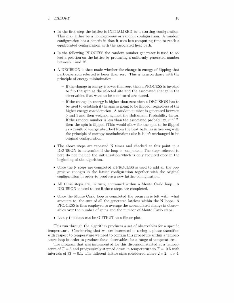
Figure 7: This plot shows the differing results of the Energy for varying latticesizes, L × L.
In Figure 7 the energy per spin as a function of temperature can be seen.The curve of the graph becomes more pronounced as the lattice size increasesbut there isn’t a marked difference between the L = 8 and L = 16 lattices. Thesteep gradient in the larger lattices points towards a possible phase transitionbut isn’t clearly illustrated. The energy per spin for higher temperatures isrelatively high which is in keeping with our expectation of having a randomconfiguration while it stabilizes to a E/N = −2J = −2 at low temperatures.This indicates that the spins are all aligned in parallel.

2 RESULTS 12
0
0.2
0.4
0.6
0.8
1
1.2
1.4
1.6
0.5 1 1.5 2 2.5 3 3.5 4 4.5 5
Hea
t Cap
acity
per
spi
n (C
/N)
Temperature (T)
Specific Heat Capacity per spin (C/N) vs Temperature (T)
L=2L=4L=8
L=16
Figure 8: This plot shows the differing results of Specific Heat Capacity forvarying lattice sizes, L × L.
In Figure 8 the specific heat capacity per spin is shown as a function of tem-perature. We concluded previously that a divergence would occur at a phasetransition and thus should be looking for such a divergence on the graph. It ishowever clear that there is no such divergence but merely a progressive steep-ening of the peak as the lattice size increases. The point at which the plot ispeaked should be noted as a possible point of divergence. The reason for notexplicitly finding a divergence will be discussed in Section 2.4.
2.2 Magnetization Results
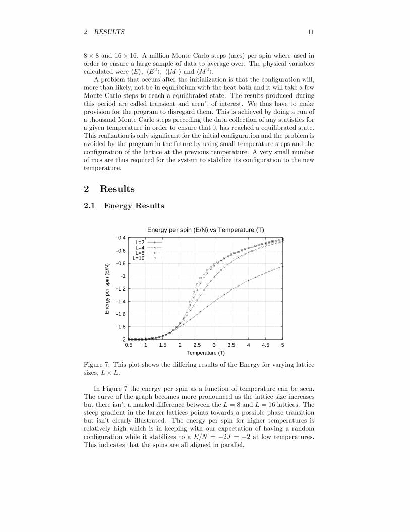
Figure 9 of the magnetization results shows very beautifully that the shapeof the gradient becomes more distinct as the lattice size is increased. Fur-thermore, as opposed to Figure 7, there is a far more apparent difference thatthe larger lattices produce in the curves and this illustrates a more apparentcontinuous phase transition. The behaviour of the magnetization at high andlow temperature are as the theory prescribes (random to stable parallel alignedconfiguration).
At this juncture it is prudent to point out that the susceptibility cannot becalculated using the ordinary technique in equation (20) given in the discussionon the calculation of observables. The reason is focused around a subtle factthat has drastic implications. To comprehend the problem at work we have toconsider one of the constraints of our model, namely the finite nature of ourlattice. This manifests in the fact that spontaneous magnetization can occurfor a finite sized lattice. In this instance the effect is of particular interest belowthe critical temperature.
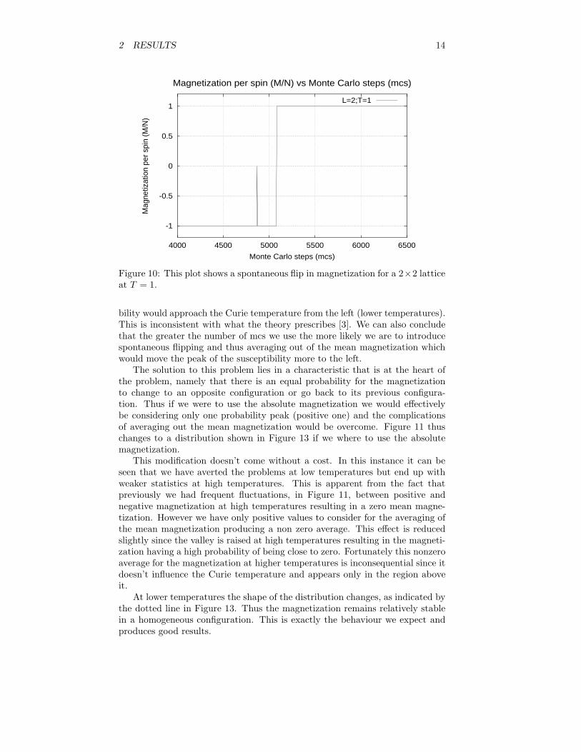
This can be illustrated by considering the following example of collecteddata in Figure 10. This data is taken at a temperature that is considerablyless than the Curie temperature and we would thus expect it to have a stablenature and yet it clearly displays a fluctuation that is uncharacteristic, resulting
2 RESULTS 13
0
0.1
0.2
0.3
0.4
0.5
0.6
0.7
0.8
0.9
1
0.5 1 1.5 2 2.5 3 3.5 4 4.5 5
Abs
olut
e M
agne
tisat
ion
(<|M
|>/N
)
Temperature (T)
Absolute Magnetisation per spin (<|M|>/N) vs Temperature (T)
L=2L=4L=8
L=16
Figure 9: This plot shows the differing results of the Magnetization for varyinglattice sizes, L × L.
in a complete flip of the magnetization. It has already been highlighted thatbecause we are dealing with a limited lattice size there is finite probability forthis kind of behaviour to take place. This probability is directly proportionalto the number of mcs used and inversely proportional to the lattice size, this iscompounded by the preiodic boundary conditions used.
Figure 11 schematically depicts this fact. The valley shown linking the twopeaks of the probability will thus be dropped for lower temperatures and biggerlattice configurations. It should be noted that even though the probability maybe less it does always exist and this has to be accounted for in data collection orit may corrupt the results. We expect the configuration to be relatively stableat the peaks but if its magnetization has slipped down (fluctuated) to the centerof the valley then it has an equal probability of climbing up either side of thepeaks, this is the crux of the spontaneous flipping. This aspect of symmetryproves to also be the seed for a possible solution to this problem.
As an example of what has just been mentioned we note from Figure 10where a fluctuation occurs just before 5000 mcs and the magnetization peaksat 0 from −1. The configuration is now in the middle of the valley and happensto go back to its previous state. The same phenomenon occurs just after 5000mcs but in this instance chooses to flip to an opposite, but equally probable,magnetization, from -1 to 1.
If we now were to think of the implications of this spontaneous flippingwe come to the realization that it would cause an averaging out of the meanmagnetization, 〈M〉. This of course has a detrimental effect on calculating thevariance of the magnetization and thus the susceptibility.
This can be illustrated in the Figure 12 where the plot shows that 〈M〉2
remains zero for an extended period at low temperatures. This would causethe variance to peak at lower temperatures. As the lattice size increases thespontaneous magnetization is less likely to occur and the critical point movesprogressively to higher temperatures, this implies that the peak for the suscepti-
2 RESULTS 14
-1
-0.5
0
0.5
1
4000 4500 5000 5500 6000 6500
Mag
netiz
atio
n pe
r sp
in (
M/N
)
Monte Carlo steps (mcs)
Magnetization per spin (M/N) vs Monte Carlo steps (mcs)
L=2;T=1
Figure 10: This plot shows a spontaneous flip in magnetization for a 2×2 latticeat T = 1.
bility would approach the Curie temperature from the left (lower temperatures).This is inconsistent with what the theory prescribes [3]. We can also concludethat the greater the number of mcs we use the more likely we are to introducespontaneous flipping and thus averaging out of the mean magnetization whichwould move the peak of the susceptibility more to the left.
The solution to this problem lies in a characteristic that is at the heart ofthe problem, namely that there is an equal probability for the magnetizationto change to an opposite configuration or go back to its previous configura-tion. Thus if we were to use the absolute magnetization we would effectivelybe considering only one probability peak (positive one) and the complicationsof averaging out the mean magnetization would be overcome. Figure 11 thuschanges to a distribution shown in Figure 13 if we where to use the absolutemagnetization.
This modification doesn’t come without a cost. In this instance it can beseen that we have averted the problems at low temperatures but end up withweaker statistics at high temperatures. This is apparent from the fact thatpreviously we had frequent fluctuations, in Figure 11, between positive andnegative magnetization at high temperatures resulting in a zero mean magne-tization. However we have only positive values to consider for the averaging ofthe mean magnetization producing a non zero average. This effect is reducedslightly since the valley is raised at high temperatures resulting in the magneti-zation having a high probability of being close to zero. Fortunately this nonzeroaverage for the magnetization at higher temperatures is inconsequential since itdoesn’t influence the Curie temperature and appears only in the region aboveit.
At lower temperatures the shape of the distribution changes, as indicated bythe dotted line in Figure 13. Thus the magnetization remains relatively stablein a homogeneous configuration. This is exactly the behaviour we expect andproduces good results.

2 RESULTS 15
L
0 +|Msp|−|Msp|
P(M)
Figure 11: A schematic illustration of the probability density of the magneti-zation and how the representative spin distribution would populate a squarelatice of size L. The darker and lighter regions depict negative and positive spinrepsectively.
The susceptibility that is produced in our data is thus not exactly equivalentto the theoretical susceptibility, χ, and we will be distinguished as χ′. The scal-ing characteristic of this susceptibility is, however, equivalent to the theoreticalvalue and only varies by a constant factor above the Curie temperature.
χ′ =〈M2〉 − 〈|M |〉2
kbT(22)
A comparison can be made between χ′ and χ in Figures 14 and 15 respec-tively. It is clear that a marked difference in results occurs. This mistakebecomes even more evident if you were to use χ to get the critical exponentusing finite size scaling. Only χ′ produces the correct finite size scaling.
We now evaluate the plots produced using this technique discussed thus far.The more distinctive character of the differing plots of Figure 9 produce moredramatic peaks in Figure 14 of the magnetic susceptibility (χ′) per spin versustemperature as a result. This, once again, doesn’t show an exact divergencebut shows a sharp peak for the L = 16 lattice. This should be strong evidenceeluding to a second order phase transition.

2 RESULTS 16
0
0.1
0.2
0.3
0.4
0.5
0.6
0.7
0.8
0.9
1
0.5 1 1.5 2 2.5 3 3.5 4 4.5 5
< M
>2 ; <
|M|>
2 and
< M
2 >
Temperature (T)
< M >2; <|M|>2 and < M2 > vs Temperature (T), L(2)
<|M|>2
< M >2
< M2 >
0
0.1
0.2
0.3
0.4
0.5
0.6
0.7
0.8
0.9
1
0.5 1 1.5 2 2.5 3 3.5 4 4.5 5
< M
>2 ; <
|M|>
2 and
< M
2 >
Temperature (T)
< M >2; <|M|>2 and < M2 > vs Temperature (T), L(4)
<|M|>2
< M >2
< M2 >
0
0.1
0.2
0.3
0.4
0.5
0.6
0.7
0.8
0.9
1
0.5 1 1.5 2 2.5 3 3.5 4 4.5 5
< M
>2 ; <
|M|>
2 and
< M
2 >
Temperature (T)
< M >2; <|M|>2 and < M2 > vs Temperature (T), L(8)
<|M|>2
< M >2
< M2 >
0
0.1
0.2
0.3
0.4
0.5
0.6
0.7
0.8
0.9
1
0.5 1 1.5 2 2.5 3 3.5 4 4.5 5
< M
>2 ; <
|M|>
2 and
< M
2 >
Temperature (T)
< M >2; <|M|>2 and < M2 > vs Temperature (T), L(16)
<|M|>2
< M >2
< M2 >
Figure 12: This is an illustration of the differences in the normalized values of〈M〉2; 〈|M |〉2 and 〈M2〉 with respect to temperature. The varying lattice sizesconsiderd are 2x2 (top left); 4x4 top right; 8x8 (bottom left) and 16x16 (bottomright).
0
P(M)
+|Msp|
Figure 13: The solid line shows the revised probability density when usingthe absolute magnetization as opposed to the dotted line which represents theorginal propability density for magnetization.

2 RESULTS 17
0
1
2
3
4
5
6
7
0.5 1 1.5 2 2.5 3 3.5 4 4.5 5
Mag
netic
Sus
cept
abili
ty p
er s
pin
(X/N
)
Temperature (T)
Magnetic Susceptability per spin (X/N) vs Temperature (T)
L=2L=4L=8
L=16
Figure 14: This plot shows the differing results of the susceptibility for varyinglattice sizes, L × L.
0
10
20
30
40
50
60
70
80
90
100
0.5 1 1.5 2 2.5 3 3.5 4 4.5 5
Mag
netic
Sus
cept
abili
ty p
er s
pin
(X/N
)
Temperature (T)
Magnetic Susceptability per spin (X/N) vs Temperature (T)
L=2L=4L=8
L=16
Figure 15: This plot shows the differing results of the susceptibility for varyinglattice sizes, L × L.

2 RESULTS 18
2.3 Exact Results
As pointed out in the beginning of this work there are significant challenges tothe calculation of exact solutions but we do need to evaluate the dependabilityof the numerical process used in this discussion. For this purpose we restrictthe comparison between simulation and exact results to only a 2 × 2 This onlyserves as a good first order approximation but the corroboartion should imporveas the lattice size is increased.
The 24 different configurations that can be listed can be reduced by sym-metric considerations to only four configurations. Configuration A is the fully
C
A B
D
Figure 16: The four significant lattice configurations for a 2 × 2 lattice.
aligned spin configuration and configuration B has one spin in the opposite di-rection to the other three while C and D have two spins up and two spins down.To generate the full sixteen different configurations we need only consider geo-metric variations of these four configurations.
Using equations (18) and (17) we can calculate the energy and magnetizationfor each of the four configurations. Taking into account the degeneracy of eachof these configurations allows us to generate the exact equations for calculatingthe relevant observables. These results are listed in Table 1.
Configuration Degeneracy Energy(E) Magnetization(M)A 2 -8 +4,-4B 8 0 +2,-2C 4 0 0D 2 8 0
Table 1: Energy and Magnetization for respective configurations illustrated inFigure 16.
Using equations (4) and (5) in conjunction with the results of Table 1 pro-duces the following equations

2 RESULTS 19
Z = 2 e8βJ + 12 + 2 e−8β (23)
〈E〉 = −1
Z[ 2(8) e8β + 2(−8) e−8β ] (24)
〈E2〉 =1
Z[ 2(64) e8β + 2(64) e−8β ] (25)
〈|M |〉 =1
Z[ 2(4) e8β + 8(2) ] (26)
〈M2〉 =1
Z[ 2(16) e8β + 8(4) ]. (27)
Applying equations (24); (25); (26) and (27) to the formulas given in (19)and (22) we can obtain the heat capacity and susceptibility respectively. Thecomparison of these results are shown in Figure 17. The results achieved by theMonte Carlo method match the exact calculation exceptionally well and onlydeviate very slightly from the prescribed heat capacity at high temperatures.
0
0.02
0.04
0.06
0.08
0.1
0.12
0.14
0.16
0.5 1 1.5 2 2.5 3 3.5 4 4.5 5
Sus
cept
ibili
ty p
er s
pin
(X’/N
)
Temperature (T)
Susceptibility per spin (X’/N) vs Temperature (T)
ExactMonte Carlo
0
0.05
0.1
0.15
0.2
0.25
0.3
0.35
0.4
0.45
0.5 1 1.5 2 2.5 3 3.5 4 4.5 5
Spe
cific
Hea
t Cap
acity
per
spi
n (C
/N)
Temperature (T)
Specific Heat Capacity per spin (C/N) vs Temperature (T)
ExactMonte Carlo
Figure 17: This plot shows a favourable comparison between the exact calcula-tions done for the Heat Capacity per spin (C/N) and the Susceptibility per spin(χ′/N) with the numerically generated solutions of the Monte Carlo simulation.
2.4 Finite size scaling
One of the limitations that the Ising Model confronts us with is the finite size ofour lattice. This results in a problem of recognizing the specific point at whichthe phase transition occurs. This should be at a theoretical point of divergencebut we are limited by the size of the lattice under consideration and thus dont seethis divergence. This effect is minimized by using periodic boundary conditionsbut would only be resolved if we where to consider an infinitely sized latticeas with the associated theoretical values for the phase transition. It is thusnecessary to use a construct that will allow us to extrapolate the respectivetheoretical value given the limited resource of a finite sized lattice. The aptlynamed procedure of finite size scaling is used to do just this.
It becomes useful to define a critical exponent to better understand thenature of the divergence near the critical temperature. The critical exponent,
λ, is given by λ = limt→0ln |F (t)|
ln |t| or more commonly written as F (t) ∼ |t|λ
where t = (T − Tc). This exponent is important in the sense that it offers amore universal characteristic for differing data collected. This attribute will be
2 RESULTS 20
taken advantage of and illustrated by showing that in a reduced unit plot thedata collapses to a common curve with the same critical exponent.
The critical exponents relevant to the Ising model are as follows:
ξ(T ) ∼ |T − Tc|−ν
M(T ) ∼ (Tc − T )β
C ∼ |T − Tc|−α
χ ∼ |T − Tc|−γ
If we examine the relationship between the lattice size, L, with respect to thetemperature relationship, |T − Tc|, we discover that |T − Tc| << 1 as L → ∞.Thus a critical exponent is also applicable for the lattice size. This producesL ∼ |Tc(L = ∞) − Tc(L)|−ν which can in turn be used to reduce the aboveexponents for the Ising model to a more appropriate form, in terms of latticesize.
ξ(T ) ∼ |T − Tc|−ν → L (28)
M(T ) ∼ (Tc − T )β → L−β/ν (29)
C(T ) ∼ |T − Tc|−α → Lα/ν (30)
χ ∼ |T − Tc|−γ → Lγ/ν (31)
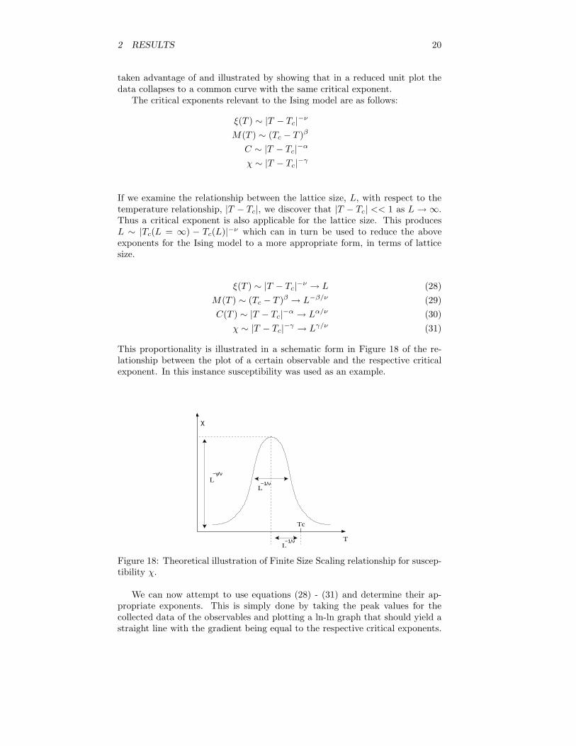
This proportionality is illustrated in a schematic form in Figure 18 of the re-lationship between the plot of a certain observable and the respective criticalexponent. In this instance susceptibility was used as an example.
−1/ν
L
Tc
T
χ
−γ/ν
L
−1/νL
Figure 18: Theoretical illustration of Finite Size Scaling relationship for suscep-tibility χ.
We can now attempt to use equations (28) - (31) and determine their ap-propriate exponents. This is simply done by taking the peak values for thecollected data of the observables and plotting a ln-ln graph that should yield astraight line with the gradient being equal to the respective critical exponents.
2 RESULTS 21
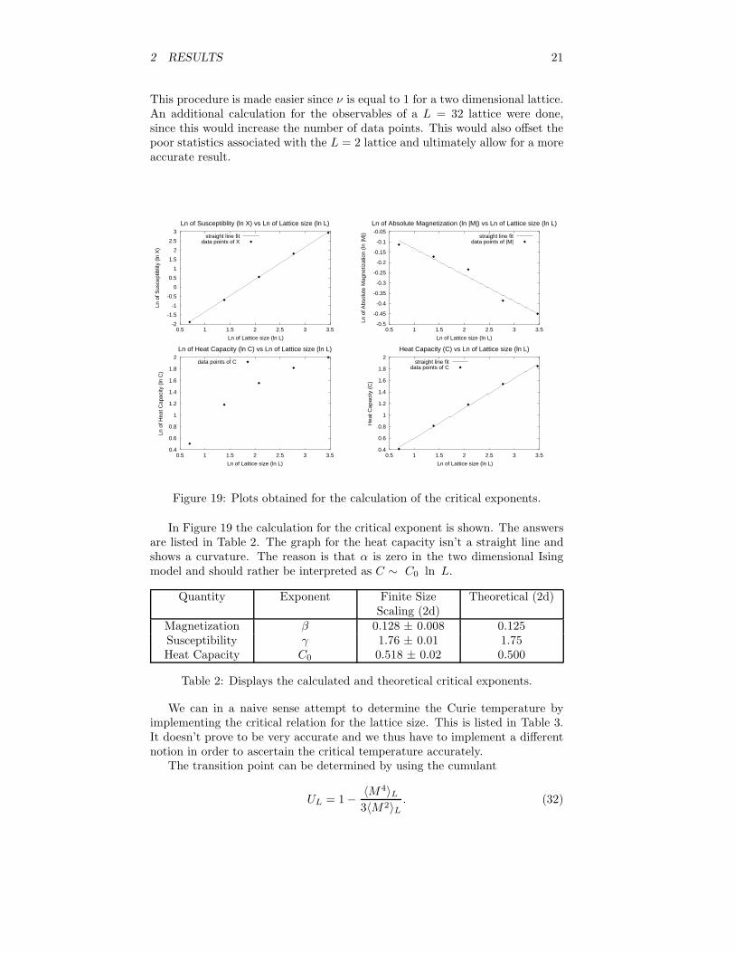
This procedure is made easier since ν is equal to 1 for a two dimensional lattice.An additional calculation for the observables of a L = 32 lattice were done,since this would increase the number of data points. This would also offset thepoor statistics associated with the L = 2 lattice and ultimately allow for a moreaccurate result.
-2
-1.5
-1
-0.5
0
0.5
1
1.5
2
2.5
3
0.5 1 1.5 2 2.5 3 3.5
Ln o
f Sus
cept
iblit
y (ln
X)
Ln of Lattice size (ln L)
Ln of Susceptiblity (ln X) vs Ln of Lattice size (ln L)
straight line fitdata points of X
0.4
0.6
0.8
1
1.2
1.4
1.6
1.8
2
0.5 1 1.5 2 2.5 3 3.5
Hea
t Cap
acity
(C
)
Ln of Lattice size (ln L)
Heat Capacity (C) vs Ln of Lattice size (ln L)
straight line fitdata points of C
-0.5
-0.45
-0.4
-0.35
-0.3
-0.25
-0.2
-0.15
-0.1
-0.05
0.5 1 1.5 2 2.5 3 3.5
Ln o
f Abs
olut
e M
agne
tizat
ion
(ln |M
|)
Ln of Lattice size (ln L)
Ln of Absolute Magnetization (ln |M|) vs Ln of Lattice size (ln L)
straight line fitdata points of |M|
0.4
0.6
0.8
1
1.2
1.4
1.6
1.8
2
0.5 1 1.5 2 2.5 3 3.5
Ln o
f Hea
t Cap
acity
(ln
C)
Ln of Lattice size (ln L)
Ln of Heat Capacity (ln C) vs Ln of Lattice size (ln L)
data points of C
Figure 19: Plots obtained for the calculation of the critical exponents.
In Figure 19 the calculation for the critical exponent is shown. The answersare listed in Table 2. The graph for the heat capacity isn’t a straight line andshows a curvature. The reason is that α is zero in the two dimensional Isingmodel and should rather be interpreted as C ∼ C0 ln L.
Quantity Exponent Finite SizeScaling (2d)
Theoretical (2d)
Magnetization β 0.128 ± 0.008 0.125Susceptibility γ 1.76 ± 0.01 1.75Heat Capacity C0 0.518 ± 0.02 0.500
Table 2: Displays the calculated and theoretical critical exponents.
We can in a naive sense attempt to determine the Curie temperature byimplementing the critical relation for the lattice size. This is listed in Table 3.It doesn’t prove to be very accurate and we thus have to implement a differentnotion in order to ascertain the critical temperature accurately.
The transition point can be determined by using the cumulant
UL = 1 −〈M4〉L3〈M2〉L
. (32)

2 RESULTS 22
-0.01
0
0.01
0.02
0.03
0.04
0.05
-30 -20 -10 0 10 20 30 40
Ln o
f Hea
t Cap
acity
(ln
C)
Ln of Lattice size (ln L)
2(T-Tc) vs (X/N)*2-8/4
L=2L=4L=8
L=16L=32
Figure 20: This graph shows a reduced unit plot for χ′ with a critical exponentof γ = 1.75.
Lattice Size (L) Estimated Tc EstimatedTc(L → ∞)
TheoreticalTc(L = ∞)
2 3.0 2.50 2.2694 2.8 2.55 2.2698 2.5 2.43 2.26916 2.4 2.34 2.26932 2.3 2.27 2.269
Table 3: Listed critical temperatures calculated from the critical lattice sizerelation.
This calculation has to use double precision in order to retain a high level ofaccuracy in calculating the critical point. To determine the critical point wechoose pairs of linear system sizes (L, L′). The critical point is fixed at UL = UL′ .Thus taking the ratio of different cumulants for different sized lattices, UL/UL′,we will get an intersection at a particular temperature. This is the desiredcritical temperature. This procedure is not as straightforward as it may seemand requires the cumulants to be collected very near to the transition point.Thus an iterative process may need to be employed in order to narrow downthe region of where the critical temperature is located.
This analysis is done until an unique intersection is found for all cumulants.This method is illustrated in Figure 21. The L = 2 lattice isn’t shown since itdoesn’t exhibit the level of accuracy that we desire. From the fitted graph ofthe cumulants it can be seen that intersection is common to all the cumulantsexcept for the U4. This points towards a poor value for this particular statisticand is thus not used, along with U2, in the ratios of the cumulants to determinethe Curie temperatures. The final analysis produces a result of a Tc = 2.266which agrees favourably with the theoretical value of Tc = 2.269.

2 RESULTS 23
2.266
UL
Temperature (T)
UL vs Temperature (T)
U4U8
U16U32
1
2.266
UL’
Temperature (T)
UL/UL’ vs Temperature (T)
U32/U4U8/U16
2.266
UL
(fitt
ed)
Temperature (T)
UL (fitted) vs Temperature (T)
U4U8
U16U32
1
2.266U
L/U
L’Temperature (T)
UL/UL’ vs Temperature (T)
U32/U8U8/U16
Figure 21: Plots of the cumulants (UL).
2.5 Conclusion
In this review we pointed out why an exact exposition of an Ising model fora ferromagnet is not easily achieved. An argument was proposed and moti-vated for making the computational problem far more tractable by consideringa stochastic process in combination with the Metroplis-Hastings sampling algo-rithm. The numerical results produced by the Monte Carlo simulation comparefavourably with the theoretical results and are a viable and efficient alternativeto an exact calculation. The requirements for producing accurate results areto consider large lattice sizes and a large number of Monte Carlo steps. Theaccuracy is very compelling even for small lattice sizes.
It is important to note and make provision for the potential of spontaneousmagnetization to occur in a finite sized lattice. This can have serious conse-quences on the accuracy of the magnetization and the susceptibility which inturn will lead to incorrect results for the finite size scaling of these observables.The occurrence and severity of spontaneous magnetization is directly propor-tional to the number of Monte Carlo steps used and inversely proportional to thelattice size considered. A practical means to overcome this complication is to usethe absolute magnetization in the variance of the susceptibility instead of justthe magnetization. This is an effective solution that produces good statisticsonly deviating slightly at high temperatures from the theoretical values.
In conclusion a finite size scaling analysis was undertaken to determine thecritical exponents for the observables. These where in good agreement withthe theoretical exponents. The critical temperature was also calculated using aratio of cumulants with differing lattice sizes and generated results which werein good agreement with the theoretical values.

REFERENCES 24
References
[1] Statistical Mechanics of Phase Transitions. Clarendon Press, Oxford, 1992.
[2] K. Binder and D.W. Heermann. Monte Carlo Simulation in Statistical
Physics. Springer, Berlin, 1997.
[3] John Cardy. Scaling and Renormalization in Statistical Physics. CambridgeUniversity Press, London, 1999.
[4] D.P.Landau. Finite-size behavior of the ising square lattice. Physical Re-
view B, 13(7):2997–3011, 1 April 1976.
[5] N.J. Giordano. Computation Physics. Prentice Hall, New Jersey, 1997.
[6] K.H. Hoffmann and M. Schreiber. Computation Physics. Springer, Berlin,1996.
[7] W. Kinzel and G. Reents. Physics by Computer. Springer, Berlin, 1998.
[8] N. Metropolis, A.W. Rosenbluth, M.N. Rosenbluth, A.H. Teller, andE. Teller. Journal of Chemical Physics, 1953.
[9] W.H. Press, S.A. Teukolsky, W.T. Vetterling, and B.P. Flannery. Numerical
Recipes in C. Cambridge University Press, Cambridge, 1992.
[10] L.E. Reichel. A Modern Course in Statistical Physics. University of TexasPress, Austin, 1980.
[11] Robert H. Swendsen and Jian-Sheng Wang. Nonuniversal critical dynam-ics in monte carlo simulations. Physical Review Letters, 58(2):86–88, 12January 1987.

REFERENCES 25

A MONTE CARLO SOURCE CODE 26
A Monte Carlo source code
#include <iostream.h>#include <math.h>#include <stdlib.h>#include <fstream.h>
//random number generator from "Numerical Recipes in C" (Ran1.c)#include <" random.h">
//file to output data intoofstream DATA(" DATA.1.dat",ios::out);
//structure for a 2d lattice with coordinates x and ystruct lat_type{ int x; int y;};const int size=2; //lattice sizeconst int lsize=size−1; //array size for latticeconst int n=size*size; //number of spin points on lattice float T=5.0; //starting point for temperatureconst float minT=0.5; //minimum temperaturefloat change=0.1; //size of steps for temperature loopint lat[size+1][size+1]; //2d lattice for spinslong unsigned int mcs=10000; //number of Monte Carlo stepsint transient=1000; //number of transient steps double norm=(1.0/ float(mcs*n)); //normalization for averaginglong int seed=436675; //seed for random number generator
//function for random initialization of latticeinitialize( int lat[size+1][size+1]){ for( int y=size;y>=1;y−−) {
for( int x=1;x<=size;x++){
if(ran1(&seed)>=0.5)lat[x][y]=1;
elselat[x][y]=−1;
} }}
//output of lattice configuration to the screenoutput( int lat[size+1][size+1]){ for( int y=size;y>=1;y−−) { for( int x=1;x<=size;x++)
{ if(lat[x][y]<0) cout<<" − "; else cout<<" + ";}
cout<<endl; }}
//function for choosing random position on latticechoose_random_pos_lat(lat_type &pos){ pos.x=( int)ceil(ran1(&seed)*(size)); pos.y=( int)ceil(ran1(&seed)*(size)); if(pos.x>size||pos.y>size) { cout<<" error in array size allocation for random position on lattice!"; exit; }}
//function for calculating energy at a particular position on latticeint energy_pos(lat_type &pos){
//periodic boundary conditions int up,down,left,right,e; if(pos.y==size)
up=1; else
up=pos.y+1; if(pos.y==1)
down=size; else
down=pos.y−1; if(pos.x==1)
left=size; else
left=pos.x−1; if(pos.x==size)
right=1; else
right=pos.x+1;
//energy for specific position e=−1*lat[pos.x][pos.y]
*(lat[left][pos.y]+lat[right][pos.y]+lat[pos.x][up]+lat[pos.x][down]); return e;}
//function for testing the validity of flipping a spin at a selected positionbool test_flip(lat_type pos, int &de){ de=−2*energy_pos(pos); //change in energy for specific spin if(de<0)
return true; //flip due to lower energy else if(ran1(&seed)<exp(−de/T))
return true; //flip due to heat bath else
return false; //no flip}
//flip spin at given position flip(lat_type pos){ lat[pos.x][pos.y]=−lat[pos.x][pos.y];}
Page 1/2Monte Carlo Simulation of a 2D Ising Model
//function for disregarding transient resultstransient_results(){ lat_type pos; int de=0; for( int a=1;a<=transient;a++) {
for( int b=1;b<=n;b++){ choose_random_pos_lat(pos); if(test_flip(pos,de)) {
flip(pos); }}
}}
//function for calculating total magnetization of latticeint total_magnetization(){ int m=0; for( int y=size;y>=1;y−−) { for( int x=1;x<=size;x++)
{ m+=lat[x][y]; }
} return m;}
//function for calculating total energy of latticeint total_energy(){ lat_type pos; int e=0; for( int y=size;y>=1;y−−) { pos.y=y; for( int x=1;x<=size;x++)
{ pos.x=x; e+=energy_pos(pos);}
} return e;}
//main programvoid main(){
//declaring variables to be used in calculating the observables double E=0,Esq=0,Esq_avg=0,E_avg=0,etot=0,etotsq=0; double M=0,Msq=0,Msq_avg=0,M_avg=0,mtot=0,mtotsq=0; double Mabs=0,Mabs_avg=0,Mq_avg=0,mabstot=0,mqtot=0; int de=0; lat_type pos; //initialize lattice to random configuration initialize(lat); //Temperature loop for(;T>=minT;T=T−change) {
//transient function transient_results();
//observables adopt equilibrated lattice configurations values M=total_magnetization();Mabs=abs(total_magnetization());E=total_energy();
//initialize summation variables at each temperature stepetot=0;etotsq=0;mtot=0;mtotsq=0;mabstot=0;mqtot=0;
//Monte Carlo loop for( int a=1;a<=mcs;a++)
{
//Metropolis loop for( int b=1;b<=n;b++) {
choose_random_pos_lat(pos);if(test_flip(pos,de)){ flip(pos);
//adjust observables
E+=2*de; M+=2*lat[pos.x][pos.y]; Mabs+=abs(lat[pos.x][pos.y]);}
}
//keep summation of observables etot+=E/2.0; //so as not to count the energy for each spin twice etotsq+=E/2.0*E/2.0; mtot+=M; mtotsq+=M*M; mqtot+=M*M*M*M; mabstot+=(sqrt(M*M));}
//average observablesE_avg=etot*norm;Esq_avg=etotsq*norm;M_avg=mtot*norm;Msq_avg=mtotsq*norm;Mabs_avg=mabstot*norm; Mq_avg=mqtot*norm;
//output data to file DATA<<T<< //temperature
" \t"<<M_avg<<" \t"<<Mabs_avg<<" \t"<<Msq_avg<< //<M>;<|M|>;<M^2> per spin " \t"<<(Msq_avg−(M_avg*M_avg*n))/(T)<< //susceptibility per spin (X) " \t"<<(Msq_avg−(Mabs_avg*Mabs_avg*n))/(T)<< //susceptibility per spin (X’) " \t"<<E_avg<<" \t"<<Esq_avg<< //<E>;<E^2> per spin " \t"<<(Esq_avg−(E_avg*E_avg*n))/(T*T)<< //heat capacity (C) per spin " \t"<<1−((Mq_avg)/(3*Msq_avg))<<endl; //cumulant (U_L)
}}
Page 2/2Monte Carlo Simulation of a 2D Ising Model
Copyright General Public License


