Embed Size (px)
DESCRIPTION
jkkbiyvuyf
Citation preview
1041-4347 (c) 2013 IEEE. Personal use is permitted, but republication/redistribution requires IEEE permission. Seehttp://www.ieee.org/publications_standards/publications/rights/index.html for more information.
This article has been accepted for publication in a future issue of this journal, but has not been fully edited. Content may change prior to final publication. Citationinformation: DOI 10.1109/TKDE.2014.2330836, IEEE Transactions on Knowledge and Data Engineering
IEEE TRANSACTIONS ON KNOWLEDGE AND DATA ENGINEERING, VOL. X, NO. X, X 2013 1
An Air Index for Spatial Query Processingin Road Networks
Weiwei Sun, Chunan Chen, Baihua Zheng, Member, IEEE, Chong Chen, and Peng Liu
Abstract—Spatial queries such as range query and kNN query in road networks have received a growing number of attentionin real life. Considering the large population of the users and the high overhead of network distance computation, it is extremelyimportant to guarantee the efficiency and scalability of query processing. Motivated by the scalable and secure properties ofwireless broadcast model, this paper presents an air index called Network Partition Index (NPI) to support efficient spatialquery processing in road networks via wireless broadcast. The main idea is to partition the road network into a number ofregions and then to build an index to carry some pre-computation information of each region. We also propose multiple client-side algorithms to facilitate the processing of different spatial queries such as kNN query, range query and CNN query. Acomprehensive experimental study has been conducted to demonstrate the efficiency of our scheme.
Index Terms—wireless data broadcast, kNN query, air indexing, road network.
F
1 INTRODUCTION
MOBILE devices with computational and wirelesscommunication capabilities are becoming more
and more popular in our daily life. Most of thesemobile devices such as smart phones and pads areequipped with positioning systems. The integrationof positioning techniques and mobile computing tech-niques has led to the rapid rise of Location-BasedServices (LBSs). For example, mobile users ask fornearby information via issuing spatial queries in roadnetworks (e.g., range queries and kNN queries) [1].
In most, if not all, of the works, point-to-point accessmodel is employed to process queries in road net-works [2], [3], [4]. It assumes the mobile client postsa query to the server, and then the server returnsthe query result to the client through a point-to-point channel. Although this model is ideal for manyapplications, it has some disadvantages in supportingspatial query processing in the road network. Forexample, when multiple clients located in the samearea request for the same information, this modelwastes network resources to deliver the same infor-mation multiple times. In other words, this modelmight cause network overloading when the numberof mobile clients increases. In addition, it is very hardfor the clients to protect their location privacy underthis model as the mobile clients have to send thedetails of their locations to the server.
Wireless data broadcast is an alternative to dissemi-nate data to mobile clients. Under this model, the
• W. Sun, C. Chen, C. Chen, and P. Liu are with the School ofComputer Science, Fudan University, Shanghai 201203, PR China.E-mail: {wwsun,chenchunan,chenchong,liupeng}@fudan.edu.cn.
• B. Zheng is with the School of Information Systems, SingaporeManagement University, Singapore. E-mail: [email protected].
server periodically broadcasts the data via a wirelesschannel, while the clients tune in the channel toretrieve the information interested in. A broadcast ofthe common requested data can satisfy an arbitrarynumber of mobile clients simultaneously, which is ofgreat significance in wireless networks with limitedbandwidth. In other words, the unique feature thatthe network overload is independent of the numberof clients offers the broadcast systems with superscalability. Another advantage of this model is thatthere is no need to pass the clients’ locations to theserver, and hence the location privacy of clients is wellprotected.
Traditional technologies utilize disk-based spatialindex [1], [2], [3], [4] to speed up spatial queryprocessing in road networks. These indexes are notsuitable in broadcast model for two reasons: i)Existing indexing techniques consider only randomaccess in disk-based environments, whereas broadcastmodel only supports sequential access; ii) Disk-basedindexes mainly aim at reducing access latency; whilein wireless broadcast model, the tuning time is theother important metric, which determines the energyconsumption and Internet traffic charge. The develop-ment of new air indexes for spatial query processingin wireless broadcast environments is in high demand.
In the literature, there are a lot of works on wire-less data broadcast to address various system issues,among which several proposals are on delivering spa-tial data via wireless data broadcast. These techniquesmainly focus on Euclidean space [5], [6], [7]. However,in most of real life applications, the objects’ movementis constrained by road networks. Recently, [8], [9]propose air indexes to support shortest path queriesin wireless broadcast environments. However, theissue of supporting spatial queries (e.g., range queriesand kNN queries) on road networks via broadcasting
1041-4347 (c) 2013 IEEE. Personal use is permitted, but republication/redistribution requires IEEE permission. Seehttp://www.ieee.org/publications_standards/publications/rights/index.html for more information.
This article has been accepted for publication in a future issue of this journal, but has not been fully edited. Content may change prior to final publication. Citationinformation: DOI 10.1109/TKDE.2014.2330836, IEEE Transactions on Knowledge and Data Engineering
IEEE TRANSACTIONS ON KNOWLEDGE AND DATA ENGINEERING, VOL. X, NO. X, X 2013 2
systems has not been addressed yet.In this paper, we propose a novel spatial air index
namely Network Partition Index (NPI) to support avariety of spatial queries in road networks. Com-pared with existing schemes, NPI is a more generalwireless broadcast scheme to disseminate the roadnetwork data to mobile clients. The main idea is topartition the original network into smaller cells, andto pre-compute some information (e.g., the minimumnetwork distance between every two cells and thediameter of every cell) that will be carried by NPI.On the server side, it periodically broadcasts NPI,together with the network connectivity informationof each cell. On the client side, upon issuing queries,they tune in the channel to fetch the index informationfirst, based on which some cells that definitely donot contain the query results can be pruned away.Then, the mobile clients only need to retrieve thedata corresponding to those cells that might containthe results. After downloading the subset of the roadnetwork information, the query processing is executedat the client side. The contributions of this paper canbe summarized as follows:• We propose a novel air index namely NPI to
broadcast road network data to mobile clients tosupport spatial query processing at client side.
• We propose multiple client-side search algori-thms to support different spatial queries efficient-ly, including range query, kNN query, and CNNquery.
• An extensive simulation is constructed using realroad network data to demonstrate the efficiencyof NPI.
The rest of this paper is organized as follows.Section 2 briefly introduces the wireless broadcastmodel and overviews the existing work on air indexfor LBSs, as well as the query processing techniques inroad networks. Section 3 presents our NPI broadcastscheme. Section 4 discusses how to process differentspatial queries at the client side. Section 5 discussesthe optimal grid granularity selection. Section 6 re-ports the experimental evaluation results, and finallySection 7 concludes this paper.
2 PRELIMINARIES2.1 Wireless Data BroadcastIn the wireless data broadcast model, the serverrepeatedly broadcasts the data to the clients via awireless channel, while the mobile clients tune intothe broadcast channel to retrieve the data on air andprocess the query locally. Usually, access latency andtuning time are the main performance metrics for awireless broadcast system [10]. The former refers tothe time elapsed from the moment a query is issuedto the moment it is answered; and the latter is thetime a mobile client stays in active mode to receivethe requested spatial data and index information. On
the one hand, access latency well demonstrates theresponsiveness of the system and is very importantto user experience. On the other hand, tuning timeis the determinant factor of the power consumptionat client side [11] and hence a smaller tuning timeis preferred. In addition, smaller tuning time meansless Internet usage by the clients. This is desirable asthe mobile users might be charged by the amount ofInternet traffic.
Air indexing techniques are often used for conserv-ing the energy of mobile clients. With indexing infor-mation (including searchable attributes and deliverytime of data objects) carried by air indexes, mobileclients can find out the arrival time of desired dataobjects and schedule the sleep time for sub-sequentialdata access. Consequently, the search of data objectsis facilitated.
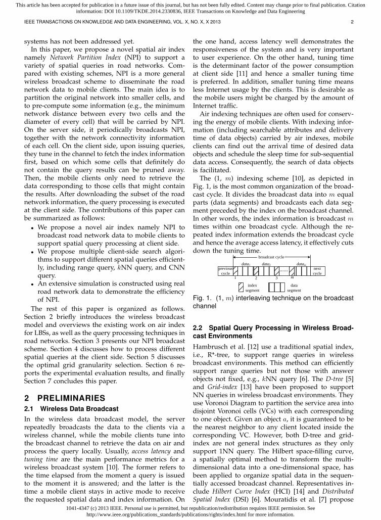
The (1, m) indexing scheme [10], as depicted inFig. 1, is the most common organization of the broad-cast cycle. It divides the broadcast data into m equalparts (data segments) and broadcasts each data seg-ment preceded by the index on the broadcast channel.In other words, the index information is broadcast mtimes within one broadcast cycle. Although the re-peated index information extends the broadcast cycleand hence the average access latency, it effectively cutsdown the tuning time.
index
segment
data
segment
……previous
cycle
next
cycle1 2 3 m
broadcast cycle
data1 data2 datam
Fig. 1. (1, m) interleaving technique on the broadcastchannel
2.2 Spatial Query Processing in Wireless Broad-cast Environments
Hambrusch et al. [12] use a traditional spatial index,i.e., R*-tree, to support range queries in wirelessbroadcast environments. This method can efficientlysupport range queries but not those with answerobjects not fixed, e.g., kNN query [6]. The D-tree [5]and Grid-index [13] have been proposed to supportNN queries in wireless broadcast environments. Theyuse Voronoi Diagram to partition the service area intodisjoint Voronoi cells (VCs) with each correspondingto one object. Given an object a, it is guaranteed to bethe nearest neighbor to any client located inside thecorresponding VC. However, both D-tree and grid-index are not general index structures as they onlysupport 1NN query. The Hilbert space-filling curve,a spatially optimal method to transform the multi-dimensional data into a one-dimensional space, hasbeen applied to organize spatial data in the sequen-tially accessed broadcast channel. Representatives in-clude Hilbert Curve Index (HCI) [14] and DistributedSpatial Index (DSI) [6]. Mouratidis et al. [7] propose
1041-4347 (c) 2013 IEEE. Personal use is permitted, but republication/redistribution requires IEEE permission. Seehttp://www.ieee.org/publications_standards/publications/rights/index.html for more information.
This article has been accepted for publication in a future issue of this journal, but has not been fully edited. Content may change prior to final publication. Citationinformation: DOI 10.1109/TKDE.2014.2330836, IEEE Transactions on Knowledge and Data Engineering
IEEE TRANSACTIONS ON KNOWLEDGE AND DATA ENGINEERING, VOL. X, NO. X, X 2013 3
the Broadcast Grid Index (BGI), which outperformsthe previous techniques in both static and dynamicenvironments. BGI uses grid cell as the index becausegrid cell is not only of small size but also very efficientfor objects updates.
However, all above-mentioned approaches onlyconsider the spatial queries in a Euclidean space. Inmany real life applications, the objects’ movementsare constrained in a road network. The index tech-niques such as R*-tree based method or grid cellcan’t be directly applied in road networks becausethe network distance (i.e., the shortest path distance)can’t be computed using only the boundary of theminimum boundary rectangle (MBR) or grid cell. Thesame problem occurs in the Voronoi-based techniqueand the Hilbert-curve based methods.
2.3 Spatial Query Processing in Road Networks
In general, a road network is modeled as an undirect-ed graph G(V,E), with V being the set of verticesand E being the set of edges. As road networksusually are sparse graphs, it is common to store Gusing adjacency lists. An edge (vi, vj) ∈ E representsthat vertices vi and vj are connected in the network.The weights of edges are captured by W . A non-negative weight w(vi, vj) ∈ W of edge (vi, vj) ∈ Ecan represent physical distance, travel time or othercosts according to different application context. Giventwo vertices vi and vj of a graph G(V,E), a pathand the shortest path connecting them are definedin Definition 1. In this paper, the distance (or thenetwork distance) between two vertices in a roadnetwork refers to their shortest distance.Definition 1: (Path and Shortest Path). Given a roadnetwork G(V,E) and vi, vj ∈ V , a path P (vi, vj)connecting vi and vj sequentially passes vertices vp1,vp2, · · ·, vpm, denoted as P (vi, vj) = {vi, vp1, vp2, · · ·,vpm, vj}. The length of P (vi, vj), denoted as |P (vi, vj)|,is∑mn=0 w(vpn, vp(n+1)) with vp0 = vi and vp(m+1) =
vj . The shortest path SP (vi, vj) is the one with theshortest length among all the paths from vi and vj ,and its length, denoted as ||vi, vj ||(= |SP (vi, vj)|), isthe network distance between vi and vj . �
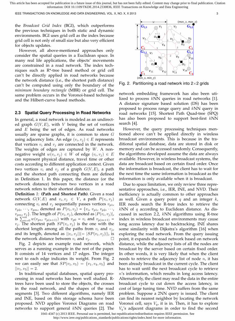
Fig. 2 depicts an example road network, whichserves as a running example in the rest of the paper.It consists of 14 vertices and 17 edges. The integernext to each edge indicates its weight. From Fig. 2we can easily see that SP (v1, v5) = {v1, v4, v5} and||v1, v5|| = 2.
In traditional spatial databases, spatial query pro-cessing in road networks has been well studied. R-trees have been used to store the objects, the crossesin the road network, and the shapes of the roadsegments [3]. Two different algorithms, namely IERand INE, based on this storage schema have beenproposed. NVD applies Voronoi Diagrams on roadnetworks to support general kNN queries [2]. The
(min_x, min_y)
v1 v2
1 1 1 1 1
11 1
v3
v4
v5 v6
v7
v8v9 v10
v11 v12 v13v14
3
2
3
21
11
11
(max_x, max_y)w
w
G1,1 G1,2
G2,1 G2,2
o4
0.8
0.2
o30.5
0.5
o1
0.6
0.4
o20.6 0.4
C2
C1
C3
C4
Fig. 2. Partitioning a road network into 2×2 grids
network embedding framework has also been uti-lized to process kNN queries in road networks [1].A distance signature based solution (DS) has beenproposed to process range query and kNN query inroad networks [15]. Shortest Path Quad-tree (SPQ)has also been proposed to support best-first kNNsearch [4].
However, the query processing techniques men-tioned above can’t be applied directly in wirelessbroadcast environments. This is because in the tra-ditional spatial database, data are stored in disk ormemory and can be accessed randomly. Consequently,the algorithms developed assume the data are alwaysavailable. However, in wireless broadcast systems, thedata are broadcast based on certain fixed order. Oncethe information is broadcast, the client has to wait forthe next time the same information is broadcast as theinformation is only available when it is broadcast.
Due to space limitation, we only review three repre-sentative approaches, i.e., IER, INE, and NVD. Theirinefficiency is actually common to other approachesas well. Given a query point q and an integer k,IER needs search the R-tree index to retrieve thekNN of q according to Euclidean distance. As dis-cussed in section 2.2, kNN algorithms using R-treeindex in wireless broadcast environments may causelong access latency due to backtracking. INE sharessome similarity with Dijkstra’s algorithm [16] whenexploring the road network. From the query issuingpoint, it expands the road network based on networkdistance, while the adjacency lists of all the nodes arebroadcast by the server based on certain fixed order.In other words, it is very likely that when the clientneeds to retrieve the adjacency list of node n, it hasbeen already broadcast in the current cycle. The clienthas to wait until the next broadcast cycle to retrieven’s information, which results in long access latency.Alternatively, the client may read the data in the entirebroadcast cycle to cut down the access latency, incost of large tuning time. NVD suffers from the sameproblem. Suppose a 2NN query is issued. The clientcan find its nearest neighbor by locating the networkVoronoi cell, says Vq , it is in. Then, it has to exploreVq’s adjacent diagrams in order to find the second
1041-4347 (c) 2013 IEEE. Personal use is permitted, but republication/redistribution requires IEEE permission. Seehttp://www.ieee.org/publications_standards/publications/rights/index.html for more information.
This article has been accepted for publication in a future issue of this journal, but has not been fully edited. Content may change prior to final publication. Citationinformation: DOI 10.1109/TKDE.2014.2330836, IEEE Transactions on Knowledge and Data Engineering
IEEE TRANSACTIONS ON KNOWLEDGE AND DATA ENGINEERING, VOL. X, NO. X, X 2013 4
nearest neighbor. However, some of the Vq’s adjacentdiagrams might be broadcast earlier than Vq in thecurrent broadcast cycle. The client has to either waituntil the next cycle or blindly retrieve all the datawithin one cycle.
The wireless broadcast model is first adopted byKellaris et al. [8] to provide LBSs in road networks.Two different methods, namely EB and NR, are pro-posed to support shortest path computation on air.An energy-efficient air index, namely BagIndex, hasalso been proposed to support shortest path queries.Both [8] and [9] only support shortest path queries butnot common spatial queries such as range query andkNN query. A more general index that can supportmultiple spatial queries is desired.
3 NPI: AIR INDEX FOR SPATIAL QUERYPROCESSING IN ROAD NETWORKS
The result of a spatial query often lies somewherenear the client’s location. For example, the 10 nearestrestaurants to a query point q are centered at q andthey are not far away from q. This is because: i) pointsof interest such as restaurants are usually very densein a real road network, and ii) the value of k postedby the mobile user won’t be too large because it ismeaningless and not practical for a mobile deviceto deal with hundreds or thousands of objects. Inother words, the client needs not to read the networkinformation too far away.
Motivated by this observation, we partition theoriginal road network into small regions and pre-compute certain information for each region, whichforms the index (i.e., NPI). The index information,as well as the adjacency lists of each region, is in-terleaved in the broadcast channel. In this section,we first introduce the network partition and someimportant concepts. Then, we present the informationcarried by NPI. Next, we discuss the content of thedata segment, i.e., the road network structure repre-sented by the adjacency lists as well as the objectslocation and description. Finally, we explain how tointerleave the index and data segment in a wirelesschannel.
3.1 Grid Partition of the Road NetworksThere are several strategies to partition the roadnetwork [17]. In this paper, we adopt the grid par-titioning algorithm for the size of a grid index isvery small. Other partition methods such as quadtreepartition and kd-tree partition can also be applied toour NPI. The road network is partitioned into n × n(= N ) equal-size grids. Here, n refers to the numberof grids in each dimension. All the grid cells Gi,j(1 ≤ i,j ≤ n) are in square shape with w being the sidelength. The header of NPI contains the grid partitioninformation, i.e., the minimum/maximum x/y coor-dinate of the service area (denoted as min x/min y,
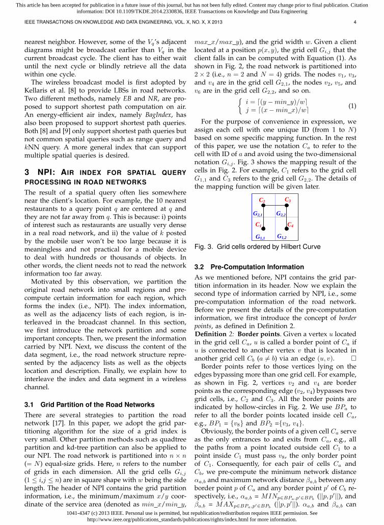
max x/max y), and the grid width w. Given a clientlocated at a position p(x, y), the grid cell Gi,j that theclient falls in can be computed with Equation (1). Asshown in Fig. 2, the road network is partitioned into2 × 2 (i.e., n = 2 and N = 4) grids. The nodes v1, v3,and v4 are in the grid cell G2,1, the nodes v2, v5, andv6 are in the grid cell G2,2, and so on.{
i = d(y −min y)/wej = d(x−min x)/we (1)
For the purpose of convenience in expression, weassign each cell with one unique ID (from 1 to N )based on some specific mapping function. In the restof this paper, we use the notation Ca to refer to thecell with ID of a and avoid using the two-dimensionalnotation Gi,j . Fig. 3 shows the mapping result of thecells in Fig. 2. For example, C1 refers to the grid cellG1,1 and C3 refers to the grid cell G2,2. The details ofthe mapping function will be given later.
G1,1 G1,2
G2,1 G2,2
C1
C2 C3
C4
Fig. 3. Grid cells ordered by Hilbert Curve
3.2 Pre-Computation InformationAs we mentioned before, NPI contains the grid par-tition information in its header. Now we explain thesecond type of information carried by NPI, i.e., somepre-computation information of the road network.Before we present the details of the pre-computationinformation, we first introduce the concept of borderpoints, as defined in Definition 2.Definition 2: Border points. Given a vertex u locatedin the grid cell Ca, u is called a border point of Ca ifu is connected to another vertex v that is located inanother grid cell Cb (a 6= b) via an edge (u, v). �
Border points refer to those vertices lying on theedges bypassing more than one grid cell. For example,as shown in Fig. 2, vertices v2 and v4 are borderpoints as the corresponding edge (v2, v4) bypasses twogrid cells, i.e., C2 and C3. All the border points areindicated by hollow-circles in Fig. 2. We use BPa torefer to all the border points located inside cell Ca,e.g., BP1 = {v8} and BP2 ={v3, v4}.
Obviously, the border points of a given cell Ca serveas the only entrances to and exits from Ca, e.g., allthe paths from a point located outside cell C1 to apoint inside C1 must pass v8, the only border pointof C1. Consequently, for each pair of cells Ca andCb, we pre-compute the minimum network distanceαa,b and maximum network distance βa,b between anyborder point p of Ca and any border point p′ of Cb re-spectively, i.e., αa,b = MINp∈BPa,p′∈BPb
(||p, p′||), andβa,b = MAXp∈BPa,p′∈BPb
(||p, p′||). αa,b and βa,b can
1041-4347 (c) 2013 IEEE. Personal use is permitted, but republication/redistribution requires IEEE permission. Seehttp://www.ieee.org/publications_standards/publications/rights/index.html for more information.
This article has been accepted for publication in a future issue of this journal, but has not been fully edited. Content may change prior to final publication. Citationinformation: DOI 10.1109/TKDE.2014.2330836, IEEE Transactions on Knowledge and Data Engineering
IEEE TRANSACTIONS ON KNOWLEDGE AND DATA ENGINEERING, VOL. X, NO. X, X 2013 5
facilitate the approximation of the network distancefrom a point in cell Ca to a point located in anothergrid cell Cb. This will be detailed in the next section.
Take the cells C2 and C4 in our example roadnetwork as an example. Since BP2 = {v3, v4} and BP4
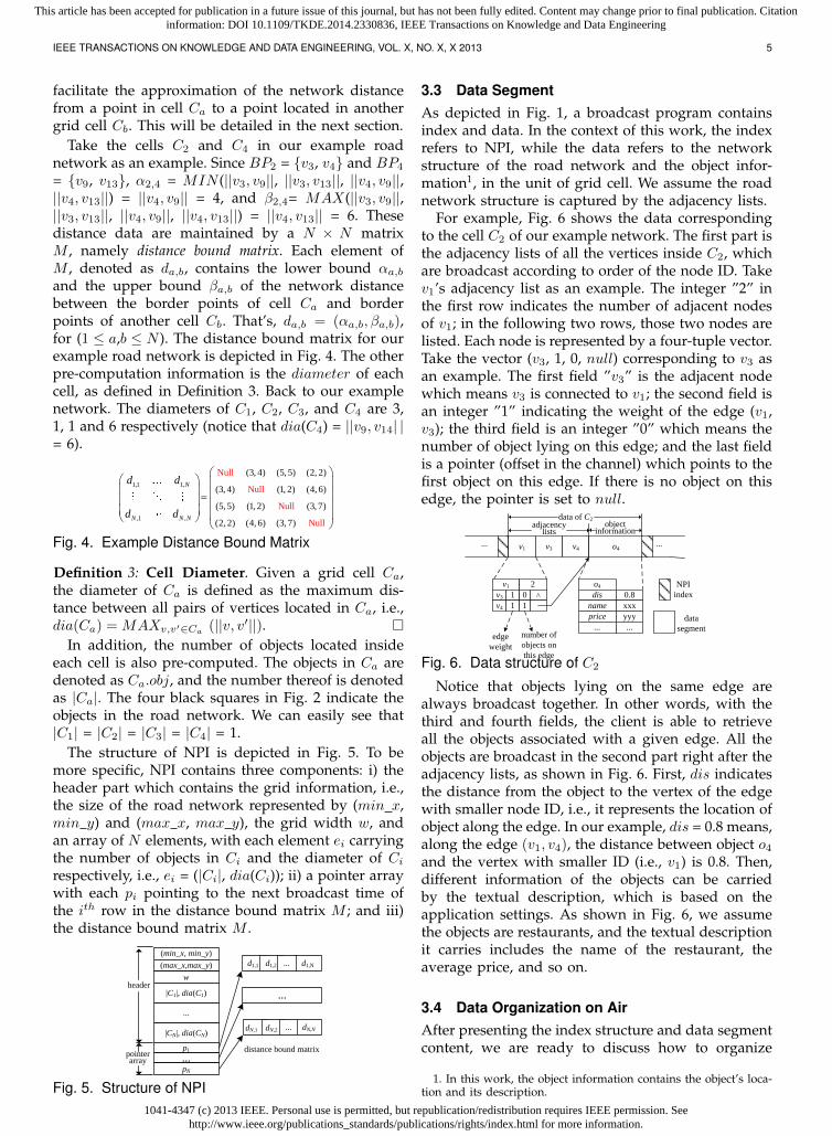
= {v9, v13}, α2,4 = MIN (||v3, v9||, ||v3, v13||, ||v4, v9||,||v4, v13||) = ||v4, v9|| = 4, and β2,4= MAX(||v3, v9||,||v3, v13||, ||v4, v9||, ||v4, v13||) = ||v4, v13|| = 6. Thesedistance data are maintained by a N × N matrixM , namely distance bound matrix. Each element ofM , denoted as da,b, contains the lower bound αa,band the upper bound βa,b of the network distancebetween the border points of cell Ca and borderpoints of another cell Cb. That’s, da,b = (αa,b, βa,b),for (1 ≤ a,b ≤ N ). The distance bound matrix for ourexample road network is depicted in Fig. 4. The otherpre-computation information is the diameter of eachcell, as defined in Definition 3. Back to our examplenetwork. The diameters of C1, C2, C3, and C4 are 3,1, 1 and 6 respectively (notice that dia(C4) = ||v9, v14| |= 6).
1,1 1,
,1 ,
(3, 4) (5, 5) (2, 2)
(3, 4) (1, 2) (4, 6)
(5, 5)
Null
Null
Nu(1, 2) (3, 7)
(2, 2) (4, 6) (3
ll
Nu7) ll,
N
N N N
d d
d d
Fig. 4. Example Distance Bound Matrix
Definition 3: Cell Diameter. Given a grid cell Ca,the diameter of Ca is defined as the maximum dis-tance between all pairs of vertices located in Ca, i.e.,dia(Ca) =MAXv,v′∈Ca
(||v, v′||). �In addition, the number of objects located inside
each cell is also pre-computed. The objects in Ca aredenoted as Ca.obj, and the number thereof is denotedas |Ca|. The four black squares in Fig. 2 indicate theobjects in the road network. We can easily see that|C1| = |C2| = |C3| = |C4| = 1.
The structure of NPI is depicted in Fig. 5. To bemore specific, NPI contains three components: i) theheader part which contains the grid information, i.e.,the size of the road network represented by (min x,min y) and (max x, max y), the grid width w, andan array of N elements, with each element ei carryingthe number of objects in Ci and the diameter of Cirespectively, i.e., ei = (|Ci|, dia(Ci)); ii) a pointer arraywith each pi pointing to the next broadcast time ofthe ith row in the distance bound matrix M ; and iii)the distance bound matrix M .
d1,N
(min_x, min_y)
(max_x,max_y)
p1
...pN
d1,1 d1,2 ...
...header
pointer array
|C1|, dia(C1)
...
|CN|, dia(CN)
w
distance bound matrix
dN,N...dN,1 dN,2
Fig. 5. Structure of NPI
3.3 Data SegmentAs depicted in Fig. 1, a broadcast program containsindex and data. In the context of this work, the indexrefers to NPI, while the data refers to the networkstructure of the road network and the object infor-mation1, in the unit of grid cell. We assume the roadnetwork structure is captured by the adjacency lists.
For example, Fig. 6 shows the data correspondingto the cell C2 of our example network. The first part isthe adjacency lists of all the vertices inside C2, whichare broadcast according to order of the node ID. Takev1’s adjacency list as an example. The integer ”2” inthe first row indicates the number of adjacent nodesof v1; in the following two rows, those two nodes arelisted. Each node is represented by a four-tuple vector.Take the vector (v3, 1, 0, null) corresponding to v3 asan example. The first field ”v3” is the adjacent nodewhich means v3 is connected to v1; the second field isan integer ”1” indicating the weight of the edge (v1,v3); the third field is an integer ”0” which means thenumber of object lying on this edge; and the last fieldis a pointer (offset in the channel) which points to thefirst object on this edge. If there is no object on thisedge, the pointer is set to null.
v1 v3 v4 o4
v1
v3
2
1 0
v4 1 1
adjacency lists
object information
data of C2
o4
dis 0.8
name
price
...
xxx
yyy
...edge
weight
number of
objects on
this edge
NPI
index
data
segment
... ...
^
Fig. 6. Data structure of C2
Notice that objects lying on the same edge arealways broadcast together. In other words, with thethird and fourth fields, the client is able to retrieveall the objects associated with a given edge. All theobjects are broadcast in the second part right after theadjacency lists, as shown in Fig. 6. First, dis indicatesthe distance from the object to the vertex of the edgewith smaller node ID, i.e., it represents the location ofobject along the edge. In our example, dis = 0.8 means,along the edge (v1, v4), the distance between object o4and the vertex with smaller ID (i.e., v1) is 0.8. Then,different information of the objects can be carriedby the textual description, which is based on theapplication settings. As shown in Fig. 6, we assumethe objects are restaurants, and the textual descriptionit carries includes the name of the restaurant, theaverage price, and so on.
3.4 Data Organization on AirAfter presenting the index structure and data segmentcontent, we are ready to discuss how to organize
1. In this work, the object information contains the object’s loca-tion and its description.
1041-4347 (c) 2013 IEEE. Personal use is permitted, but republication/redistribution requires IEEE permission. Seehttp://www.ieee.org/publications_standards/publications/rights/index.html for more information.
This article has been accepted for publication in a future issue of this journal, but has not been fully edited. Content may change prior to final publication. Citationinformation: DOI 10.1109/TKDE.2014.2330836, IEEE Transactions on Knowledge and Data Engineering
IEEE TRANSACTIONS ON KNOWLEDGE AND DATA ENGINEERING, VOL. X, NO. X, X 2013 6
them in a wireless channel. First, as the service areais partitioned into N grid cells, we need to decide thebroadcast order of grid cells. The order might not beimportant for some queries, but it has a direct impacton the performance of spatial query processing. Inthis paper, we use the Hilbert space filling curve asthe mapping function to sort grid cells into a one-dimensional space, which is widely used for spatialquery processing in wireless broadcast environmen-t [6], [7], [14]. Fig. 3 depicts the Hilbert curve fora (2 × 2) grid of our example road network. TheHilbert values for cell G1,1 and G2,2 are 1 and 3,respectively. According to [14], given a cell Gi,j , theclient can compute the Hilbert value of Gi,j in aconstant time. Moreover, as Hilbert curve can preservethe spatial locality, the cells with close Hilbert valuesare normally close to each other as well. In otherwords, the grid cells that contain the objects requestedby a user will appear closely in the wireless channel,which will facilitate the client’s data retrieval process.
We assume NPI is much smaller, compared with thedata segments, and hence we adopt (1, m) scheme asthe data organization strategy for better tuning timeperformance. Each index segment contains the entireNPI. The grid cells are ordered based on their Hilbertvalues, and their data are partitioned into m partswith each part carried by one data segment. In thebroadcast channel, we interleave index segments withdata segments, as shown in Fig. 1.
4 CLIENT-SITE QUERY PROCESSING
As explained before, the NPI enables the client toeasily get the following information:i) the distributionof the objects; ii) the approximate network distancefrom the query point to other grid cells and henceto the objects; and iii) the arrival time of the datain each grid cell. Based on the above information,clients can answer various kinds of spatial queries inroad networks. In this section, we discuss the searchalgorithms based on NPI for range queries, snapshotkNN queries, and continuous kNN queries.
The basic idea of the search algorithms is to firstlocate the grid cell containing the client and then toread the lower and upper bound of its distance toother grid cells. According to the distance bounds andthe distribution of the objects, the client can get thelocations of the candidate objects. Then, following theNPI, the clients can retrieve the cells containing thecandidate objects but ignore the rest. When the candi-date objects are locally available, the clients can locatethe result objects based on real network distance vialocal processing. Because the mobile clients usuallyask for nearby information (e.g., the range of rangequeries is normally small), the number of candidatecells is much smaller compared with the total numberof cells. In other words, the retrieved grid cells willform a sub-graph that is significantly smaller than the
original road network and it is practical for mobileclients to adopt some basic road network exploringtechniques for the local processing. In our simulation,we adopt Dijkstra’s algorithm because it is simpleand efficient in the small sub-graph downloaded byclients.
Before we present different search algorithms, wehighlight an important assumption we make. Likemany other existing works [4], [8], [9], we assumethe clients are located at network nodes to simplifyour discussion. However, our algorithms can be easilyextended to support cases where clients’ locations arelocated along the network edges.
4.1 Range queries
Given a query point q, a distance d and a dataset S in aroad network, a range query retrieves all the objectsin S that are within the network distance d from q,denoted as Range(q, d, S) = {o | o ∈ S ∧ ||o, q|| ≤d}. As the network distance between objects a and bwill not be shorter than the lower bound αi,j betweencells Ci and Cj with a ∈ Ci.obj and b ∈ Cj .obj (i.e.,||a, b| ≥ αi,j), only those cells Cn with their lowerbound distances αn,q to cell Cq bounded by d maycontain the result objects, i.e., Range(q, d, S) ⊆ {o | o∈⋃αn,q≤d Cn.obj}. The correctness of above statement
is guaranteed by Lemma 1.Lemma 1: Given a point q located at grid cell Cq anda grid cell Cn, if αn,q > d, the network distance fromany object inside Cn to q is larger than d, i.e., q ∈ Cq∧ αn,q > d ⇒ ∀ o ∈ Cn.obj, ||o, q|| ≥ αn,q > d. �Proof. The proof is straightforward and hence it isignored for space saving. �
Algorithm 1 : NPI-based Range Query Processing on AirInput: a source point q, a value d and a dataset SOutput: Range(q, d, S)Procedure:1: TuneIntoChannel();2: NPIHeader ← retrieveIndexHeader();3: locate the grid cell Cq containing q;4: read the qth row Rq corresponding to Cq in the matrix;5: for each cell Ci do6: if αq,i ≤ d then add Ci to the candidate cells;7: sort the candidate cells by their arrival time;8: for each candidate cell do9: sleepUntilCellBroadcast();
10: TuneIntoChannel();11: adjacencyLists← retrieveCell();12: subGraph.add(adjacencyLists);13: return DijkstraExpansion(subGraph, q, d);
Based on above finding, the algorithm for sup-porting range query is straightforward. We adoptthe filtering-and-refinement strategy, and Algorithm 1lists its pseudo-code. In the filtering phase, the clientlistens to NPI. It locates the cell Cq it lies in based onits location and the grid partition information, andthen fetches the qth row of the distance bound matrix(lines 1-4). Based on αi,q , it can decide all the cells
1041-4347 (c) 2013 IEEE. Personal use is permitted, but republication/redistribution requires IEEE permission. Seehttp://www.ieee.org/publications_standards/publications/rights/index.html for more information.
This article has been accepted for publication in a future issue of this journal, but has not been fully edited. Content may change prior to final publication. Citationinformation: DOI 10.1109/TKDE.2014.2330836, IEEE Transactions on Knowledge and Data Engineering
IEEE TRANSACTIONS ON KNOWLEDGE AND DATA ENGINEERING, VOL. X, NO. X, X 2013 7
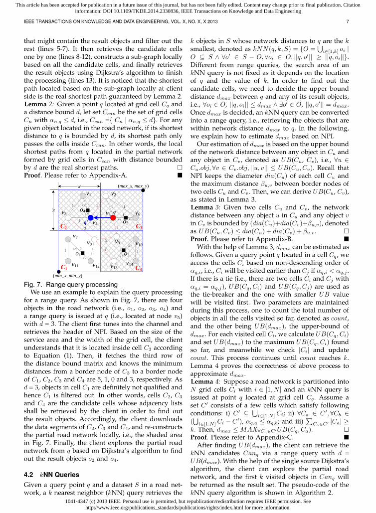
that might contain the result objects and filter out therest (lines 5-7). It then retrieves the candidate cellsone by one (lines 8-12), constructs a sub-graph locallybased on all the candidate cells, and finally retrievesthe result objects using Dijkstra’s algorithm to finishthe processing (lines 13). It is noticed that the shortestpath located based on the sub-graph locally at clientside is the real shortest path guaranteed by Lemma 2.Lemma 2: Given a point q located at grid cell Cq anda distance bound d, let set Ccan be the set of grid cellsCn with αn,q ≤ d, i.e., Ccan ={ Cn | αn,q ≤ d}. For anygiven object located in the road network, if its shortestdistance to q is bounded by d, its shortest path onlypasses the cells inside Ccan. In other words, the localshortest paths from q located in the partial networkformed by grid cells in Ccan with distance boundedby d are the real shortest paths. �Proof. Please refer to Appendix-A. �
(min_x, min_y)
v1 v2
1 1 1 1 1
11 1
v3
v4
v5 v6
v7
v8v9 v10
v11 v12 v13v14
3
2
3
21
11
11
(max_x, max_y)w
w o4
0.8
0.2
o30.5
0.5
o1
0.6
0.4
o20.6 0.4
C2
C1
C3
C4
q
q’
Fig. 7. Range query processingWe use an example to explain the query processing
for a range query. As shown in Fig. 7, there are fourobjects in the road network (i.e., o1, o2, o3, o4) anda range query is issued at q (i.e., located at node v5)with d = 3. The client first tunes into the channel andretrieves the header of NPI. Based on the size of theservice area and the width of the grid cell, the clientunderstands that it is located inside cell C3 accordingto Equation (1). Then, it fetches the third row ofthe distance bound matrix and knows the minimumdistances from a border node of C3 to a border nodeof C1, C2, C3 and C4 are 5, 1, 0 and 3, respectively. Asd = 3, objects in cell C1 are definitely not qualified andhence C1 is filtered out. In other words, cells C2, C3
and C4 are the candidate cells whose adjacency listsshall be retrieved by the client in order to find outthe result objects. Accordingly, the client downloadsthe data segments of C2, C3 and C4, and re-constructsthe partial road network locally, i.e., the shaded areain Fig. 7. Finally, the client explores the partial roadnetwork from q based on Dijkstra’s algorithm to findout the result objects o2 and o4.
4.2 kNN QueriesGiven a query point q and a dataset S in a road net-work, a k nearest neighbor (kNN) query retrieves the
k objects in S whose network distances to q are the ksmallest, denoted as kNN(q, k, S) = {O =
⋃i∈[1,k] oi |
O ⊆ S ∧ ∀o′ ∈ S − O,∀oi ∈ O, ||q, o′|| ≥ ||q, oi||}.Different from range queries, the search area of ankNN query is not fixed as it depends on the locationof q and the value of k. In order to find out thecandidate cells, we need to decide the upper bounddistance dmax between q and any of its result objects,i.e., ∀oi ∈ O, ||q, oi|| ≤ dmax ∧ ∃o′ ∈ O, ||q, o′|| = dmax.Once dmax is decided, an kNN query can be convertedinto a range query, i.e., retrieving the objects that arewithin network distance dmax to q. In the following,we explain how to estimate dmax based on NPI.
Our estimation of dmax is based on the upper boundof the network distance between any object in Cu andany object in Cv , denoted as UB(Cu, Cv), i.e., ∀u ∈Cu.obj,∀v ∈ Cv.obj, ||u, v|| ≤ UB(Cu, Cv). Recall thatNPI keeps the diameter dia(Cu) of each cell Cu andthe maximum distance βu,v between border nodes oftwo cells Cu and Cv . Then, we can derive UB(Cu, Cv),as stated in Lemma 3.Lemma 3: Given two cells Cu and Cv , the networkdistance between any object u in Cu and any object vin Cv is bounded by (dia(Cu)+dia(Cv)+βu,v), denotedas UB(Cu, Cv) ≤ dia(Cu) + dia(Cv) + βu,v . �Proof. Please refer to Appendix-B. �
With the help of Lemma 3, dmax can be estimated asfollows. Given a query point q located in a cell Cq , weaccess the cells Ci based on non-descending order ofαq,i, i.e., Ci will be visited earlier than Cj if αq,i < αq,j .If there is a tie (i.e., there are two cells Ci and Cj withαq,i = αq,j), UB(Cq, Ci) and UB(Cq, Cj) are used asthe tie-breaker and the one with smaller UB valuewill be visited first. Two parameters are maintainedduring this process, one to count the total number ofobjects in all the cells visited so far, denoted as count,and the other being UB(dmax), the upper-bound ofdmax. For each visited cell Ci, we calculate UB(Cq, Ci)and set UB(dmax) to the maximum UB(Cq, Ci) foundso far, and meanwhile we check |Ci| and updatecount. This process continues until count reaches k.Lemma 4 proves the correctness of above process toapproximate dmax.Lemma 4: Suppose a road network is partitioned intoN grid cells Ci with i ∈ [1, N ] and an kNN query isissued at point q located at grid cell Cq . Assume aset C ′ consists of a few cells which satisfy followingconditions: i) C ′ ⊆
⋃i∈[1,N ] Ci; ii) ∀Ca ∈ C ′,∀Cb ∈
(⋃i∈[1,N ] Ci − C ′), αq,a ≤ αq,b; and iii)
∑Ca∈C′ |Ca| ≥
k. Then, dmax ≤MAX∀Ca∈C′UB(Cq, Ca). �Proof. Please refer to Appendix-C. �
After finding UB(dmax), the client can retrieve thekNN candidates Canq via a range query with d =UB(dmax). With the help of the single source Dijkstra’salgorithm, the client can explore the partial roadnetwork, and the first k visited objects in Canq willbe returned as the result set. The pseudo-code of thekNN query algorithm is shown in Algorithm 2.
1041-4347 (c) 2013 IEEE. Personal use is permitted, but republication/redistribution requires IEEE permission. Seehttp://www.ieee.org/publications_standards/publications/rights/index.html for more information.
This article has been accepted for publication in a future issue of this journal, but has not been fully edited. Content may change prior to final publication. Citationinformation: DOI 10.1109/TKDE.2014.2330836, IEEE Transactions on Knowledge and Data Engineering
IEEE TRANSACTIONS ON KNOWLEDGE AND DATA ENGINEERING, VOL. X, NO. X, X 2013 8
Algorithm 2 : NPI-based kNN Query Processing on AirInput: a source point q, an integer k and a dataset SOutput: k objects in S closest to qProcedure:1: Q← ∅, count← 0, UB(dmax)← 0;2: TuneIntoChannel();3: NPIHeader ← retrieveIndexHeader();4: locate the grid cell Cq containing q;5: read the qth row Rq corresponding to Cq in the matrix;6: sort the cells Ci based on non-descending order of αq,i
and maintained in Q;7: while Q is not empty do8: Ci ← Q.pop();9: count← count+ |Ci|;
10: UB(dmax)←MAX(UB(dmax), UB(Cq, Ci));11: if count ≥ k then break;12: (subGraph, Canq) ← rangeQuery(q, UB(dmax), S);13: return DijkstraExpansion(subGraph, Canq , q, k);
Recall the example in Fig. 7. Suppose a 2NNquery is issued at q. The client first needs to findout UB(dmax). It first locates the cell C3 it liesin, and visits the cells Ci in the order of (C3, C2,C4, C1), following the non-descending order of α3,i.As |C3| = 1 and |C2| = 1 (i.e., |C3| + |C2| = k),UB(dmax) is set to MAX(UB(C3, C3), UB(C3, C2)) =MAX(dia(C3), dia(C3) + dia(C2) + β3,2) = dia(C3) +dia(C2) + β3,2 = 4. Next, the client needs to retrieveall the cells Ci with α3,i ≤ UB(dmax), i.e., cells C2, C3
and C4, to construct the partial road network locally.Finally, with Dijkstra’s algorithm, the first two visitedobjects o2 and o4 are returned as the result objects.
4.3 Continuous NN QueriesIn real applications, mobile users might issue querieswhen they are moving. For example, a taxi drivermay keep asking for the closest client while he/sheis driving. This is known as the continuous nearestneighbor (CNN) queries [18], [19]. Given a query pathP (v1, v2, . . . , vL) in a road network, the CNN queryfinds a set of kNN results corresponding to eachsegment (namely valid interval) in P . The kNN resultsof all query points lying on one valid interval areidentical, and the start/end points of all the validintervals are called split points. A naive solution tosupport CNN queries is to continuously issue kNNqueries along each moving point. However, it is notefficient as the answers to kNN queries issued atnearby locations might be same. Consequently, a moreefficient search algorithm is needed to support CNNqueries.
Recall that kNN search algorithm presented aboveutilizes the parameter UB(dmax) to find the answerobjects. Given two kNN queries issued at two dif-ferent locations within the same grid cell, they sharethe same UB(dmax). In other words, the NPI-basedkNN search algorithm only considers the grid cellwhere the query is issued, but not the exact locationof the query point. That is to say the kNN candidates
and the partial road network remain the same if theclient does not move out of the current grid cell.Consequently, if the client issues kNN queries whenmoving, she/he needs not tune into the channel todownload new candidates or new adjacency lists ifshe/he is still within the current grid cell. We also findthat even if the client leaves the current grid cell buthas not moved a long distance, the kNN candidatesand partial road network will still remain the same,as stated in Lemma 5 and Lemma 6.Lemma 5: Given a query point q, let UB(dmax) be theupper bound calculated using Lemma 3 and Lem-ma 4, Canq be the set of kNN candidates returnedby algorithm 2, and dk be the distance from q toits kth NN. For a new query point q′, if ||q, q′|| ≤(UB(dmax)−dk)/2, then Canq contains q′’s kNN, i.e.,||q, q′|| ≤ UB(dmax)−dk
2 ⇒ kNN(q′, k, S) ⊆ Canq . �Proof. Please refer to Appendix-D. �Lemma 6: Assume q and q′ satisfy all the conditionsspecified in Lemma 5, and let G′ be the partial roadnetwork downloaded for kNN search at the querypoint q. The shortest path from q′ to its kNN won’tpass a node outside G′. �Proof. The proof is straightforward based on the proofof Lemma 2 and Lemma 5, and hence it is ignored forspace saving. �
Continue the example 2NN query depicted in Fig. 7with UB(dmax) = 4, the partial road network G′
formed by cells C2, C3 and C4, Canq = {o2, o3, o4},and dk = ||q, o4‖| = 1.2. Suppose the client movesto a new location v4. Although v4 is located in adifferent grid cell, the moving distance ||v4, v5|| = 1 <(UB(dmax) − dk)/2. Consequently, the 2NN of q′ isstill within Canq and G′ remains valid. If the movingdistance of the client exceeds (UB(dmax) − dk)/2,the client needs to tune into the channel to get thenew kNN candidates and retrieve new partial roadnetwork. At the downloading step, if the new partialroad network overlaps with the former one, we canignore the retrieval of the overlapped portion as it islocally available.
Accordingly, we propose to decompose a givenCNN query path P (v1, v2, . . . , vL) into disjoint spacevalid segments, denoted as SV S1, SV S2, . . . , SV Sl, andall the query points lying on a space valid segmentshare the same kNN candidates and partial roadnetwork. In other words, the client only needs to issuean kNN query at the starting point of a space validsegment to retrieve the kNN candidates and partialroad network. For the rest points along the spacevalid segment, no downloading from the wirelesschannel is necessary. The pseudo-code of the querypath decomposition is depicted in Algorithm 3 inAppendix-E. We want to highlight that this step is thekey of our CNN algorithm, which helps to reduce thetuning time and shorten access latency significantly.
Suppose a given query path is decomposed intoseveral space valid segments, we now explain how to
1041-4347 (c) 2013 IEEE. Personal use is permitted, but republication/redistribution requires IEEE permission. Seehttp://www.ieee.org/publications_standards/publications/rights/index.html for more information.
This article has been accepted for publication in a future issue of this journal, but has not been fully edited. Content may change prior to final publication. Citationinformation: DOI 10.1109/TKDE.2014.2330836, IEEE Transactions on Knowledge and Data Engineering
IEEE TRANSACTIONS ON KNOWLEDGE AND DATA ENGINEERING, VOL. X, NO. X, X 2013 9
process CNN locally for a given space valid segment.We adopt the approach proposed in [18] to furtherdecompose a space valid segment into several validintervals via split points. Given the fact that the resultset remains the same for CNN queries issued at anypoint along a valid interval, we only invoke an kNNquery at the starting point of a valid interval.
4.4 Handling of Network Link ErrorsIt is well-known that wireless communication is inher-ently unreliable and error-prone. Consequently, it isdesirable that query processing techniques proposedfor wireless broadcast systems are error-resilient andclients are able to resume the query processing easi-ly [6]. However, error-resilience is not the main focusof NPI air index proposed in this work, although itis one of the main directions for our future work. Asexplained previously, a client needs to download boththe index information and the grid cell data in order tofinish a query. In case the index is lost, the client needsto wait until the next time the index is broadcast. Aswe adopt (1, m) scheme to interleave the index withthe data, the client needs to wait for 1
m cycle until thenext instance of index is broadcast. In case the data(i.e., grid cell data) is lost, the client has to wait forone cycle until the same data is re-broadcast in thenext cycle.
5 GRID GRANULARITY SELECTIONNotice that all the algorithms we develop are basedon the pre-computed distance bound information. Themore precise the distance bound is, the more powerfulthe pruning is, the less the information retrieval isand hence the more efficient the query processing is.Obviously, the grid size directly affects the precisionof the distance bounds. In an extreme case where eachgrid contains at most one point, the distance boundreflects the real network distance between any twopoints. In order to facilitate the selection of a propergrid size, we develop an analytical model to analyzethe impact of grid size on the system performance.
Intuitively, a fine granularity achieves tighter boundof the search space but leads to larger index size.Both the size of the index and the size of grid cellsaffect the tuning time and access latency, so there is atradeoff between different grid partitions. Recall thatwe always partition the entire road network into 2i×2iuniform grids, in purpose of utilizing the Hilbertcurve. Let PSi be a uniform partitioning strategythat partitions the service area into 2i × 2i uniformgrids. For simplicity, we assume that both the nodesand the objects of the road network are uniformlydistributed in each grid cell. Let DS be the data size(in Bytes) of the entire road network, including theadjacency lists and the object information. Then thedata size of each grid GSi of PSi is DS
2i×2i = DS4i .
For the index size, as depicted in Fig. 5, assume
that both the number of objects (i.e., |Ci|) and thedistance between two points (i.e., dia(Ci), αa,b, andβa,b) occupy 4 Bytes, then the size of the NPI indexISi is 12NGi+8NG2
i = 4i+1(3+2×4i). As we employthe (1, m) index scheme, the cycle length of PSi is
Cyclei = DS +m× ISi.
Let r be the average query scope of all range queries(notice that an kNN query is also answered via arange query), and Readi be the number of grids of PSithat downloaded by a range query with radius of r.As the approximation of Readi for r in road networksis affected by many factors, it makes the analysis verycomplicated. In this paper, we simplify the analysisby using the Euclidean space and assume that r ≤ wi
2 .Assume that the road network in embedded in a L×LEuclidean space, then for a partition strategy PSi, thewidth of a grid wi = L
2i . For a range query with radiusr, Equation (2) states the expected number of gridsretrieved and its proof is presented in Appendix-F.
Readi = 1 +4r
wi+πr2
wi2(2)
Let TTi and ATi be the tuning time and accesslatency of a range query with radius of r respectively,we have TTi = ISi + Readi × GSi, and ATi =Cyclei+Readi×GSi
2 . Assume we use the Equation (3)to evaluate the performance of a a wireless databroadcast system, where α ∈ (0, 1) is a parameter tobalance tuning time and access latency.
Systemi = α× TTi + (1− α)ATi, (3)
Let t = 2i, based on the above analysis we have
Systemi = 4(2α+m−mα)t4 + 6(2α+m−mα)t2
+ 2r·DS·(3−α)L·t + DS·(3−α)
2t2 + L2·DS·(1−α)+πr2·DS·(3−α)2L2
(4)From Equation (4), we estimate the formulation of
Systemi, a function of i. By computing the minimumobjective function value of Equation (4) and gainingthe value of i accordingly, we can select the opti-mal grid granularity. The derivative of Systemi isa polynomial with power higher than 5. Accordingto the Abel-Ruffini theorem [20], there is no generalalgebraic solution to polynomial equations of degree5 or higher, so there is no formula of the optimal i andwe present the optimal selecting result in Section 6.
6 EVALUATIONIn this section, we conduct extensive experimentsto evaluate the performance of NPI for supportingrange queries, kNN queries, and CNN queries inroad networks. Some state-of-the-art road-networkquery processing techniques are implemented as thecompetitors, including RNE and INE algorithms [3],NVD algorithm [2], and NGE algorithm [1]. All thealgorithms were implemented in C++, and the perfor-mance evaluation is simulated on a Genuine Intel(R)
1041-4347 (c) 2013 IEEE. Personal use is permitted, but republication/redistribution requires IEEE permission. Seehttp://www.ieee.org/publications_standards/publications/rights/index.html for more information.
This article has been accepted for publication in a future issue of this journal, but has not been fully edited. Content may change prior to final publication. Citationinformation: DOI 10.1109/TKDE.2014.2330836, IEEE Transactions on Knowledge and Data Engineering
IEEE TRANSACTIONS ON KNOWLEDGE AND DATA ENGINEERING, VOL. X, NO. X, X 2013 10
1.80GHz PC with 3.00G RAM, running Microsoft Win-dows 7 Ultimate. We first briefly describe the exper-imental settings, and then present the experimentalresults.
6.1 Experimental SetupTwo real road network datasets are used in our simu-lation. They are the City of Oldenburg (OL) RoadNetwork and the California (CAL) Road Networkfrom [21]. The OL road network contains 6105 nodesand 7035 edges, while CAL consists of 21048 nodesand 21693 edges. For each road network, a set of ob-jects are randomly generated and uniformly distribut-ed over the network. Even though our frameworkcan handle objects of different sizes, for the sake ofsimplicity, we fix the size of an object at 128 bytes.
The evaluation is run on a simulator which consistsof a server, a client and a broadcast channel. The ser-ver pre-computes the distance bound matrix and thediameter of each cell. The pre-computation informa-tion along with the road network data is broadcast onthe channel repeatedly. We run only one client in oursimulation for simplicity, because the number of theclients will not affect the performance of a broadcastsystem. For each set of experiments, 400 randomlyissued queries are evaluated and the average perfor-mance is reported. As mentioned before, we assumethe query issuing points are always at the networknodes although our algorithms can be easily extendedto support cases where queries are issued along theedges. We adopt both the access latency (AT) andtuning time (TT) as the main performance metrics.For simplicity, we assume the bandwidth is fixed andmeasure AT and TT in terms of number of bytes ofthe data transferred in the wireless channel instead ofactual clock time in the client side.
In our experimental studies, we mainly considerthe impacts caused by four parameters. They arethe number of results k asked by kNN queries, thedistance d of range queries, the object density, andthe number of grid cells N . Table 1 lists their valueswith the underlined values standing for the defaultsettings. Notice that DN refers to the diameter of theroad network, |S| refers to the number of object setS, and |V | refers to the number of nodes in the roadnetwork. Without loss of generality, we vary the valueof one parameter in each set of experiments while theother three parameters are set at their defaults.
TABLE 1Parameter settings
Parameter Settingk 1, 5, 10, 15Query scope (d/DN ) 0.01, 0.05, 0.1, 0.2Object density (|S| / |V |) 0.01, 0.05, 0.1, 0.2Number of cells(N ) 16, 64, 256
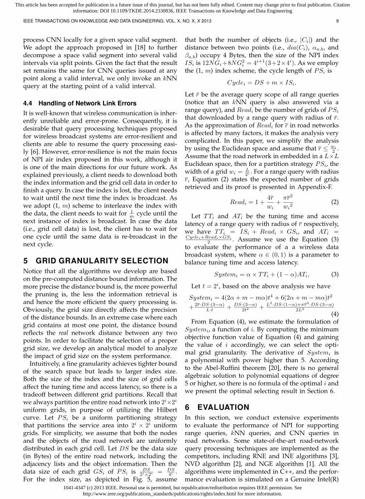
6.2 Cycle LengthFirst, we report the broadcast cycle length of differentindexes. We use OL dataset with the object density
set to 0.1. Here, a broadcast cycle consists of the indexand the data with data referring to the structure ofthe road network and the object information. BothRNE and INE are based on Dijkstra’s algorithm, sothey do not maintain any special index and employthe adjacency lists of all nodes to represent the roadnetwork. NGE carries the distance vector of eachnode in its index, and the number of reference nodesis set to 10 that is the default setting used by [1].NVD maintains the Voronoi cells of all the objectsin the road network as its index. NPI broadcastgrid partition information and some pre-computeddistance information in its index. As its size isdetermined by the number of grid cells, we testthe performance of NPI with 42, 43, 44 grid cells,denoted as NPI-16, NPI-64, and NPI-256 respectively.Notice that we set the number of grid cells as 4i isto simplify the Hilbert-Curve based ordering. ExceptRNE and INE, we adopt (1, m) scheme to generatethe broadcast program with the value of m set to itsoptimal value [10].
TABLE 2Broadcast cycle length
Method Indexsize(byte)
Datasize(byte)
Cyclelength(byte)
RNE/INE 0 367764 367764NGE-10 244200 367764 611964NVD 1152045 76800 1076800NPI-16 2196 367764 389724NPI-64 33300 367764 700764NPI-256 526356 367764 5631324
The experimental result is listed in Table 2. It isobserved that RNE and INE have the smallest cycle,because they do not maintain any index. Amongother schemes, NPI-16 has a pretty small index and itsbroadcast cycle length is very close to that of RNE andINE. Both NGE and NVD have relatively long broadcastcycle which is mainly caused by the large size ofthe index. The cycle length has a direct impact onthe access latency. Our following experimental studieswill further verify this.
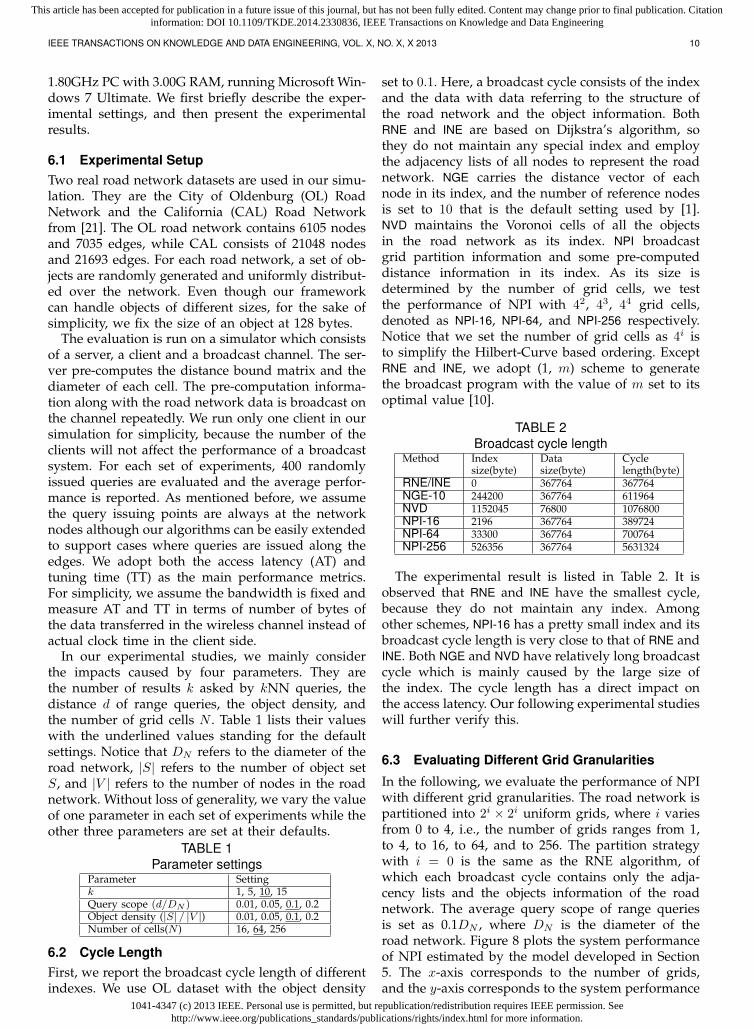
6.3 Evaluating Different Grid Granularities
In the following, we evaluate the performance of NPIwith different grid granularities. The road network ispartitioned into 2i × 2i uniform grids, where i variesfrom 0 to 4, i.e., the number of grids ranges from 1,to 4, to 16, to 64, and to 256. The partition strategywith i = 0 is the same as the RNE algorithm, ofwhich each broadcast cycle contains only the adja-cency lists and the objects information of the roadnetwork. The average query scope of range queriesis set as 0.1DN , where DN is the diameter of theroad network. Figure 8 plots the system performanceof NPI estimated by the model developed in Section5. The x-axis corresponds to the number of grids,and the y-axis corresponds to the system performance
1041-4347 (c) 2013 IEEE. Personal use is permitted, but republication/redistribution requires IEEE permission. Seehttp://www.ieee.org/publications_standards/publications/rights/index.html for more information.
This article has been accepted for publication in a future issue of this journal, but has not been fully edited. Content may change prior to final publication. Citationinformation: DOI 10.1109/TKDE.2014.2330836, IEEE Transactions on Knowledge and Data Engineering
IEEE TRANSACTIONS ON KNOWLEDGE AND DATA ENGINEERING, VOL. X, NO. X, X 2013 11
Systemi = α×TTi+(1−α)ATi. For different broadcastsystems may have different preferences to tuning timeand access latency, we vary the parameter α from13 , to 1
2 , and to 23 . From Figure 8 we can see that
partition strategies with 16 or 64 grids gain the bestperformance for different α. The correctness of themodel will be further demonstrated in the followingexperiments where we can get the real performanceof NPI with different grid partition granularities.
1000
2000
3000
1 4 16 64 256N
Syst
emi
(a) CAL
1 4 16 64 256N
5001000150020002500
Syst
emi
(b) OL
Fig. 8. Evaluation on grid granularity selection
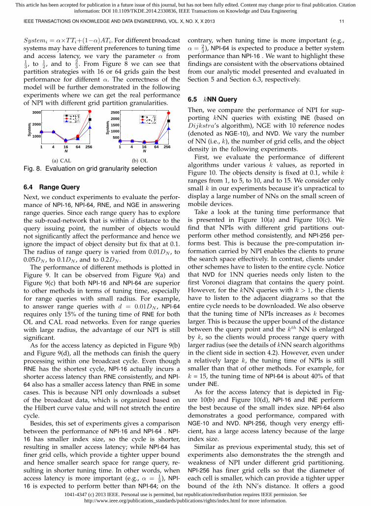
6.4 Range QueryNext, we conduct experiments to evaluate the perfor-mance of NPI-16, NPI-64, RNE, and NGE in answeringrange queries. Since each range query has to explorethe sub-road-network that is within d distance to thequery issuing point, the number of objects wouldnot significantly affect the performance and hence weignore the impact of object density but fix that at 0.1.The radius of range query is varied from 0.01DN , to0.05DN , to 0.1DN , and to 0.2DN .
The performance of different methods is plotted inFigure 9. It can be observed from Figure 9(a) andFigure 9(c) that both NPI-16 and NPI-64 are superiorto other methods in terms of tuning time, especiallyfor range queries with small radius. For example,to answer range queries with d = 0.01DN , NPI-64requires only 15% of the tuning time of RNE for bothOL and CAL road networks. Even for range querieswith large radius, the advantage of our NPI is stillsignificant.
As for the access latency as depicted in Figure 9(b)and Figure 9(d), all the methods can finish the queryprocessing within one broadcast cycle. Even thoughRNE has the shortest cycle, NPI-16 actually incurs ashorter access latency than RNE consistently, and NPI-64 also has a smaller access latency than RNE in somecases. This is because NPI only downloads a subsetof the broadcast data, which is organized based onthe Hilbert curve value and will not stretch the entirecycle.
Besides, this set of experiments gives a comparisonbetween the performance of NPI-16 and NPI-64 . NPI-16 has smaller index size, so the cycle is shorter,resulting in smaller access latency; while NPI-64 hasfiner grid cells, which provide a tighter upper boundand hence smaller search space for range query, re-sulting in shorter tuning time. In other words, whenaccess latency is more important (e.g., α = 1
3 ), NPI-16 is expected to perform better than NPI-64; on the
contrary, when tuning time is more important (e.g.,α = 2
3 ), NPI-64 is expected to produce a better systemperformance than NPI-16 . We want to highlight thesefindings are consistent with the observations obtainedfrom our analytic model presented and evaluated inSection 5 and Section 6.3, respectively.
6.5 kNN Query
Then, we compare the performance of NPI for sup-porting kNN queries with existing INE (based onDijkstra’s algorithm), NGE with 10 reference nodes(denoted as NGE-10), and NVD. We vary the numberof NN (i.e., k), the number of grid cells, and the objectdensity in the following experiments.
First, we evaluate the performance of differentalgorithms under various k values, as reported inFigure 10. The objects density is fixed at 0.1, while kranges from 1, to 5, to 10, and to 15. We consider onlysmall k in our experiments because it’s unpractical todisplay a large number of NNs on the small screen ofmobile devices.
Take a look at the tuning time performance thatis presented in Figure 10(a) and Figure 10(c). Wefind that NPIs with different grid partitions out-perform other method consistently, and NPI-256 per-forms best. This is because the pre-computation in-formation carried by NPI enables the clients to prunethe search space effectively. In contrast, clients underother schemes have to listen to the entire cycle. Noticethat NVD for 1NN queries needs only listen to thefirst Voronoi diagram that contains the query point.However, for the kNN queries with k > 1, the clientshave to listen to the adjacent diagrams so that theentire cycle needs to be downloaded. We also observethat the tuning time of NPIs increases as k becomeslarger. This is because the upper bound of the distancebetween the query point and the kth NN is enlargedby k, so the clients would process range query withlarger radius (see the details of kNN search algorithmsin the client side in section 4.2). However, even undera relatively large k, the tuning time of NPIs is stillsmaller than that of other methods. For example, fork = 15, the tuning time of NPI-64 is about 40% of thatunder INE.
As for the access latency that is depicted in Fig-ure 10(b) and Figure 10(d), NPI-16 and INE performthe best because of the small index size. NPI-64 alsodemonstrates a good performance, compared withNGE-10 and NVD. NPI-256, though very energy effi-cient, has a large access latency because of the largeindex size.
Similar as previous experimental study, this set ofexperiments also demonstrates the the strength andweakness of NPI under different grid partitioning.NPI-256 has finer grid cells so that the diameter ofeach cell is smaller, which can provide a tighter upperbound of the kth NN’s distance. It offers a good
1041-4347 (c) 2013 IEEE. Personal use is permitted, but republication/redistribution requires IEEE permission. Seehttp://www.ieee.org/publications_standards/publications/rights/index.html for more information.
This article has been accepted for publication in a future issue of this journal, but has not been fully edited. Content may change prior to final publication. Citationinformation: DOI 10.1109/TKDE.2014.2330836, IEEE Transactions on Knowledge and Data Engineering
IEEE TRANSACTIONS ON KNOWLEDGE AND DATA ENGINEERING, VOL. X, NO. X, X 2013 12
0.01 0.05 0.10 0.15 0.200
150
300
450
600Tu
ning
Tim
e(KB
)
radius
RNE NGE-10 NPI-16 NPI-64
(a) Tuning Time(OL)
0.01 0.05 0.10 0.15 0.20300
400
500
600
Acce
ss L
aten
cy(K
B)
radius
RNE NGE-10 NPI-16 NPI-64
(b) Access Latency(OL)
0.01 0.05 0.10 0.15 0.200
500
1000
1500
2000
Tuni
ng T
ime(
KB)
radius
RNE NGE-10 NPI-16 NPI-64
(c) Tuning Time(CAL)
0.01 0.05 0.10 0.15 0.20900
1200
1500
1800
2100
Acce
ss L
aten
cy(K
B)
radius
RNE NGE-10 NPI-16 NPI-64
(d) Access Latency(CAL)
Fig. 9. Performance of range query vs. radius
1
INE NGE-10 NPI-16 NPI-64 NPI-256 NVD
5 10 1550
350
650
950
1250
Tuni
ng T
ime(
KB)
k
(a) Tuning Time(OL)
1 5 10 15200
1200
2200
3200
4200
Acce
ss L
aten
cy(K
B)
k
INE NGE-10 NPI-16 NPI-64 NPI-256 NVD
(b) Access Latency(OL)
1
RNE NGE-10 NPI-16 NPI-64 NPI-256 NVD
5 10 150
1000
2000
3000
Tuni
ng T
ime(
KB)
k
(c) Tuning Time(CAL)
1
RNE NGE-10 NPI-16 NPI-64 NPI-256 NVD
5 10 151000
2000
3000
4000
Acce
ss L
aten
cy(K
B)
k
(d) Access Latency(CAL)
Fig. 10. Performance of kNN queries vs. k
0.05 0.10 0.15 0.20|O|/|V|
Tun
ing
Tim
e(K
B)
200
400
600
800
0.01
(a) Tuning Time(OL)
0.05 0.10 0.15 0.20|O|/|V|
250
450
650
850
Acc
ess
Lat
ency
(KB
)
0.01
(b) Access Latency(OL)
0.05 0.10 0.15 0.20|O|/|V|
500
1200
1900
2600
Tun
ing
Tim
e(K
B)
0.01
(c) Tuning Time(CAL)
0.05 0.10 0.15 0.20|O|/|V|
900
1500
2100
2700
Acc
ess
Lat
ency
(KB
)
0.01
(d) Access Latency(CAL)
Fig. 11. The performance of 10NN queries vs. object density
tuning time performance, but may force the clientsto wait for a long time to retrieve all the necessarynetwork data as the index duplicated in each cycle isvery large. It is expected to provide a good systemperformance when tuning time is more important(e.g., large α), and the decrease of α causes its perfor-mance downgrades that is consistent with the analyticmodel (e.g. Figure 8). On the other hand, both NPI-16and NPI-64 have relatively small index size so thatthe access latency is smaller than that under NPI-256.However, with large grid cell, the diameter of eachcell is large so that the pruning power is not thatpowerful which explains why their correspondingtuning time performance is relatively longer.
Second, we evaluate the performance of differentindexes under various object density, as reported inFigure 11. To simplify the comparison, we assume thenumber of grid cells is fixed at 64 for NPI. In addition,NVD is not as competitive as others for both tuningtime and access latency, and hence it is ignored in thisset of experiments. It is observed that the tuning timeand access latency of both INE and NGE increase asthe objects become denser in the road network. Thisis because INE and NGE always listen to the entirecycle to process kNN queries, and the cycle becomeslonger as the number of objects increases. In contrast,NPI-64 performs much more stable to the variation ofthe object density. This is because NPI enables theclients to check the number of objects in each gridcell to calculate the upper bound of the distance ofthe kth NN. When the objects density becomes denser,the upper bound decreases which prunes away moreunnecessary grid cells.
6.6 CNN Query
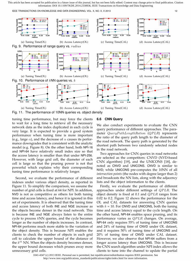
We also conduct experiments to evaluate the CNNquery performance of different approaches. The para-meter QueryPathLengthRation (QPLR) representsthe ratio of the query path length to the diameter ofthe road network. The query path is generated by theshortest path between two randomly selected nodesin the road network.
Two approaches for CNN queries in road networksare selected as the competitors: CNVD (NVD-basedCNN algorithm) [19], and the UNICONS [18], de-noted as CNVD and UNICONS. CNVD is similar toNVD; while UNICONS pre-computes the 10NN of allintersection points (the nodes with degree larger than 2)and broadcasts the NN lists, along with the adjacencylists and the object information to the clients.
Firstly, we evaluate the performance of differentapproaches under different settings of QPLR. Theobject density is fixed at 0.1 and QPLR ranges from0.02 to 0.2. Figure 12 shows the performance for theOL and CAL datasets for answering CNN querieswith k = 10. For CNVD and UNICONS, both the tuningtime and access latency equal to the cycle length. Onthe other hand, NPI-64 enables space pruning, and itsperformance varies as QPLR changes. On average,NPI-64 only requires 55% of tuning time of UNICONSand 24% of tuning time of CNVD under OL dataset,and it requires 50% of tuning time of UNICONS and20% of tuning time of CNVD under CAL dataset.However, we also observe that NPI-64 suffers from alonger access latency than UNICONS. This is becausethe CNN search algorithm under NPI index allows theclients to tune into the channel to update the partial
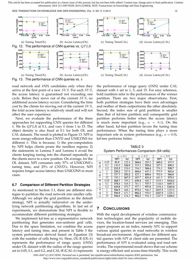
1041-4347 (c) 2013 IEEE. Personal use is permitted, but republication/redistribution requires IEEE permission. Seehttp://www.ieee.org/publications_standards/publications/rights/index.html for more information.
This article has been accepted for publication in a future issue of this journal, but has not been fully edited. Content may change prior to final publication. Citationinformation: DOI 10.1109/TKDE.2014.2330836, IEEE Transactions on Knowledge and Data Engineering
IEEE TRANSACTIONS ON KNOWLEDGE AND DATA ENGINEERING, VOL. X, NO. X, X 2013 13
0.01 0.05 0.10 0.15 0.20200
500
800
1100
1400
Tu
ning
Tim
e(KB
)
QPLR
NPI-64 NVD UNICONS
(a) Tuning Time(OL)
0.05 0.10 0.15 0.20400
750
1100
1450
Acce
ss L
aten
cy(K
B)
QPLR
NPI-64 NVD UNICONS
0.01
(b) Access Latency(OL)
0.05 0.10 0.15 0.20
1000
2000
3000
Tuni
ng T
ime(
KB)
QPLR
NPI-64 NVD UNICONS
0.01
(c) Tuning Time(CAL)
0.05 0.10 0.15 0.201100
1900
2700
3500
Acce
ss L
aten
cy(K
B)
QPLR
NPI-64 NVD UNICONS
0.01
(d) Access Latency(CAL)
Fig. 12. The performance of CNN queries vs. QPLR
1 5 10 15200
400
600
800
1000
1200
Tuni
ng T
ime(
KB)
k
NPI-64 NVD UNICONS
(a) Tuning Time(OL)
5 10 15400
600
800
1000
1200
Acce
ss L
aten
cy(K
B)
k
NPI-64 NVD UNICONS
1
(b) Access Latency(OL)
5 10 15500
1300
2100
2900
3700
Tuni
ng T
ime(
KB)
k
NPI-64 NVD UNICONS
1
(c) Tuning Time(CAL)
5 10 151000
1500
2000
2500
3000
3500
Acce
ss L
aten
cy(K
B)
k
NPI-64 NVD UNICONS
1
(d) Access Latency(CAL)
Fig. 13. The performance of CNN queries vs. k
road network and kNN candidates only when theyarrive at the first point of a new SV S. For each SV S,the access latency is guaranteed not exceeding onecycle. Before they move out of the current SV S, noadditional access latency occurs. Considering the timecost by the clients for moving out of the current SV S,the total access latency is relatively small and will notaffect the user experience.
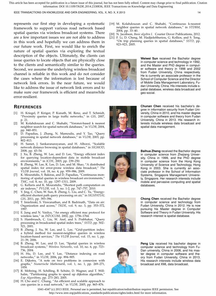
Next, we evaluate the performance of the threeapproaches for supporting CNN queries for differentk. We fix QPLR at 0.1, and vary k from 1 to 15. Theobject density is also fixed at 0.1 for both OL andCAL datasets. The result is plotted in Figure 13. NPI ismore energy-efficient than CNVD and UNICONS fordifferent k. This is because; 1) the pre-computationby NPI helps clients prune the needless regions; 2)the statements in Lemma 5 and Lemma 6 avoid theclients keeping tuning into the channel repeatedly asthe clients move to a new position. On average, for theOL dataset, NPI consumes only 57% of UNICONS’stuning time, and 25% of CNVD’s. However, NPIrequires longer access latency than UNICONS in mostcases.
6.7 Comparison of Different Partition Strategies
As mentioned in Section 3.1, there are different stra-tegies to partition the road network into smaller cells.Although we adopt the grid partition as the defaultstrategy, NPI is actually independent on the under-lying network partitioning algorithms. In last set ofexperiments, we demonstrate that NPI is flexible toaccommodate different partitioning strategies.
We implement kd-tree as a representative networkpartitioning that generates non-uniform grid cells.Due to the space limitation, we combine the accesslatency and tuning time, and present in Table 3 thesystem performance derived based on Equation (3)with the number of cells being 64. Here, OL-R (OL-k)represents the performance of range query (kNN)under OL dataset with the radius of the range queriesset to 0.05, 0.1, and 0.2, and CAL-R (CAL-k) represents
the performance of range query (kNN) under CALdataset with k set to 1, 5, and 15. For easy reference,bold numbers refer to the performances of the winnerpartition. There are two major observations. First,both partition strategies have their own advantagesand neither of them outperforms the other absolutely.Second, the index size of grid partition is smallerthan that of kd-tree partition and consequently gridpartition performs better when the access latencyis much more important (e.g., α = 0.1). On theother hand, kd-tree partition favors the tuning timeperformance. When the tuning time plays a moreimportant role in system performance (e.g., α = 0.9),kd-tree performs better.
TABLE 3System Performances Comparison (64 cells)
α = 0.1 α = 0.5 α = 0.9NPI kd NPI kd NPI kd
OL-
R 0.05 91.9 122.4 268.6 289.2 445.2 455.90.1 130.9 126.9 319.3 292.6 507.6 458.10.2 212.5 218.0 394.3 384.4 576.2 550.7
OL-k 1 229.2 247.8 404.6 405.2 579.9 562.6
5 257.3 253.2 425.1 409.6 592.8 566.015 330.1 267.5 485.7 421.4 641.3 575.3
CA
L-R 0.05 260.7 359.2 639.4 686.7 1018.1 1014.2
0.1 378.3 418.3 761.1 737.7 1144.0 1057.10.2 619.8 670.7 957.1 957.0 1294.4 1243.4
CA
L-k 1 526.9 668.1 872.2 946.5 1217.5 1225.0
5 536.9 671.7 882.2 950.0 1227.5 1228.215 556.9 674.3 902.2 952.3 1247.5 1230.3
7 CONCLUSIONS
With the rapid development of wireless communica-tion technologies and the popularity of mobile de-vices, the location-based services are emerging. Thispaper proposes an air index, namely NPI, to supportvarious spatial queries in road networks in wirelessbroadcast environment. Algorithms for different spa-tial queries with NPI at client side are presented. Theperformance of NPI is evaluated using real road net-works. The experimental result shows that our schemeis energy-efficient and access-time-friendly. This work
1041-4347 (c) 2013 IEEE. Personal use is permitted, but republication/redistribution requires IEEE permission. Seehttp://www.ieee.org/publications_standards/publications/rights/index.html for more information.
This article has been accepted for publication in a future issue of this journal, but has not been fully edited. Content may change prior to final publication. Citationinformation: DOI 10.1109/TKDE.2014.2330836, IEEE Transactions on Knowledge and Data Engineering
IEEE TRANSACTIONS ON KNOWLEDGE AND DATA ENGINEERING, VOL. X, NO. X, X 2013 14
represents our first step in developing a systematicframework to support various road network basedspatial queries via wireless broadcast systems. Thereare a few important issues we are not able to addressin this work and hopefully we can address them inour future work. First, we would like to enrich thenature of spatial queries via exploring the textualdescription of the objects. Ultimately, the clients canissue queries to locate objects that are physically closeto the clients and semantically similar to the queries.Second, we assume the underlying wireless broadcastchannel is reliable in this work and do not considerthe cases where the information is lost because ofnetwork link errors. In the near future, we wouldlike to address the issue of network link errors and tomake sure our framework is efficient and meanwhileerror-resilient.
REFERENCES[1] H. Kriegel, P. Kroger, P. Kunath, M. Renz, and T. Schmidt,
“Proximity queries in large traffic networks,” in GIS, 2007,p. 21.
[2] M. Kolahdouzan and C. Shahabi, “Voronoi-based k nearestneighbor search for spatial network databases,” in VLDB, 2004,pp. 840–851.
[3] D. Papadias, J. Zhang, N. Mamoulis, and Y. Tao, “Queryprocessing in spatial network databases,” in VLDB, 2003, pp.802–813.
[4] H. Samet, J. Sankaranarayanan, and H. Alborzi, “Scalablenetwork distance browsing in spatial databases,” in SIGMOD,2008, pp. 43–54.
[5] J. Xu, B. Zheng, W. Lee, and D. Lee, “Energy efficient indexfor querying location-dependent data in mobile broadcastenvironments,” in ICDE, 2003, pp. 239–250.
[6] B. Zheng, W. Lee, K. Lee, D. Lee, and M. Shao, “A distributedspatial index for error-prone wireless data broadcast,” TheVLDB Journal, vol. 18, no. 4, pp. 959–986, 2009.
[7] K. Mouratidis, S. Bakiras, and D. Papadias, “Continuous mon-itoring of spatial queries in wireless broadcast environments,”TMC, vol. 8, no. 10, pp. 1297–1311, 2009.
[8] G. Kellaris and K. Mouratidis, “Shortest path computation onair indexes,” PVLDB, vol. 3, no. 1-2, pp. 747–757, 2010.
[9] Y. Jing, C. Chen, W. Sun, B. Zheng, L. Liu, and C. Tu, “Energy-efficient shortest path query processing on air,” in SIGSPATIALGIS, 2011, pp. 393–396.
[10] T. Imielinski, S. Viswanathan, and B. Badrinath, “Data on air:Organization and access,” TKDE, vol. 9, no. 3, pp. 353–372,1997.
[11] E. Jung and N. Vaidya, “An energy efficient mac protocol forwireless lans,” in INFOCOM, 2002, pp. 1756–1764.
[12] S. Hambrusch, C. Liu, W. Aref, and S. Prabhakar, “Queryprocessing in broadcasted spatial index trees,” SSTD, pp. 502–521, 2001.
[13] B. Zheng, J. Xu, W. Lee, and L. Lee, “Grid-partition index:a hybrid method for nearest-neighbor queries in wirelesslocation-based services,” The VLDB Journal, vol. 15, no. 1, pp.21–39, 2006.
[14] B. Zheng, W. Lee, and D. Lee, “Spatial queries in wirelessbroadcast systems,” Wireless Networks, vol. 10, no. 6, pp. 723–736, 2004.
[15] H. Hu, D. Lee, and V. Lee, “Distance indexing on roadnetworks,” in VLDB, 2006, pp. 894–905.
[16] E. Dijkstra, “A note on two problems in connexion withgraphs,” Numerische Mathematik, vol. 1, no. 1, pp. 269–271,1959.
[17] R. Mohring, H. Schilling, B. Schutz, D. Wagner, and T. Will-halm, “Partitioning graphs to speed up dijkstras algorithm,”Exp Algorithms, pp. 273–283, 2005.
[18] H. Cho and C. Chung, “An efficient and scalable approach tocnn queries in a road network,” in VLDB, 2005, pp. 865–876.
[19] M. Kolahdouzan and C. Shahabi, “Continuous k-nearestneighbor queries in spatial network databases,” in STDBM,2004, pp. 33–40.
[20] N. Jacobson, Basic algebra I. Courier Dover Publications, 2012.[21] F. Li, D. Cheng, M. Hadjieleftheriou, G. Kollios, and S. Teng,
“On trip planning queries in spatial databases,” SSTD, pp.923–923, 2005.
Weiwei Sun received the Bachelor degreein computer science and technology in 1992,and the Master and PhD degree in comput-er software and theory in 1998 and 2002from Fudan University, China respectively.He is currently an associate professor in theSchool of Computer Science and the Directorof Mobile Data Management Laboratory, Fu-dan University, China. His interests include s-patial database, wireless data broadcast andgeo-social.
Chunan Chen received his bachelor’s de-gree in information security from Fudan Uni-versity, China in 2010, and his master degreein computer software and theory from FudanUniversity, China in 2013. His research in-terests include wireless data broadcast andspatial data management.
Baihua Zheng received the Bachelor degreein computer science from Zhejiang Univer-sity, China in 1999, and the PhD degreein computer science from the Hong KongUniversity of Science and Technology, HongKong in 2003. She is currently an asso-ciate professor in the School of InformationSystems, Singapore Management Universi-ty, Singapore. Her research interests includemobile and pervasive computing and spatialdatabases.
Chong Chen received the Bachelor degreein computer science and technology fromFudan University, China in 2012. He is nowpursuing his Master degree in ComputerSoftware and Theory in Fudan University. Hisresearch interest is spatial database.
Peng Liu received his bachelor degree incomputer science and technology from Fu-Dan university, China in 2008, and his mas-ter degree in computer software and the-ory from Fudan University, China in 2013.His research interests include wireless databroadcast and XML data broadcast.


