1

Since the introductory lecture was some time ago, and we only scratched the surface of plasticity, we want to recall fundamental phenomena of plasticity that will be essential in the following. Those are the ingredients of the general or classical plasticity theory. We can summarize them basically in the pictures on this slide. We have linear elastic behavior up to the yield point. From there on plastic strains will evolve. This point is not the same everywhere in the material, so not all material points will start to flow simultaneously. Hence we do not have a sharp transition from elastic to plastic, but a rather smooth transition with micro‐plasticity up to macro plasticity. However, if we stop at some time, like the point B and unload the material, we will elastically unload with a modulus parallel to the initial one, at least for many metals. When completely unloaded we realize a permanent strain or plastic strain that has developed so far until reaching the point B. The observed strain in point B was hence the sum of the permanent plastic stain and the elastic one. Upon reloading we move back on the same line until reaching point B, from were on plasticity sets back in – in an ideal case. The value sigma_B is called the subsequent yield stress, that can strongly differ from the initial one.

If we reverse the load, we observe that the subsequent reversed yield stress in opposite direction is much less than the negative subsequent one. We learned that this is called Bauschinger effect, that describes the directional dependence or anisotropy of the yield stress after plastic deformation. Do you remember why?

The effect can be explained by the summation and inter blocking of dislocations in the material. The microscopic stress distribution inside the material due to its past determines this behavior. By plastic deformation, many dislocations are accumulated at 

2

dislocation barriers like grain boundaries, resulting in hardening. Now if one inverts the loading direction, the following happens:1. Local reaction stress to the accumulated dislocations promotes dislocation movements 

in the opposite direction. Hence dislocations can move backwards easier, lowering the yield stress.

2. When the deformation direction is inverted, dislocations with opposite sign can be emitted from the same source, cancelling out the initially emitted ones. Since the dislocation density decreases, the yield stress decreases as well.

2

Most of the phenomena in elasto‐plastic material behavior can already be studied in the uni‐axial case.

3

4

To describe the non‐linear relation between stress and strain in particular for metals with strain hardening in the plastic regime, simple functions can be used to fit experimental curves. First we will look at models that use absolute properties.

The Ramberg‐Osgood curve is such an example that is quite popular. In principle one has an elastic part (left term) and a plastic one (right term) that can be fitted in terms of magnitude and importance by the parameters K and n. In the simplest form already hardening occurs below the yield limit. To weaken this effect, the yield stress sigma_0 can be used along with the new parameter alpha. This value can be fitted to the 0,2% plastic strain value alpha*sigma_0/E=0.002. Often just a simple value for alpha=3/7 is taken, what corresponds to the experience, that the secant modulus E/(1+alpha)= E*7/10. The exponent n has for metals values around 5 or larger. As on can observe the value n=inf corresponds to ideal elastic‐plastic behavior, hence a horizontal line starting at the yield stress.

5

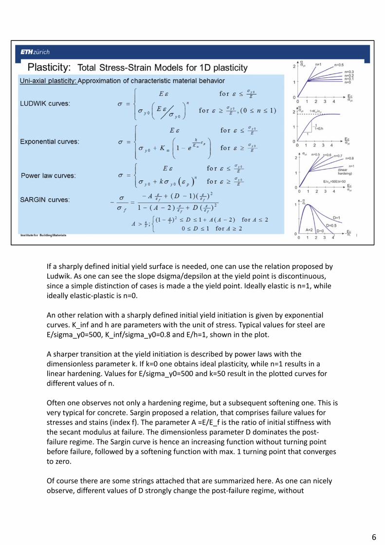
If a sharply defined initial yield surface is needed, one can use the relation proposed by Ludwik. As one can see the slope dsigma/depsilon at the yield point is discontinuous, since a simple distinction of cases is made a the yield point. Ideally elastic is n=1, while ideally elastic‐plastic is n=0.

An other relation with a sharply defined initial yield initiation is given by exponential curves. K_inf and h are parameters with the unit of stress. Typical values for steel are E/sigma_y0=500, K_inf/sigma_y0=0.8 and E/h=1, shown in the plot.

A sharper transition at the yield initiation is described by power laws with the dimensionless parameter k. If k=0 one obtains ideal plasticity, while n=1 results in a linear hardening. Values for E/sigma_y0=500 and k=50 result in the plotted curves for different values of n.

Often one observes not only a hardening regime, but a subsequent softening one. This is very typical for concrete. Sargin proposed a relation, that comprises failure values for stresses and stains (index f). The parameter A =E/E_f is the ratio of initial stiffness with the secant modulus at failure. The dimensionless parameter D dominates the post‐failure regime. The Sargin curve is hence an increasing function without turning point before failure, followed by a softening function with max. 1 turning point that converges to zero.

Of course there are some strings attached that are summarized here. As one can nicely observe, different values of D strongly change the post‐failure regime, without 

6

influencing the pre‐failure regime.

As one can easily imagine a large number of other functional approximations can be made for uni‐axial plasticity. However for now we want to take a track, that has the potential to go to 3D.

6

Models with total properties miss the possibility to consider the loading history e.g. for cyclic loading, if we just think of the Bauschinger effect. Hence one can only use such models for problems under monotonic loading, for unloading or reloading incremental formulations are needed. In principle one could also use hypo elastic concepts, that we had a look at for non‐linear elastic laws, however that would be much more complicated than incremental plasticity theory. Once we did the 1D case, we can extend it to 3D plasticity. For an incremental formulation we need 5 steps: Loading type, flow rule, hardening rule, hardening parameters and the consistency condition. 3‐4 are of course insignificant of ideally plastic behavior.

The loading type is identified via the yield function or loading function f. In 3D f is defined as the yield surface in stress space. In principle we can always change into the elastic domain by changing in the loading direction. Simplified, we have 2 different regimes, a plastic and an elastic one. If a stress increment dsigma leads into the plastic domain, the system is loaded, otherwise it is unloaded. Let’s have a look at the loading function f. If the yield stress in compression and tension is k, one can write sigma^2‐k^2. If f=0, we are in the plastic regime. If df<0 the material point is elastically unloaded, df>0 means plastic deformation and the case df=0 is called neutral loading. There is a large number of loading functions that are all formulated in the stress space for practical reasons.

7

If the stress state sigma is incremented with dsigma, this results in a stress state sigma+dsigma outside of the elastic domain. The sign of the resulting plastic strain increment depsilon_p has the same sign as dsigma. Depsilonp can hence be considered as vector in the plastic strain space that is superposed to the stress space in the figure. It points outwards at the yield point and is expressed by…., with dlamda, a non‐negative scalar. This relation is called flow rule. If the flow rule comprehends the loading function f, one talks of an associated flow row, if a different type is used it is a non‐associated flow rule. Note that the flow rule gives the sign of the plastic strain increment but not its magnitude (lambda).

By plastic deformation, the position or size of the elastic domain changes. The lower and upper yield stress is thus a consequence of the loading history or more precisely only of its plastic part, since elastic deformations have no influence on yield stresses. The deformation history hence has to be recorded correctly to be able to determine the present state of a material element correctly. Hardening rules are an important part of plasticity formulations. Those are models that have to realistically predict, how the yield surfaces evolve depending on the plastic deformation history. The two simplest and extreme approaches are kinematic and isotropic hardening. Often mixed criteria are used that comprise both approaches. In principle one does not formulate the yield surface only as functions of some invariants, but also as function of the hardening parameters. The hardening parameters characterize the way, how the subsequent yield surface evolved in position and shape upon plastic deformation.

For kinematic hardening the size of the elastic domain remains unchanged. For the 

8

initial yield strength sigma_0 yield sets in under compression, if sigma=sigma_t ‐2*sigma_0. The yield surface behaves like an undeformed body, that is translated in stress space whenever a plastic deformation occurs. This is made via the back stress tensor alpha, that stores the plastic deformation. Kinematic hardening can represent the Bauschinger effect.

For isotropic hardening the main assumption is that hardening under tension results in an equally large hardening as under compression and vice versa. The yield surface is thus isotropic extended. This is described by the hardening function k that scales the size of the elastic domain. Consequently no Bauschinger effect can be represented in isotropic hardening. Note that mechanisms resemble extreme cases that can be combined via mixing parameters.

8

Since yield stresses depend on the past plastic deformations (except for ideal plasticity), also multi‐dimensional yield surfaces change. Here we look at the biaxial case for visualization purposes. Before plastic deformation sets in, all Ks=0 and just the initial yield surface exists. The choice of hardening parameters hence determines the choice of hardening rules. The parameters are not constant, but depend on the plastic deformation state, e.g. the values of the internal variables of the plastic strain tensor epsilon_ij^p or on the so called plastic work W_p – two different ways to memorized the plastic deformations. One also call these internal variables also state variables, that we can call kappa_beta. 3D is not different, just more difficult to visualize.

9

As we already know, we have to record the plastic loading history. For this purpose scalar hardening parameters are used. In principle their number is not limited, for practical reasons however only one hardening parameter is used. We want to focus on two parameters, the effective plastic strain and the plastic work.

The effective plastic strain can be seen as a summation of all plastic strains and its magnitude never decreases. This way the entire plastic loading history is recorded. The second hardening parameter is called plastic work Wp, what is nothing but the dissipated energy by plastic deformation. The hardening behavior is consequently called strain or work hardening, and one can write the evolution function kappa for isotropic hardening with the hardening parameters kappa. The back stress tensor is consequently also a function of the plastic loading history. Since alpha can fluctuate, depending on the loading direction, it has to be expressed in incremental form. Sigma_e is the effective stress, that shows how the stress fluctuates in the loading history.

10

The condition that during plastic deformation the stress state always remains on the edge of the elastic domain is called consistency condition. In other word, the elastic domain has to change so the current stress state can remain on the yield surface if the material deforms elastic‐plastic. Mathematically this is written….

Now the 5 steps are complete and we repeat:

11

The incremental strain can be decomposed into elastic and plastic part. Of course onlyupon loading there is a chance for a plastic increment. If we insert the flow rule, the consistency condition and hardening rule, we obtain an expression for the scalar dLambda, the magnitude of the plastic strain increment. In a brief way with the tangent modulus E_t it can be expressed :….. Inside the tangent modulus now the entire deformation history is stored.

12

We can also alternatively derive this and obtain the reciprocal tangent modulus. 

If now epsilon_p is the hardening parameter, we obtain depending on the hardening rule (kinematic or isotropic)…. The terms dsigma_e/dkappa and dk/depsilon_p capture how the stresses during plastic deformation change and can be experimentally measured. It is called plastic modulus E_P. Hence one can write for the three moduli…

13

14

Plastic deformations of materials are defined via yield surfaces. Those are 5 dimensional, convex surfaces in a 6 dimensional stress space. Mathematically yield criteria are formulated via yield surfaces f, whose size, shape and position can change by hardening processes, as we already know. The original form is called initial yield surface, all other ones are called subsequent yield surfaces. All points inside correspond to elastic while the ones on the surface result in yielding. We already looked at failure surfaces, however for plasticity it is the same, only the interpretation is different. If the load is further increased no points outside the surface are taken, but the surface evolves.

Yield surfaces are formulated in diverse stress spaces. The most common one is the Cauchy principle stress space. Other ones are….

Note that for anisotropic materials orientations of principal stresses are important and yield surfaces should not be expressed in invariants.

The most common way to classify criteria is by the way hydrostatics stresses act: if independent (non‐frictional like metals) and those where hydrostatic stresses are important called frictional materials. Isotropic yield surfaces or multiple surfaces are other cases. Let’s have a deeper look.

15

This we know already. Theta is again the Lode angle with 0<theta<60°. As we can see I1 is nowhere to be found. For vonMises also I3 is absent and hence the Lode angle. This is the fundament of J2‐plasticity.

The HOSFORD criterion resembles a function that can be used to combine vonMises with Tresca by a parameter n. It is thus a generalization of the vonMises criterion.

16

This we also know. The Rankine criterion for brittle tensile failure. The surface is often used as tension‐cutoff and one nicely sees the I1 dependence.The MC has as addition to the Tresca criterion the dependence on sigma, while the DP can seen as extension of the vonMises with I1 dependence. One can express the DP by c and phi as well. If the compressive median is taken the DP encloses the MC (+), while with the tensile median the MC encloses the DP (‐).Of course we could continue now with the BRESLER PISTER criterion (extension of DP), the WILLAM WARNKE criterion or the 7 parameter BIOGONI PICCOLROAZ criterion, just to name a few, but those are very material specific yield surfaces. What we could however look at is how anisotropy is considered.

17

18

The LOGAN‐HOSFORD yield criterion is in principle a generalized vonMises criterion with scaling in the principal axes. Since the principle directions have to be coaxial with the material coordinates, it only work for crystal lattices.

The Hills yield criterion is much more general and in its original form in principle also only a scaled variant of the vonMises criterion. An improved version for generalization comes with an exponent m. Variations of the criterion are often used for metals, polymers and certain composites. One needs 6 yield stresses: 3 normal yield stresses with respect to anisotropy axes and three shear yield stresses.

If the principal axes coincide with the orientation of the material coordinate system, one can use a generalized form of the criterion with exponent m, that is giving the anisotropy of the material and has to be >1 to assure convex surfaces for stability.

The initial yield surfaces are independent from pressures. Extensions, that consider this are CADDEL‐RAGHAVA‐ATKINS (CRA) or the DESHPOANDE‐FLECK‐ASHBY (DFA) yield criterion. The DFA criterion reminds of the BRESLER‐PISTER criterion and is used for honeycombs. Of course from all criteria, version for plane stress and strain exist.

19

In the 50s and 60s huge progress was made in classical plasticity theory driven by Drucker:

The theory of the limit analysis lead to a practical method for assessing the loading capacity of structures. The concept of material stability brought a unified perspective of stress‐strain relations for plastic bodies, while the idea of the normality condition made the required connection between yield criterion or loading function to the plastic stress‐strain relation. These developments were the foundation of the classical plasticity theory and starting point for many further developments e.g. for concrete or soil plasticity. We develop here the plastic stress‐strain relations for perfect plasticity and work hardening materials. Of course in the framework of incremental plasticity, that we already elaborated for 1D and are now about to extend to 3D. Upon completion we will have a comprehensive description of stress‐history dependent behavior of plastic bodies.

The yield function=loading function defines the limit of the elastic domain in the stress space. In internal point (f<0) resembles purely elastic behavior, while all points on the surface (f=0) resemble plastic behavior. Points outside are not allowed, as we know. If we are sitting just on the surface, it is important to know, if the load increment points inwards (unloading), tangential (neutral loading) or outwards (loading) what corresponds to a material classification. The plastic deformations result at least for hardening materials in a modification of the yield surface to assure, that the stress state remains on the subsequent yield surface. Yield surfaces always have to be defined in a way, that their gradient df/dsigma_ij = n_ij^f always points outwards and is the outward 

20

pointing normal vector of the surface (f=0). This is visualized in the image. For ideally plastic materials the loading case and neutral loading is identical. Instead of stress increments, also strain increments can be used to decide on the loading type. For FE, the strain increment approach is more convenient, since stresses have to be calculated with extra effort.

20

After the initiation of plasticity, the constitutive elastic equations render invalid. Plastic strains depend on the overall loading history of the material. The stress-strain relations are given in terms of strain increments. After decomposition of the strain increment into elastic and plastic part, for the plastic increment the direction and magnitude of the strain increment vector has to be calculated. This job is done with the flow rule, that contains the plastic potential function g. If g is of the same type as the yield surface we talk about associated flow rules, if a different function is used, it is non-associated. For metals associated flow rules work great, while frictional materials typically need non-associated flow rules. The flow rule gives the sign of the plastic strain increment and the gradient vector gives the direction. Note that the df/dsigma is the normal on the potential surface g=0 at the actual stress state. This is why the flow rule is also called normality condition. The magnitude of the plastic strain increment vector remains unknown and is called dlambda, a non-negative scalar function that of course will change during the loading history.

If the plastic potential is of vonMises (cylinder) type, on can see that the plastic strain increment tensor is in principle the scaled deviatoric stress tensor, hence principal directions coincide. Since no plastic dilatations occur, depsilon_kk=s_kk*dlampbda=0. The resulting relations are called Prandtl‐Reussequations and represent the flow rule for an ideally elastic‐plastic material. They give the relation between a plastic strain increment and the present stress deviator, but do not specify the magnitude of the strain increment. If the strain is quite large, the elastic increment becomes meaningless with respect to the total strain and the PRANDTL‐

21

REUSS equations become the LEVY‐MISES equations.

If the plastic potential is of TRESCA (hexagonal prism) type, using the principle stresses one can write….. As we can see, the strain increments perpendicular on the surface (AB) are always parallel. One problem is the case when two principal stresses are identical, what means the stress state is directly located on an edge and we have two possibilities for the normal direction. A work around consists in making a linear combination of the two vectors like…. This linear combination is in principle also applicable to other cases where surfaces are not continuously differentiable like multi‐surface plasticity. A different approach consists in behaving at the singularity as if one would have a vonMises yield surface in these points.

21

The loading function for ideally plastic materials demand, that the stress increment vector dsigma is tangential to the yield surface, while the flow rule demands that the vector of the plastic strain increment is normal to the plastic potential surface. What needs to be done is the determination of the magnitude of depsilon, in other words dlambda. If dlambda is calculated, the incremental stress‐strain relation is defined.

The total strain increment is composed of the elastic and plastic increment. The elastic one is defined via the Hook’s law and the plastic one via the flow rule, giving a constitutive relation with the yet unknown positive scalar dlambda. With the consistency condition, that the stress state remains on the yield surface, we obtain by inserting the stress‐strain relation the formulation for dlambda with the term H. This relation tells us, that not necessarily all stress increments that move on the yield surface produce plastic strains, as long as df/dsig*C*deps=0. This is neutral loading! In principle we can now calculate the stress increment for a given strain increment by inserting dlambda. What follow are some mathematical manipulations….

Since part_f/part_sigma is independent from dsigma and depsilon, the elastic‐plastic stiffness tensor represents a scalar that is used to scale the strain increment to obtain the corresponding stress increment. However the other way around does not work, as we can see on a simple one‐dimensional case.

22

Elastic‐ideally plastic stress‐strain relations, based on the von Mises yield criterion are called Prandtl‐Reuss material model. We have the yield surface f, potential surface g and yield constant k. J2 is most likely the most applied engineering model in plasticity and the most simple elastic‐ideally plastic material model. By inserting the yield surface into the elastic‐plastic relation, one obtains with the Lames constants….

We can write the constitutive relation in matrix form with the bulk and shear modulus. The inverse of C^ep does not exits (it is singular). For dlamba we can insert and obtain…. As we can see the plastic strain increment depends on the actual value of the stress but not on the increment needed to reach a new state. We can also write the increment of the plastic work…. The actual magnitude of the plastic strain increment dlambda, depends also directly on the actual increment of the plastic deformation work.

23

24

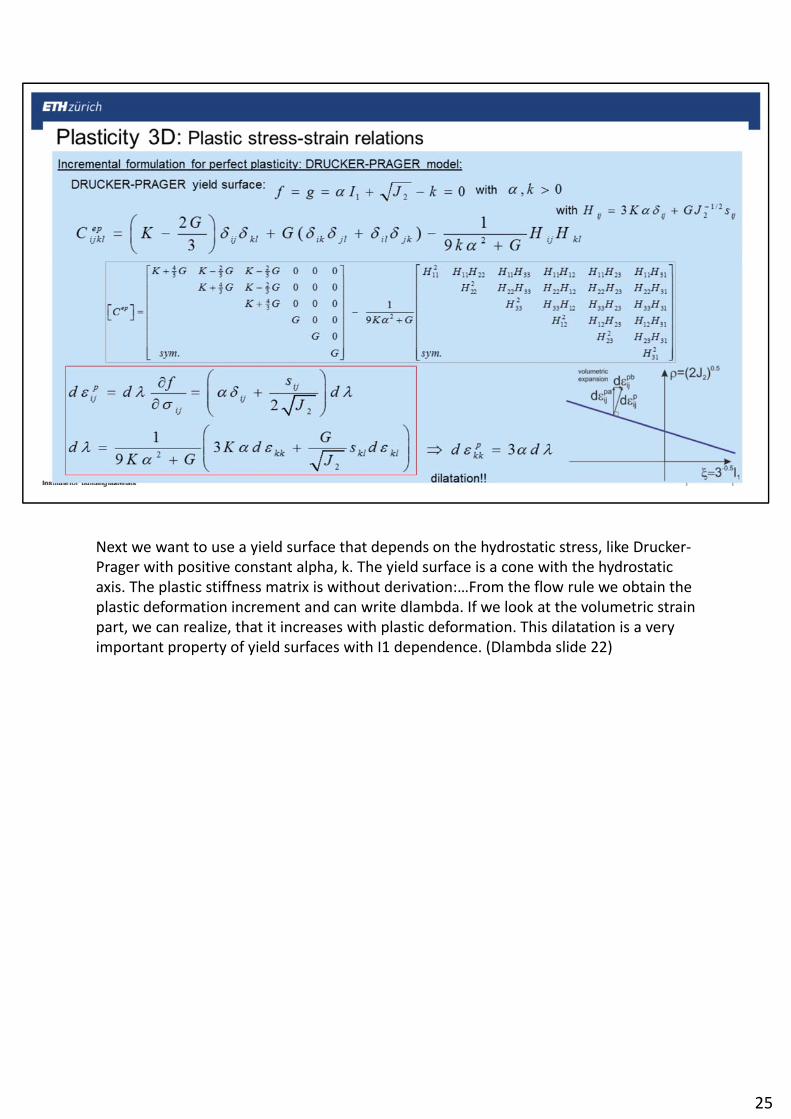
Next we want to use a yield surface that depends on the hydrostatic stress, like Drucker‐Prager with positive constant alpha, k. The yield surface is a cone with the hydrostatic axis. The plastic stiffness matrix is without derivation:…From the flow rule we obtain the plastic deformation increment and can write dlambda. If we look at the volumetric strain part, we can realize, that it increases with plastic deformation. This dilatation is a very important property of yield surfaces with I1 dependence. (Dlambda slide 22)

25

Top left: Pranl Ruess J2; top right DP with small strains; bottom DP with large strains

26

The flow rule, also called normality rule in principle comes from the requirement of irreversibility of the plastic deformation. This leads to limitations for the shape of the yield surface and finally also the uniqueness of the solution. Imagine a volume that is inside of the yield surface at sigma*. Now we move inside of the surface from A to B and C. C is located on the yield surface and we stay there for some time, what corresponds to sigma. Now plastic yield occurs and only plastic work is done. After a while we unload and go back via D and E to sigma*. Since the elastic deformation is reversible, the entire energy fro EBCDEA is recovered. The plastic work is the scalar product of the stress vectors sigma‐sigma* and of the plastic strain increment.  Because of the irreversible character of the plastic deformation, the plastic work is positive….. The scalar product between the vectors is then positive (image) if convexity and normality is fulfilled. The normality automatically results in associated flow with the gradient df/dsigma (normal vector) of the yield surface. Dlamda is consequently always positive and scalar to get positive plastic work.

27

As we already touched several times, yield surfaces evolve during load history, to enable stress states to be always located on their surface. The evolution is governed by the hardening rules. Isotropic hardening is an affine expansion of the yield surface without distortion or translation. It is described via the hardening parameter kappa. Kappa hence gives the size of the surface and is thus a property for the plastic loading history.

For kinematic hardening the yield surface moves in space like a rigid body without rotation. Size, shape and orientation are fixed. This model was proposed by Prager to be able to consider the Bauschinger effect. The formulation of the yield surface includes a back stress vector alpha, that moves the center of the body. Alpha varies with the loading history. How the incremental alpha is formulated is not fixed. Prager proposed a simple version of the back stress vector, that is a scaled version of the plastic strain increment vector with the scaling constant c. Hence the yield surface would always move normal to the subsequent yield surface. Ziegler proposed an other rule based on the Prager flow rule by moving the yield surface in the direction of the reduces stress tensor simga‐alpha. Dmü is a positive proportionality factor that depends on the deformation history, hence on a positive, material dependent scalar a that can be a function of the state variable kappa.

Of course both approaches can be combined in mixed hardening rules. M denotes the mixing parameter 0<M<1 with the extreme values for isotropic and kinematic hardening.

28

29

To describe the hardening behavior, we need the recording of the past plastic history as well as the dependence of the hardening from it. Just like we saw the growth function k for yield surfaces being described by the hardening parameters (state variable) kappa. This functional dependence changes with the material. Most often uni‐axial tests are made to determine the hardening parameters. For this loading case also the effective stress and effective plastic stains are defined. The hardening function k can only depend on the effective properties or kappa.

The effective plastic stress is defined as: ….. With A and n determined under uniaxial loading. For vonMises material this is shown here and one can express the hardening function directly as function of the effective stress. 

Up to now we saw two different hypotheses for the history recording: (1) work hardening, where the hardening depends on the total plastic work Wp and (2) strain hardening, where hardening depends on the effective plastic deformation. Also materials are classified by being either work or strain hardening types. Both parameters Wp and ep can be used as hardening parameters (=kappa). For practical reasons it is simpler to use ep. Ep is defined as… and is always positive and increasing. The constant c is defined such that for uniaxial load dep goes to de11p.The relation of the effective plastic strain to the effective stress characterizes the hardening behavior. We want to calibrate this at a uniaxial experiment. The ratio dsigma/depsilon =H_p is called plastic modulus. For isotropic hardening Hp represents the expansion rate. For mixed hardening the variation of sigma_e results in expansion and translation of the yield surface, what works a little bit different.

30

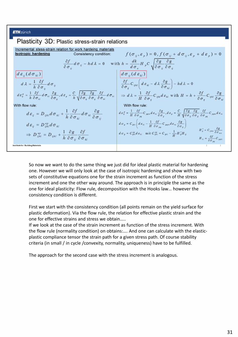
So now we want to do the same thing we just did for ideal plastic material for hardening one. However we will only look at the case of isotropic hardening and show with two sets of constitutive equations one for the strain increment as function of the stress increment and one the other way around. The approach is in principle the same as the one for ideal plasticity: Flow rule, decomposition with the Hooks law… however the consistency condition is different.

First we start with the consistency condition (all points remain on the yield surface for plastic deformation). Via the flow rule, the relation for effective plastic strain and the one for effective strains and stress we obtain…..If we look at the case of the strain increment as function of the stress increment. With the flow rule (normality condition) on obtains:…. And one can calculate with the elastic‐plastic compliance tensor the strain path for a given stress path. Of course stability criteria (in small / in cycle /convexity, normality, uniqueness) have to be fulfilled.

The approach for the second case with the stress increment is analogous.

31

32

Let’s summarize again the basic features of plastic metal behavior….

If we load a piece of metal uniaxial, we pass several states like the proportionality limit sigma_p, the elasticity limit sigma_e and finally the yield stress sigma_y. It can be determined either via the offset method, e.g. an offset of 0.2% plastic strain, or via the tangent method. In practice these three yield values are combined and one considers the behavior up to this point to be linear. After yielding one defines the tangent modulus (strain‐hardening Module E’<<E0). From here on the stress‐strain relation depends on history. 

33

34

Since metals are insensitive to hydrostatic stress, yield surfaces without I1 dependence are used (non‐frictional).

Of course there are again all possible invariant spaces you can think of to formulate the criteria. The vonMises criterion or distortion energy criterion is called in plasticity theory J2 theory or octahedral shear criterion. Sigma_y is the yield stress for uniaxial loading.

The loading function, surface or subsequent yield surface depend on the stress state, the state of the plastic deformation and its history k. For metals hardening parameters are often functions of the plastic trajectory or the total plastic work. However the hardening parameters can change depending on the metal and one uses three basic types: isotropic, kinematic and mixed. Kinematic hardening is also called anisotropic hardening model, since initially isotropic material becomes anisotropic by plastic deformation. Hence metals with Bauschinger effect have strong kinematic part, as well as metals under cyclic loading.

35

In principle there are two classical approaches for representing stress‐strain relations with metals and plastic deformations: The deformation and the yield theory. The fundamental assumptions are:

Deformation theory: For many engineering application the physical non‐linearity is more important than irreversibility and history dependence. Hencky (1925) proposed a simple deformation theory, that  is based on non‐linear elasticity theory. First the stress is decomposed into volumetric and deviatoric part. Since no volume changes are caused by the plastic deformation epsilon_kk=0. The second assumption results in the relation … with the scalar function theta, that expresses the material hardening. It is positive for loading and zero for unloading. In principle this way also the 1st assumption is included. Using the shear and bulk modulus, one can then obtain the strain state from the stress state. It is hence identical to non‐linear elastic stress‐strain relations with secant moduli – as long as the system is only loaded.

The flow theory or incremental theory we already looked at in detail. For the yield surface f only plastic deformation occurs if f=0 and we move always on the yield surface in a neutral loading  and so on.. The flow rule describes the interconnection between the next plastic strain increment at a stress state for a deformed material point. This relation reminds us of the stress‐strain relation for a viscos fluid and uses the principle of a plastic potential surface g. Dlambda is the positive scalar function, that depend on the state and history. If g=f we had associated flow. The direction of the plastic strain increment is always normal to the potential surface at the present stress state. (Normality condition). The magnitude of the plastic strain increment can be calculated 

36

with the assumption, that dlambda is proportion to the projection of the stress increment on the normal direction n_ij, hence n_ij*dsigma_ij. Consequently one can write for dlamda ….. With the hardening modulus H’, that depends on stress, strain and history.

36

The difference between deformation theory and Prandtl‐Reuss yield theory is in the incremental form of the stress‐strain relation. For this the total incremental stress‐strain relation can be derived. For the case of a very stiff, plastic material the elastic part becomes negligible and one obtains the LEVY‐MISES relation.

Prandtl‐Reuss implies the use of a vonMises yield surface with associated potential flow surface. In the general case this is not made. Starting from the linear, isotropic elastic relation multiplied with df/dsigma, we insert the plastic strain increment with associated flow. One makes some rearrangements and calculates for the plastic strain increment. In the following we will look at the hardening modulus H’ for perfect plasticity, isotropic, kinematic and mixed hardening.

37

For perfect plasticity this is simple, since the yield surface is fixed in space. Hence df=0 and H’=0 no hardening.

For isotropic hardening this is different. Here one assumes that the yield surface is isotropic and expanding without distortions, as soon as plastic deformations set in. The size of the yield surface is given by the hardening parameter k, that depends for strain hardening materials on the effective plastic strain and for work hardening ones on the total plastic work. The effective plastic strain depends on a constant parameter C, that depends on the used yield surface. For vonMises C=(2/3)^1/2.  From the consistency condition df=0 it follows: … Finally we insert the plastic strain increment and obtain the hardening modulus H’ for strain and work hardening materials.

38

For kinematic hardening one assumes, that the yield surfaces rigidly move in stress space. It has the form….. K is a constant and alpha_ij the coordinates of the center of the yield surface. Both change with the plastic deformation. Via consistency conditions we obtain a simple form for the hardening modulus. The type of hardening can be linear, called Prager's hardening rule. To obtain a kinematic hardening in stress space, Ziegler modified the Prager rule to obtain the movement rate of the yield surface in the direction of the reduced stress vector (sigma‐alpha) with positive, history dependent dmü. Dmü can have a simple form of a*depsilon_p what leads to….

For mixed hardening the Bauschinger effect can be considered to different amounts. With the consistency condition we obtain again the relation for the hardening modulus…

39

In principle most things are said. However one can express things in a more FE‐friendly version given here. One can write the incremental stress‐strain relation with the elastic‐plastic stiffness tensor. The hardening module can be expressed via the reduced stress tensor (dash), respectively in invariants. Mü and lambda are the Lame constants. In the most general form on gets….

40

Depending on the hardening rule the yield surfaces and hardening modules can be written…

41

Die konventionellen Plastizitätsmodelle sind einfach anzuwenden, beschreiben aber kompliziertere Belastungsgeschichten wie zyklische Plastizität nicht genau genug. Eine Erweiterung für diesen Fall ist das Grenzflächenmodell, das von Dafalias und Popov 1976 vorgeschlagen wurde. Das Modell findet bei Metallen oder bei Böden Anwendung.

Die Grundlage des Modells ist die Beobachtung der Veränderung des plastischen Moduls E_p=dsimga/depsilon_p. Eine typische dsigma‐depsilon_p Kurve ist hier gezeigt. Es gibt prinzipiell 3 unterschiedliche Regionen: (1) elastische Region mit unendlich hohem Ep. (2) nach Erreichen der Anfangsfliessspannung mit schneller Abnahme von Ep als Funktion der plastischen Dehnung. (3) konstanter Wert für Ep=E0, der mit der Begrenzungslinie XX’ assoziiert ist. Aus uniaxialen Versuchen zeigt sich, dass die Annahme einer Gerade für XX’ gerechtfertigt ist. Dieses Verhalten kann durch die dargestellte Gleichung als Funktion der beiden Parametern delta und delta_in [Pa] an einem bestimmten Punkt A1 ausgedrückt werden. Beide sind immer positiv. Delta ist der Abstand zwischen einen bestimmten plastischen Spannungszustand z.B. A1 und dem assoziierten Punkt auf der Grenzfläche A1balken bei gleicher plastischer Dehnung. Es ist also ein diskreter Geschichtsparameter. Delta_in ist der Anfangswert bei Fliessbegin. H ist ein Materialformparameter der experimentell bestimmt werden muss.

In 3D Spannungszuständen sind es natürlich keine Geraden sondern Flächen Grenzflächenmodell. Es gibt immer zwei Flächen, eine Grenzfläche und eine Belastungsfläche. Die Grenzfläche schliesst immer die Belastungsfläche ein. Alpha ist wieder die Lage des Zentrums der Belastungsfläche im Spannungsraum (Punkt K) und qnsind plastische innere Variablen (PIV) wie z.B. eine plastische Dehnung. Die 

42

Belastungsfläche kann sich natürlich unter beliebigen Verfestigungsregeln verschieben und verformen, wobei der Verfestigungsmodul H’ auch von delta abhängt. Die Grenzfläche beinhaltet den Vektor alpha* zum Zentrum des Körpers. Die Grenzfläche bewegt sich im Spannungsraum gemäss der Beziehung…. dalpha* ist das Translationsinkrement dalpha*. Dsigma/cos(omega)v_ij repräsentiert das Inkrement des Punkts A in Richtung des Einheitsvektors v_ij. Aufgrund der Bewegung der Belastungsfläche. H0’ ist der Verfestigungsmodul für Kontakt (delta=0), dsigma die Projektion des Spannungsinkremententensors auf den Normalenvektor n_ij und mü_ij ist der Einheitsvektor von A nach C. Wenn sich die Belatungsfläche lediglich starr verschiebt, wird der erste Term identisch zu dalpha_ij. Hier lässt sich jetzt wieder Pragers und Zieglers Verfestigungsregel verwenden, aber so weit wollen wir gar nicht gehen.

42

43