Surface plasticity: theory and computation

Computational Mechanics (2018) 62:617–634https://doi.org/10.1007/s00466-017-1517-x

ORIG INAL PAPER

Surface plasticity: theory and computation

A. Esmaeili1 · P. Steinmann1 · A. Javili2

Received: 12 July 2017 / Accepted: 14 November 2017 / Published online: 22 November 2017© Springer-Verlag GmbH Germany, part of Springer Nature 2017

AbstractSurfaces of solids behave differently from the bulk due to different atomic rearrangements and processes such as oxidationor aging. Such behavior can become markedly dominant at the nanoscale due to the large ratio of surface area to bulkvolume. The surface elasticity theory (Gurtin and Murdoch in Arch Ration Mech Anal 57(4):291–323, 1975) has provento be a powerful strategy to capture the size-dependent response of nano-materials. While the surface elasticity theory iswell-established to date, surface plasticity still remains elusive and poorly understood. The objective of this contributionis to establish a thermodynamically consistent surface elastoplasticity theory for finite deformations. A phenomenologicalisotropic plasticity model for the surface is developed based on the postulated elastoplastic multiplicative decomposition ofthe surface superficial deformation gradient. The non-linear governing equations and the weak forms thereof are derived. Thenumerical implementation is carried out using the finite element method and the consistent elastoplastic tangent of the surfacecontribution is derived. Finally, a series of numerical examples provide further insight into the problem and elucidate the keyfeatures of the proposed theory.

Keywords Surface elasticity · Surface plasticity · Finite element method

1 Introduction

The boundary of a continuum body can display its own dis-tinct properties compared to those of the bulk, e.g. due tobroken atomic bonds at the surface. This phenomenon isusuallymodeled via surface stresses [13,25,30,42,64] associ-ated with a zero-thickness layer on the material. The surfacestress can also be derived fromaboundary potentialwhen onedeals with a conservative formulation. Such surface poten-tial usually depends only on the surface deformation gradientand also on the surface normal in the case of anisotropy. Inaddition, the difference between the properties of the bound-ary of a continuum body and those of the bulk can also be

B A. [email protected]

A. [email protected]

P. [email protected]

1 Chair of Applied Mechanics, University ofErlangen–Nuremberg, Egerlandstrasse 5, 91058 Erlangen,Germany

2 Department of Mechanical Engineering, Bilkent University,06800 Ankara, Turkey

due to exposing the surface to processes such as oxidation,aging, grit blasting, plasma jet treatment, etc. Phenomeno-logical modeling of such surfaces is achieved by endowingthe surface with its own energy, and further surface specificthermodynamic ingredients, see [1,27,36–39,41,64,65].

In the context of the current work, due to some confusionin the literature, the definitions of the terms surface stress andsurface energy shall be re-iterated. Surface energy is usuallyunderstood as an excess energy term due to the presence ofthe surface as an enegetic layer or also as a superficial energyterm due to rearrangement of atoms very close to a surface[25,40]. Alternatively, one can regard the surface energy tobe associated with either the creation of a new surface atconstant strain or the deformation (straining) of the alreadyexisting surface [43], see also [23,57,58,67]. Surface stressis the force responsible for elastically deforming the surfaceof the body resulting in the change of the distances amongatoms or molecules on the surface [42].

In the current work, we build upon the surface elasticitytheory of Gurtin and Murdoch [30]. The surface elasticitytheory is a well-established methodology to capture the size-dependent behavior of materials at the nano-scale and hasbeen extensively studied in the past decades, see e.g. [5,7–9,12,28,31,36,44–47,50,56,63,66,69] and references therein.

123

http://crossmark.crossref.org/dialog/?doi=10.1007/s00466-017-1517-x&domain=pdf

618 Computational Mechanics (2018) 62:617–634

The effect of surface energetics, e.g. for inclusions, and thesize-dependent elastic state of the material has recently beeninvestigated for instance in [3,4,6,10,13–17,24,33,49,53–55,68] and references therein. The numerical simulation ofsurfaces has been realized in [2,48,51,52] when the bulkbehaves like a fluid, and in [34–38] for solids.

Nonetheless, the surface elasticity theory suffers from thefact that the surface behavior remains elastic regardless ofthe strain level at the surface. To address this problem, theauthors have recently extended the surface elasticity theoryto also account for damage along the surface [18–22] . Theobjective of this contribution is to further extend surfaceelasticity to account for another form of surface inelastic-ity, i.e. plasticity along the surface. Although the plasticityof interfaces specifically in the context of grain boundariesand gradient plasticity formulations has been considered byvarious authors [26,29], to the best of the authors’ knowl-edge in [26,29] the bulk formulation therein is a gradientplasticity model with corresponding consequences for theattached surface. The resulting modeling of inelastic inter-faces is thus indeed different from the one pursued in thepresent work. Here surface plasticity is based on the conceptof a surface (superficial) deformation gradient and thus cor-responds conceptually to plasticity of a thin layer of materialat the microscale that can be modeled by an effective two-dimensional surface attached to an ordinary first-order bulk.The surface elasticity theory of Gurtin and Murdoch [30]has been one of the most cited papers in the past decademainly due to emerging applications of nano-materials andthe utility of the surface elasticity theory to predict the mate-rial behavior at the nano-scale where the surface to volumeratio increases dramatically. Likewise, the surface plasticitytheory here aims to provide a generic framework suitable forunderstanding plastic-like material behavior at small scaleswhere the surface effects are no longer negligible. Froma geometrical viewpoint, both surface and membrane aretwo-dimensional manifolds in a three dimensional Euclideanspace and thus identical.However, fromamaterial viewpoint,a membrane can exist by itself and without a bulk, unlike asurface. Surface is always the boundary of a bulk and cannotbe defined without an encased bulk. This subtle differencebetween the surface and membrane leads to various surpris-ing outcomes. For instance, the surface Young’s modulus Eis not required to be positive, whereas for a membrane, thepositive definiteness requires the Young’s modulus to be pos-itive. Such distinctions between surface elasticity theory andmembrane theory stem from the “kinematic slavery condi-tion” of the surface which does not hold for the membrane.

The surface plasticity theory here is the natural exten-sion of the surface elasticity theory of Gurtin and Murdoch[30] capable to capture size-effects, unlike the first-ordercontinuum mechanics. The proposed theory and the imple-mentation aspects are very general and can be applied to

various scenarios. Note, the material modeling of the bulk isa mature field with many standard references and associatedexperiments. This is not the case for the surface though. Therehave been several theoretical studies on surface elasticity, butthere are very few experiments for measuring the materialsconstants. Nevertheless, without a clear theoretical frame-work no experimental evidence can be obtained. We believethat sooner or later new surface plasticity coefficients willbe measured and the relationship between the propagationof dislocations in the bulk and that on the surface becomesmore clear. The same argument holds for the surface harden-ing. Only equipped with a generic surface plasticity theory,one can measure surface hardening and explains its nature.

The main contributions of this work is the extension ofsurface elasticity into a phenomenological isotropic1 surfaceplasticitymodel based on the notion of an intermediate stress-free configuration. Thereby the phenomenological plasticitymodel on the surface proposed here rests on themultiplicativedecomposition of the superficial surface deformation gradi-ent F (independent from the corresponding multiplicativedecomposition in the bulk). Subsequently, for the sake ofdemonstration, a model problem that includes the simplestsurface plasticity formulation, i.e. J2 type surface flow theorywith isotropic hardening is developed and used for the numer-ical examples to also study the computational aspects ofsurface elastoplasticity. In doing so, we compare themechan-ical response of the computational domain under variouscircumstances where the bulk and/or the surface are allowedto respond plastically. The plasticity in the bulk closely fol-lows the works of Simo et al. [59,60]. For the sake of brevity,we exclude the details of the elastoplastic bulk formulationand refer the interested reader to [11,32,61]. In summary, thekey contributions of this work are as follows:

• To review the governing equations of a body possess-ing an energetic surface in a finite-deformation setting,extend them to include plasticity on the surface and toderive the weak form of the local balance of forces onthe surface.

• To present a thermodynamically consistent formulationresorting to the dissipation inequality on the surface.

• To derive the consistent tangent stiffness matrix on thesurface.

• To illustrate the theory with the help of numerical exam-ples using the finite element method.

The manuscript is organized as follows. Section 2 sum-marizes the kinematics of non-linear continuum mechanicsincluding elastoplastic surfaces. The governing equations inthe bulk and on the surface including the balance equationsand the surface dissipation inequality are given in Sect. 3.

1 The assumption of isotropy in this work is for the sake of simplicity.

123

Computational Mechanics (2018) 62:617–634 619

A general surface plastic yield condition and the evolutionequations are derived in Sect. 3.1. A specific surface yield cri-terion and the kinematics of a surface volumetric–deviatoricdecomposition are discussed in Sect. 3.2. The decoupledhyperelastic part of the model, the return mapping algorithmand the exact linearization of the elastoplastic surface updateformula are presented in Sect. 3.3. A numerical frameworkthat encompasses surface elastoplasticity is established inSect. 4. The framework includes the weak formulation of thegoverning equations and the corresponding finite elementimplementation. A series of numerical examples based onthe finite element approximation of the weak form is pre-sented in Sect. 5 to elucidate the theory. Section 6 concludesthis work.

2 Kinematics

This section summarizes the kinematics of non-linear con-tinuummechanics including elastoplastic surfaces and intro-duces the notation adopted here.

Consider a continuum body B that takes the materialconfiguration B0 ⊂ E

3 at time t = 0, and the spatialconfiguration Bt at t > 0, as depicted in Fig. 1. Thebulk is defined by B0, with reference (material) and cur-rent (spatial) placements of material particles labeled X andx, respectively. The boundary of the bulk is described by alower-dimensionalmanifold (surface) embedded in the three-dimensional Euclidean space and is denoted by S0 = ∂B0

and St = ∂Bt . The boundary placements in the material andspatial configurations are defined by X and x, respectively.All hatted quantities {•} refer to the surface. The outwardunit normal to ∂B0 and ∂Bt are denoted respectively by Nand n. The deformation maps of the bulk and the encom-passing surface are denoted by ϕ and ϕ , respectively. Thusx=ϕ(X, t) and x= ϕ(X, t). The inverse deformation mapsof the bulk and the surface are denoted by X = ϕ−1(x, t)and X = ϕ−1(x, t), respectively. The bulk and the (rank-deficient) surface deformation gradients F and F, togetherwith the corresponding velocities V and V are, respectively,defined by

F(X, t) := Gradϕ(X, t), V := Dtϕ(X, t) and

F(X, t) := Gradϕ(X, t), V := Dt ϕ(X, t). (1)

Thereby the surface gradient and divergence operators,respectively, read

Grad{•} := Grad{•} · I and

Div{•} := Grad{•} : I with I := I − N ⊗ N, (2)

where I and I denote the surface and bulk unit tensors.Their spatial counterparts are denoted i and i . Moreover,the surface unit tensors can also be defined using the sur-face deformation gradient and the definition of its inverse asfollows:

F · F−1 = i and F−1 · F = I . (3)

Note that surface deformation gradient F is not invertible.For further details on how the definitions of the inverse mustbe computed see [19]. Finally the bulk and surface Jacobiansare denoted by J := detF > 0, and J := ˆdet F > 0,respectively, with ˆdet{•} denoting the area determinant [64].

The underlying hypothesis of the proposed finite defor-mation surface elastoplasticity is the assumption of a multi-plicative decomposition of the surface deformation gradientF into an elastic Fe and a plastic surface distortion Fp:

F = Fe · Fp. (4)

This decomposition is based on the idea of a so-called inter-mediate surface stress-free configuration. This configurationcan be obtained either starting from the material configura-tion through the application of Fp or starting from the currentconfiguration by a pure elastic and local unloading throughF−1

e . In other words the inverse of the surface elastic defor-mation gradient F−1

e releases elastically the surface stressin the neighborhood of a surface point in the current con-figuration. See Fig. 1 for a depiction of the multiplicativedecomposition of the surface deformation gradient and thecorresponding configurations.

Remark 1 Micromechanically, in two-dimensional crystalsthe plastic surface distortion Fp is responsible for the micro-scopic glide of dislocation through the crystalline lattice,whereas the elastic surface distortion Fe is a measure of dis-tortion and rotation of the lattice.

Remark 2 The elastic and plastic surface distortions, Fe andFp, respectively, do not necessarily depend on the corre-sponding bulk distortions in a similar way as the total surfacedeformation gradient F depends on the total bulk deforma-tion gradient F, i.e. F = F · I . We imagine a thin layerof surface material that can have its own elastic and plasticdecomposition of the deformation gradient F independentlyof the bulk. One could imagine for instance an extreme casewith a purely elastic bulk, F = Fe, combined with an elasto-plastic surface where F = Fe · I with F = Fe · Fp.

For the subsequent developments of surface elastoplastic-ity we consider the following surface strain measures:

Cp := Ftp · Fp and be := Fe · Ft

e where

Cp := Ft · b−1e · F. (5)

123


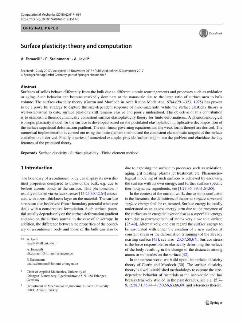
Fig. 1 The bulk domain B0, the surface S0, and the unit normals to thesurface N , all defined in the material configuration. The bulk, surfacedeformation maps, denoted as ϕ, ϕ, respectively, map the material con-figuration to the spatial configuration at time t . The bulk domain Bt , thesurface St and the unit normal to the surface n, all defined in the spatialconfiguration. The bulk and (rank-deficient) surface total deformationgradients are F and F, respectively. Micromechanically the material isdistorted by Fp and Fp into the fictitious intermediate configuration by

dislocation motion. The multiplicative decomposition takes the formF = Fe · Fp and F = Fe · Fp in the bulk and independently on thesurface. The elastic and plastic surface distortions, Fe and Fp, respec-tively, do not necessarily depend on the corresponding bulk distortionsin a similar way as the total surface deformation gradient F dependson the total bulk deformation gradient F, i.e. F = F · I . The elasticcontributions to the total deformations rotate and distort the bulk andthe surface. Both Fp and Fe are in general rank-deficient

Note that from a geometric point of view the surface rightCauchy–Green tensor C and and its plastic counterpart C p arethe pull-backs of i and b−1

e where i is the surface Euclideanmetric in the current configuration and b−1

e is the inverse ofthe surface elastic left Cauchy–Green tensor be. The determi-nants of the elastic and plastic surface distortions are definedby Je := ˆdet Fe > 0 and Jp := ˆdet Fp > 0, so that J = Jp Je.Next, the spatial surface gradient of the spatial surface veloc-ity v(x, t) reads

gradv(x, t) = l = ˙F · F−1. (6)

Noting the elastic-plastic decomposition of the surface defor-mation gradient, Eq. (6) is written as

l = l e + Fe · Lp · F−1e where l e = ˙Fe · F−1

e and

Lp = ˙Fp · F−1p . (7)

with l e and Lp being elastic and plastic surface “velocity gra-dients”. Although the surface velocity gradient l itself andthe elastic contribution l e are spatial quantities, the surfaceplastic velocity gradient Lp is associated with the intermedi-ate configuration which is why in Eq. (7)1 a push-forward tothe current configuration is applied. Finally the surface Liederivative2 of Eq. (5)2 reads

2 The Lie derivative of a spatial surface tensor field f (x, t), relative to

a vector field v is obtained by £v f = ϕ∗(

DDt ϕ

−1∗ ( f ))

, where ϕ−1∗ is

the surface pull-back and ϕ∗ the surface push-forward operators.

123


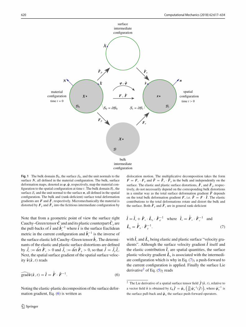
Table 1 Localized force andmoment balances in the bulkand on the surface in thematerial configuration

Force balance DivP + Bp = 0 in B0

Div P + Bp − P · N = 0 on S0

Moment balancea P · Ft = F · P t in B0

P · Ft = F · P t on S0

Bp Force vector per unit volume Bp Surface traction per unit area

The notation {•}p is to denote prescribed quantitiesaBalance of angular momentum results in the symmetry of the bulk and surface Cauchy stress

£v be = ˙be − l · be − be · l t with £v be = F · ˙C−1p · Ft.

(8)

3 Governing equations

The local balance equations of forces and moments in thebulk and on the surface are listed in Table 1.

Restricting the material response to isotropy both on thesurface and in the bulk, the arguments3 of the correspondingfree energies are chosen as

� ≡ �(be,α) and � ≡ �(be, α), (9)

where α and α are the internal variables characterizing thestate of bulk and surface strain hardening, respectively. Nextthe reduced dissipation inequality on the surface is exploited.By differentiating Eq. (9)2 with respect to time, using Eq. (7),and the isotropy assumption, renders

˙�(be, α) = ∂�

∂ be

: ˙be + ∂�

∂α◦ ˙α

=[

∂�

∂ be

· be

]

: [2l + £v be · b−1e ]

+ ∂�

∂α◦ ˙α, (10)

where ◦ is a general contraction operator whose order ofcontraction depends on weather α is scalar or tensorial. Par-ticularizing next the surface Clausius–Plank inequality and

3 Note that the most general set of arguments for the surface freeenergy contains Fp and F in Euclidean space. Imposing the invarianceunder superposed rigid bodymotion onto the intermediate configurationresults in Ce, where Ce is the elastic right Cauchy–Green strain in theintermediate configuration. Imposing further invariance under super-posed rigid body motion on the spatial configuration finally results inbe, see [59] for further details.

using the relation d = lsym4 one expresses the surface dissi-

pation inequality D as

D = τ : d − ˙� ≥ 0 �⇒ D =

[

τ − 2∂�

∂ be

· be

]

: d

+[

2∂�

∂ be

· be

]

:[

−1

2£v be · b−1

e

]

− ∂�

∂α◦ ˙α ≥ 0,

(11)

where the surface Kirchhoff stress τ is the push-forward ofthe surface Piola–Kirchhoff stress S. Thereby the followingrelations hold

τ = F · S · Ft and S = F−1 · P and τ = P · Ft .

(12)

Following the Coleman–Noll exploitation we eventually findthat

τ = 2∂�

∂ be

· be and

Dred = τ :[

−1

2£v be · b−1

e

]

− ∂�

∂α◦ ˙α ≥ 0, (13)

where Eq. (13)1 is the surface constitutive relation and Dred

is the reduced dissipation inequality on the surface.

3.1 Yield condition, maximum dissipation andevolution equations

We now consider a surface yield function defined in the sur-face stress space. Let φ(τ , β) be a general surface yieldfunction dependent on the surface Kirchhoff stress and thestress-like surface internal variables (or conjugate thermody-namical forces to α) denoted by β = ∂�/∂α. Let now E ,∂E and E be defined as

4 The spatial symmetry operator is {•}sym = isym : {•}, where isym =12 [i ⊗ i + i ⊗ i], for spatial second-order surface tensors. Its Material

counterpart is defined as {•}Sym = ISym : {•}, where I

Sym = 12 [ I ⊗ I+

I ⊗ I].

123


E = {τ | φ(τ , β) < 0}, ∂E = {τ | φ(τ , β) = 0} and

E = {τ | φ(τ , β) ≤ 0}, (14)

which are respectively the surface elastic domain, the surfaceyield surface (the boundary of E ) and the surface admissibledomain. Having defined the reduced dissipation inequalityand the yield function on the surface, we state the princi-ple of maximum plastic surface dissipation, which is usedin associative plasticity to derive the flow rule and load-ing/unloading conditions in Kuhn–Tucker form. Locally, for

a prescribed be and prescribed rates˙Cp and ˙α (so that £v be is

fixed), among all possible surface stresses τ ∗ and stress-likeinternal variables β∗ satisfying Eq. (14)3, the plastic dissi-pation Eq. (13)2 is maximized for the actual state (τ

∗, β

∗),

i.e.

Max(

Dred(τ∗, β∗, £v be, ˙α)

)

subject to the constraint

φ(τ ∗, β∗) ≤ 0. (15)

Equivalently, Eq. (15)1 can be written as

[τ − τ ∗] :[

−1

2[£v be] · b−1

e

]

− [β − β∗] ◦ ˙α ≥ 0. (16)

Now the flow rule and loading/unloading conditions canbe obtained as follows: first we transform the inequalityEq. (13)2 into a minimization problem. Next the constrainedminimization problem is reformulated into an unconstrainedproblem by introducing the Lagrangemultiplier γ ≥ 0. Thusthe Lagrangian functional L reads

L := −Dred(τ∗, β∗, £v be, ˙α) + γ φ(τ ∗, β∗). (17)

For the stationary points of L, the derivatives ∂L/∂ τ , ∂L/∂β

and ∂L/∂γ must vanish, thus

− 1

2£v be = γ

∂φ

∂ τ· be, ˙α = γ

∂φ

∂β

γ ≥ 0, φ(τ , β) ≤ 0, γ φ(τ , β) = 0. (18)

Remark 3 For isotropy the flow rule Eq. (18)1 is equivalentto

γ ∂φ/∂ τ = Fe · Lp · F−1e , (19)

which may be shown as follows5: by multiplying both sidesof the above relation by be, noting Fe · Lp · F−1

e = l − l e andthat the left hand side in Eq. (19) is symmetric (due to the

5 Note that in Eq. (19) it is assumed that plastic spin W p = 0, thus Lp

is symmetric.

isotropy assumption the tensor be and ∂φ/∂ τ commute), weobtain

γ∂φ

∂ τ· be = 1

2[l · be + be · l t − ˙be] with

˙be = ˙Fe · Fte + Ft

e · ˙Fe, (20)

which proves the equivalence (see also Eq. (8)1). The flowrule in Eq. (19) can also be reformulated for the intermediateconfiguration resulting in Lp = γ N

φ· C e, where N

φ=

F−1e · [∂φ/∂ τ ] · F−t

e is the normal to the surface yield surfacein the intermediate configuration. The spatial counterpart ofthe normal N

φis denoted by n

φ= ∂φ/∂ τ . Furthermore,

a pressure-independent surface yield condition implies anisochoric plastic deformation, i.e Jp = 1, as follows: firstfrom J = Je Jp we have

ln J = ln( Je Jp) �⇒ D ln J

Dt

= D ln JeDt

+ D ln JpDt

�⇒˙JJ

=˙JeJe

+˙JpJp

. (21)

Next expanding the time derivative of ˙Je results in6

˙Je = Je trace(d − γ nφ) with ˙J

= J trace(d) �⇒ D ln JpDt

= γ tracenφ. (22)

Therefore if tracenφ

= 0, then Jp = 1.

3.2 VonMises-type surface yield criterion and thecase of decoupled surface volumetric–deviatoricresponse

In this section we consider the von Mises-type surface yieldcondition7 as a function of the surface Kirchhoff stress tensoras

φ(τ , Fp) := ‖dev(τ )‖ −√

2

3[σY + K (Fp)] ≤ 0, (23)

where σY denotes the surface yield stress, K is a (non)linearfunction of Fp, the surface hardening variable, which deter-

6 The surface trace operator for spatial second order tensor is definedas trace{•} = {•} : i . In the material configuration the surface traceoperator is defined correspondingly as Trace{•} = {•} : I .7 Note that henceforth only the classical example for metal plasticity,i.e. the vonMises-type yield criterion is considered. Thus, we only takeinto account the simplest plasticity model, i.e. J2 type flow theory withisotropic hardening to be developed on the surface. This is to motivatea surface elastoplasticity model and examine its computational aspects.

123


mines the isotropic hardening behavior of the surface anddev{•} = {•} − 1

2 trace{•}i is the spatial surface deviatoricoperator. The factor

√2/3 is used for the sake of analogy

with classical bulk von Mises yield criterion.Next we introduce briefly the kinematics of the surface

deviatoric–volumetric multiplicative split according to thechosen yield criterion Eq. (23). Let F iso and Fvol denote thevolume-preserving (angle-changing) and volumetric part ofthe surface deformation gradient8, hence F = Fvol · F iso

where det F iso = J iso = 1. Consequently F iso, Fvol, C iso andbiso are defined as

F iso := J−1/2 F, Fvol := J 1/2 I,

C iso := [F iso]t · F iso ≡ J−1C and

biso := F iso · [F iso]t ≡ J−1 b. (24)

Note that the same volumetric–isochoric decoupling can beapplied on the plastic and elastic contribution of any of theabove strain measures. We also point out that the exponents−1/2, 1/2 and −1 appearing in Eq. (24) are due to thelower-dimensional nature of the surface. The correspondingexponents in the bulk assume the familiar values −1/3, 1/3and −2/3.

3.3 Model problem: decoupled hyperelastic stressresponse

As a model problem, and as the basis for the numericalexamples9, we consider the following decoupled surface freeenergy

� = � iso(bisoe ) + �vol( Je) with

� iso = 1

2μ

[

tracebisoe − 2

]

and

�vol = 1

2κ

[

1

2[ J 2e − 1] − ln Je

]

, (25)

where � iso(be) and �vol( Je) are the isochoric and volumetriccontribution to the total surface free energy and biso

e = J−1e be.

The surface shear modulus and surface bulk modulus aredenoted respectively by μ and κ . Next, to obtain the surface

8 The term volumetric has a different meaning on the surface. A surfacevolumetric deformation describes a deformation that changes the area.A volumetric deformation in the bulk however changes the volume.Nonetheless, we use the same term for both the bulk and the surface forthe sake of simplicity.9 Wemention the assumptionsmade for the numerical part of the currentmanuscript: first, the surface stress response is isotropic. Second, theplastic spin on the surface is assumed to vanish. Third, the main focushere is on metal plasticity meaning that plastic yielding is isochoric, i.e.Jp = 1, which justifies the decoupling of the surface strain energy. Notethat the same assumptions are also made for the bulk elastoplasticity.

Kirchhoff stress τ from the energy given above we first notethat

tracebisoe = TraceC iso

e or tracebisoe = C iso : [C iso

p ]−1 with

C isoe = J−1

e C e, Je = [DetC e]1/2. (26)

Subsequently usingEq. (26) one can re-parameterizeEq. (25)in material quantities. Consequently the surface Kirchhoffstress reads

τ = 2Fe · ∂�

∂ C e

· Fte = 2F · ∂�(C, C p)

∂ C· Ft

= 1

2κ[ J 2e − 1]i

︸︷︷︸

τ vol

+ μdevbisoe

︸︷︷︸

τ iso

, (27)

where the intermediate steps to derive Eq. (27) are given as

τ vol = 1

2κ Fe ·

[

[ J2e − 1]C−1e

]

· Fte and

τ iso = μ J−1e F ·

[

−1

2C−1

[

C : (C isop )−1

]

+ (C isop )−1 : I

Sym

]

· Ft

= μ J−1e F ·

[

Dev(C isop )−1

]

· Ft, (28)

with Dev{•} := {•} − 12 [C : {•}]C−1 being the material

surface deviatoric operator and ISym = ∂ C/∂ C. Note that in

the derivation above it is implied that J = Je since J = Je Jpand Jp = 1. Consequently C iso

p = C p. Next the isochoric andvolumetric surface elasticity tensors of the model problemEq. (25) both in the material and spatial configurations aregiven as

Cvole = 2

∂ Svol

∂ C e

= κ

[

detC eC−1e ⊗ C−1

e + ∂ C−1e

∂ C e

[

detC e − 1]

]

with [cvole ]i jkl = [Fe]i I [Fe] j J [Fe]kK [Fe]l L [Cvol

e ]I J K L

�⇒ cvole = κ

[

J2e i ⊗ i + isym[ J2e − 1]]

, (29)

and

Cisoe = ∂ Siso

∂ C= 2μ

[

(C isop )−1 − 1

2

[

(C isop )−1 : C

]

C−1]

⊗[

−1

2J−1

e C−1]

+ 2μ J−1e C−1 ⊗

[

−1

2(C iso

p )−1 : ISym

]

− μ J−1e C : (C iso

p )−1[

−1

2

[

C−1⊗C−1 + C−1⊗C−1]

]

with [cisoe ]i jkl = [F]i I [F] j J [F]kK [F]l L [Ciso

e ]I J K L �⇒ cisoe

= μtracebisoe [isym − 1

2i ⊗ i] − μ[devbiso

e ⊗ i + i ⊗ devbisoe ],(30)

123


where

Svol = 1

2κ

[

[ J2e − 1]C−1e

]

and Siso = μ J−1e

[

Dev(C isop )−1

]

.

(31)

The volumetric surface elasticity tensors in the material andspatial configuration in the above are denoted by C

vole and cvol

e ,respectively. Their isochoric counterparts are denoted by C

isoe

and cisoe , respectively.

Now Considering the definition of τ iso in Eq. (27) andn

φ= devτ/‖devτ‖, one can simplify the flow rule Eq. (18)

as follows10

−1

2£v be = γ n

φ· be = γ Jenφ

·[

1

2tracebiso

e i + devbisoe

]

= γ Je

[

1

2tracebiso

e nφ

+ nφ

· μdevbisoe

μ‖devbisoe ‖

μ‖devbisoe ‖

μ

]

= γ Je

[

1

2tracebiso

e nφ

+ n2φ�

��‖devτ‖

μ

]

≈ 1

2γ Jetracebiso

e nφ, (32)

with ‖devτ‖/μ ∼= 10−3 for metals and thus neglected. UsingEq. (8)2 the simplified surface flow rule (the last term inEq. (32)) can also be given in the material configuration as

˙C−1p = −γ tracebe F−1 · n

φ· F−t. (33)

Finally to complete the surface plasticity formulation, theevolution of the hardening variable Fp in terms of the plasticmultiplier (Lagrange multiplier or consistency parameter) γ ,and the consistency condition are now given as follows

˙Fp =√

2

3γ and γ

˙φ(τ , Fp) = 0. (34)

3.3.1 Return mapping algorithm

In this section the time discretization of the model intro-duced in the previous section, i.e. the integration algorithmfor J2 type plasticity on the surface together with the returnmapping algorithm are given. Due to the path-dependence ofthe surface plasticity model, the surface stress tensor is thesolution of a constitutive initial value problem meaning thatthe surface stress tensor is not only a function of the instan-taneous value of the surface strain but also depends on thehistory of surface strain. Therefore an appropriate numericalalgorithm for integration of the rate constitutive equations isa requirement in the finite element simulation of such mod-els. In doing so, we assume the data {ϕτ , [be]τ , [Fp]τ , Fτ } is10 Alternatively, a formulation adapting the flow rule in [62] to surfaceplasticity is possible.

known at time tτ . Consequently the surface Kirchhoff stresstensor τ τ is also known through Eq. (27). We start by pro-viding the discretized evolution Eqs. (33) and (34)1 in thematerial configuration as

[C−1p ]τ+1 − [C−1

p ]τ = −γ[

[C−1p ]τ+1 : [C−1]τ+1

]

F−1τ+1

· [nφ]τ+1 · F−t

τ+1 and

[Fp]τ+1 − [Fp]τ =√

2

3γ, (35)

where τ denotes the time step and time discretization schemeis backward-Euler. The spatial counterpart of the above readsnow

[bisoe ]τ+1 = F iso

τ+1 · [bisoe ]τ · (F iso

τ+1)t

− γ tracebisoτ+1[nφ

]τ+1 with

F isoτ+1 = F iso

τ+1 · (F isoτ )−1. (36)

Next we define a trial elastic state, based on the known dataas follows:

[C−1p ]trialτ+1 = [C−1

p ]τ , [Fp]trialτ+1 = [Fp]τ ,[biso

e ]trialτ+1 = F isoτ+1 · [biso

e ]τ · [F isoτ+1]t and

τ trialτ+1 = 1

2κ

[

[ J 2e ]τ+1 − 1]

i + μdev[bisoe ]trialτ+1. (37)

Having obtained the trial state, one can define a temporally-discretized trial surface yield condition φ trial, using Eq. (23)as

φ trialτ+1 = φ(τ trial

τ+1, [Fp]τ ) := ‖devτ trialτ+1‖

−√

2

3[σY + K ([Fp]τ )], (38)

from which the following two alternatives arise:

if φ trialτ+1 ≤ 0 trial step is elastic ⇒ γ

= 0 and {•}τ+1 = {•}trialτ+1

if φ trialτ+1 > 0 trial step is plastic ⇒ γ

> 0 and {•}τ+1 �={•}trialτ+1 and return mapping.

(39)

In case the second situation above arises, since γ > 0, tofind γ , we require φ(τ τ+1, [Fp]τ+1) = 0. Thus we have

φ(τ τ+1, [Fp]τ+1) = ‖devτ τ+1‖ −√

2

3[σY + K ([Fp]τ+1)]

= ‖devτ trialτ+1‖ − μγ trace(biso

e )trialτ+1

−√

2

3[σY + K ([Fp]τ+1)] = 0. (40)

123


In general φ(τ τ+1, [Fp]τ+1) is a non-linear11 function ofγ ,and thus to solve Eq. (40), one requires the use of Newton–Raphson method.

Remark 4 In deriving the last term in Eq. (40) we made useof the following relation

‖devτ τ+1‖ + μγ trace(bisoe )trialτ+1 = ‖devτ trial

τ+1‖. (41)

To prove the above we recall the definition of τ iso in Eq. (27),the flow rule Eq. (36)1, Eq. (37)4, tracebiso

e = trace(bisoe )trial

and nφ

= devτ/‖devτ‖. We then write

devτ τ+1 = μdev(bisoe )τ+1 = μdev(bisoe )trialτ+1

− μγ trace(bisoe )trialτ+1[nφ]τ+1

�⇒[

‖devτ τ+1‖ + μγ trace(bisoe )trialτ+1

]

[nφ]τ+1

= ‖devτ trialτ+1‖[nφ

]trialτ+1. (42)

From the last term above it is implied that

‖devτ τ+1‖ + μγ trace(bisoe )trialτ+1 = ‖devτ trial

τ+1‖ and

[nφ]τ+1 = [n

φ]trialτ+1, (43)

where Eq. (43)1 concludes the proof.

Having found γ , we finally provide the update formula for[biso

e ]τ+1 and τ τ+1 as follows

[bisoe ]τ+1 = [biso

e ]trialτ+1 − γ trace(bisoe )trialτ+1[nφ

]τ+1 and

τ τ+1 = τ volτ+1 + μdev(biso

e )trialτ+1 − γ μtrace(bisoe )trialτ+1[nφ

]τ+1.

(44)

3.3.2 Algorithmic elastoplastic tangent modulus

The objective of this section is to exactly linearize the updateformula provided for the surfaceKirchhoff stress in Eq. (44)2in order to obtain quadratic convergence associated with theNewton–Raphson method. The linearization of the first twoterms in Eq. (44)2 are given by Eqs. 29 and (30), respec-tively. To linearize the last term in Eq. (44)2 we make use ofEq. (40)3 and the following12

devτ = F · DevS · Ft, τ = F · S · Ft,

trace(bisoe )trialτ+1 = J−1C : (C iso)−1

p and (45)

‖devτ‖ =√

Fi I [DevS]I J Fj J Fi K [DevS]KM FjM

=√

[DevS]I J [DevS]KMCI K CJM . (46)

11 This is the case when K ([Fp]τ+1) is a non-linear function of [Fp]τ+1

and consequently a non-linear function of γ since [Fp]τ+1 = [Fp]τ +√2/3γ .

12 In the following derivations we drop the super- and sub-index trial andτ + 1 for the sake of brevity.

Using the chain rule and Eq. (46)2, the linearization of‖devτ‖ now reads

2∂‖devτ‖∂CAB

= [Cisoe ]I J AB[N

φ]KMCI K CJM

+ 2‖DevS‖[Nφ]AI [Nφ

]BJ CI J‖devτ‖Lin

= 2F · ∂‖devτ‖∂ C

· Ft

= μtracebisoe nφ

+ 2dev(nφ

· devbisoe )

= μtracebisoe nφ

+ 2‖devτ‖dev(nφ

· nφ). (47)

Thus, the linearization of nφbecomes

[nφ]Lin = ciso

e /‖devτ‖ − 1

‖devτ‖ nφ

⊗[

μtracebisoe nφ


· nφ)]

. (48)

Next the linearization of Eq. (46)3 reads

[tracebisoe ]Lin = 2F · ∂( J−1C−1

p : C)

∂ C· Ft = 2devbiso

e . (49)

What remains now is to linearizeγ . By using Eq. (40)3 andthe results above we have

‖devτ‖Lin − μ[

[γ ]Lintracebisoe + γ [tracebisoe ]Lin]

− 2

3[γ ]Lin dK (Fp)

d Fp

= 0 �⇒ [γ ]Lin = ‖devτ‖Lin − μγ [tracebisoe ]Linμtracebisoe + 2

3

dK (Fp)

d Fp

�⇒ [γ ]Lin

=[

μtracebisoe nφ


· nφ)]

− 2μγ devbisoe

μtracebisoe + 2

3

dK (Fp)

d Fp

. (50)

Note that in the derivations above ‖devτ‖Lin, [γ ]Lin and[tracebiso

e ]Lin are vectors and [nφ]Lin is a fourth-order tensor.

Having found the linearization of the terms appearing in theupdate formula of the stress Eq. (44)2, the surface algorithmicelastoplastic tangent modulus calg

ep is now given as

calgep = cvole + cisoe − γ μtracebisoe[

cisoe /‖devτ‖ − 1

‖devτ‖ nφ⊗

[

μtracebisoe nφ


· nφ)]

]

− 2γ μnφ

⊗ devbisoe − μtracebisoe[

μtracebisoe nφ

⊗ nφ

+ 2‖devτ‖ sym(

nφ

⊗ dev(nφ

· nφ))]

− 2μγ nφ

⊗ devbisoe

μtracebisoe + 2

3

dK (Fp)

dFp

,

(51)

where sym(•) is the major symmetrization operator.

123


4 Computational framework

In this section we establish a numerical framework thatencompasses elastoplasticity of surfaces. For further detailsof the finite element implementation on surfaces see [18–22] . The weak form, together with its temporal and spatialdiscretizations will be presented next. The localized forcebalance equations in the bulk and on the surface given inTable 1 are tested with vector valued test functions δϕ ∈H 1(B0) and δϕ ∈ H 1(S0), respectively. By integrating theresult over all domains in the material configuration, usingthe bulk and surface divergence theorems and the superficial-ity properties of the surface Piola stress, the weak form ofthe balance of linear momentum reads

∫

B0

P : GradδϕdV +∫

S0

P : GradδϕdA

−∫

B0

δϕ · BpdV −∫

S0

δϕ · BpdA = 0,

∀δϕ ∈ H 1(B0), ∀δϕ ∈ H 1(S0).

(52)

Since the surface stress derived in the previous section isthe surface Kirchhoff stress, in the weak form formulation,relation Eq. (12)3 is used to convert τ to P .

In what follows, a classical Euler-backward integrationscheme is employed. Next, the spatial discretization of theproblem domain is performed using the Bubnov-Galerkinfinite element method. In order to have a straightforwardand efficient implementation of the finite element method,the surface elements are chosen to be consistent with thebulk elements. For example, if the bulk is discretized usingtriquadratic elements, then biquadratic surface elements areused. This choice has the advantage that facets to which onlyone bulk element is attached can be regarded as a surfaceelement.

The domains B0 and S0 are discretized into a set of bulkand surface elements

Bh0 ≈

nBel⋃

β=1

Bβ0 and Sh

0 ≈nSel⋃

γ=1

Sγ0 , (53)

where nBel and nSel denote the number of bulk and surfaceelements, respectively. The geometry of the bulk and surfaceare approximated as a function of the natural coordinatesξ ∈ [−1, 1]3 and ξ ∈ [−1, 1]2 assigned to the bulk and thesurface, respectively, using standard interpolations accordingto the isoparametric concept as follows:

X |Bβ0

≈ Xh (ξ) =nnB∑

i=1

Ni (ξ) X i ,

X |Sγ0

≈ Xh(

ξ)

=nnS∑

i=1

N i(

ξ)

X i ,

ϕ |Bβ0

≈ ϕh (ξ) =nnB∑

i=1

Ni (ξ) ϕi ,

ϕ |Sγ0

≈ ϕh(

ξ)

=nnS∑

i=1

N i(

ξ)

ϕi , (54)

where the shape functions of the bulk and surface elementsat a local node i are denoted as Ni and N i , respectively.The bulk and surface elements consist of nnB and nnS nodesrespectively. The numerical integration in the bulk and on thesurface is performed using Gaussian quadrature formula, see[19] for further details.

Remark 5 The surface is a two-dimensional manifold in thethree-dimensional space and therefore can be described bytwo surface coordinates. The corresponding tangent vectorsto the coordinate lines i.e. the covariant surface basis vectorsare obtained by taking the derivative of the position vectoron the surface with respect to the coordinates. The covariantbasis vectors furnish the normal to the surface via a vectorproduct. The surface normal is then normalized by its mag-nitude to obtain the unit normal to the surface, see [36,64].

Now the fully discrete (spatially and temporally) formof mechanical residual associated with the global node I isdefined by

[

totR I]

τ+1=

∫

B0

Pτ+1 · GradN IdV −∫

B0

N I Bpτ+1dV

+∫

S0

Pτ+1 · Grad N IdA −∫

S0

N I Bpτ+1dA.

(55)

To solve Eq. (55), a Newton–Raphson scheme is utilized,which results in the introduction of algorithmic stiffnessmatrix in the bulk and on the surface, respectively, as fol-lows:

KIJ = ∂R I

∂ϕ J=

∫

B0

Grad N I · Aτ+1 · Grad N JdV and,

KIJ = ∂R I

∂ϕ J=

∫

S0

Grad N I · Aτ+1 · Grad N JdA,

(56)

where A = ∂F P and A = ∂F P . The spatial surface elasto-plastic tangent modulus calg

ep derived in the previous section

can be connected to A, in index notation, using the relation

AaBcD = F−1Bb

[[calgep ]abcd + τacδbd

]

F−1Dd . (57)

123


Table 2 Material propertiesassumed in the numericalexamples

Bulk Surface

Lamé constant μ 80193.8 N/mm2 μ 80193.8 N/mm

Lamé constant λ 110743 N/mm2 λ 110743 N/mm

Compression modulus κ 164206.0 N/mm2 κ 190936.8 N/mm

Hardening coefficient Kh − 12.924 N/mm2 Kh − 12.924 N/mm

Yield stress σY 0 N/mm2 σY 0 N/mm

Initial flow stress σ0 450 N/mm2 σ0 450 N/mm

Residual flow stress σ∞ 715 N/mm2 σ∞ 715 N/mm

Saturation exponent δ 16.93 δ 16.93

Note that κ = λ + 2/3μ and κ = λ + μ

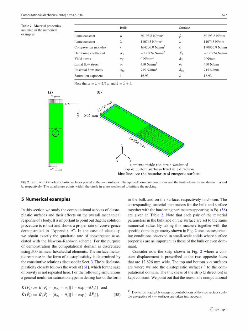
Fig. 2 Strip with two elastoplastic surfaces placed at the x–y surfaces. The applied boundary conditions and the finite elements are shown in a andb, respectively. The quadrature points within the circle in a are weakened to initiate the necking

5 Numerical examples

In this section we study the computational aspects of elasto-plastic surfaces and their effects on the overall mechanicalresponse of a body. It is important to point out that the solutionprocedure is robust and shows a proper rate of convergencedemonstrated in “Appendix A”. In the case of elasticity,we obtain exactly the quadratic rate of convergence asso-ciated with the Newton–Raphson scheme. For the purposeof demonstration the computational domain is discretizedusing 500 trilinear hexahedral elements. The surface inelas-tic response in the form of elastoplasticity is determined bythe constitutive relations discussed inSect. 3. Thebulk elasto-plasticity closely follows the work of [61], which for the sakeof brevity is not repeated here. For the following simulationsa general nonlinear saturation type hardening law of the form

K (Fp) := KhFp + [σ∞ − σ0][1 − exp(−δFp)] and

K (Fp) := Kh Fp + [σ∞ − σ0][1 − exp(−δ Fp)], (58)

in the bulk and on the surface, respectively is chosen. Thecorresponding material parameters for the bulk and surfacetogether with the hardening parameters appearing in Eq. (58)are given in Table 2. Note that each pair of the materialparameters in the bulk and on the surface are set to the samenumerical value. By taking this measure together with thespecific domain geometry shown in Fig. 2 one assures creat-ing conditions observed in small-scale solids where surfaceproperties are as important as those of the bulk or even dom-inant.

Consider now the strip shown in Fig. 2 where a con-stant displacement is prescribed at the two opposite facesthat are 12.826 mm wide. The top and bottom x-y surfacesare where we add the elastoplastic surfaces13 to the com-putational domain. The thickness of the strip (z direction) iskept constant. We point out that the reason the computational

13 Due to the negligible energetic contributions of the side surfaces onlythe energetics of x-y surfaces are taken into account.

123


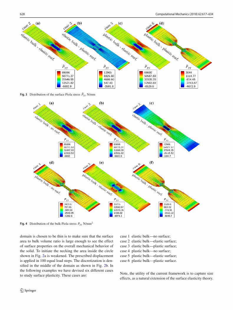
Fig. 3 Distribution of the surface Piola stress Pyy N/mm

Fig. 4 Distribution of the bulk Piola stress Pyy N/mm2

domain is chosen to be thin is to make sure that the surfacearea to bulk volume ratio is large enough to see the effectof surface properties on the overall mechanical behavior ofthe solid. To initiate the necking the area inside the circleshown in Fig. 2a is weakened. The prescribed displacementis applied in 100 equal load steps. The discretization is den-sified in the middle of the domain as shown in Fig. 2b. Inthe following examples we have devised six different casesto study surface plasticity. These cases are:

case 1 elastic bulk—no surface;case 2 elastic bulk—elastic surface;case 3 elastic bulk—plastic surface;case 4 plastic bulk—no surface;case 5 plastic bulk—elastic surface;case 6 plastic bulk—plastic surface.

Note, the utility of the current framework is to capture sizeeffects, as a natural extension of the surface elasticity theory.

123


Fig. 5 Distribution of the norm of the elastic deviatoric Cauchy–Green tensor ‖bisoe ‖ in the bulk (a)–(c) and ‖bisoe ‖ on the surface (d), (e)

Fig. 6 Distribution of the hardening variable Fp in the bulk (a)–(c) and Fp on the surface (d), (e)

123


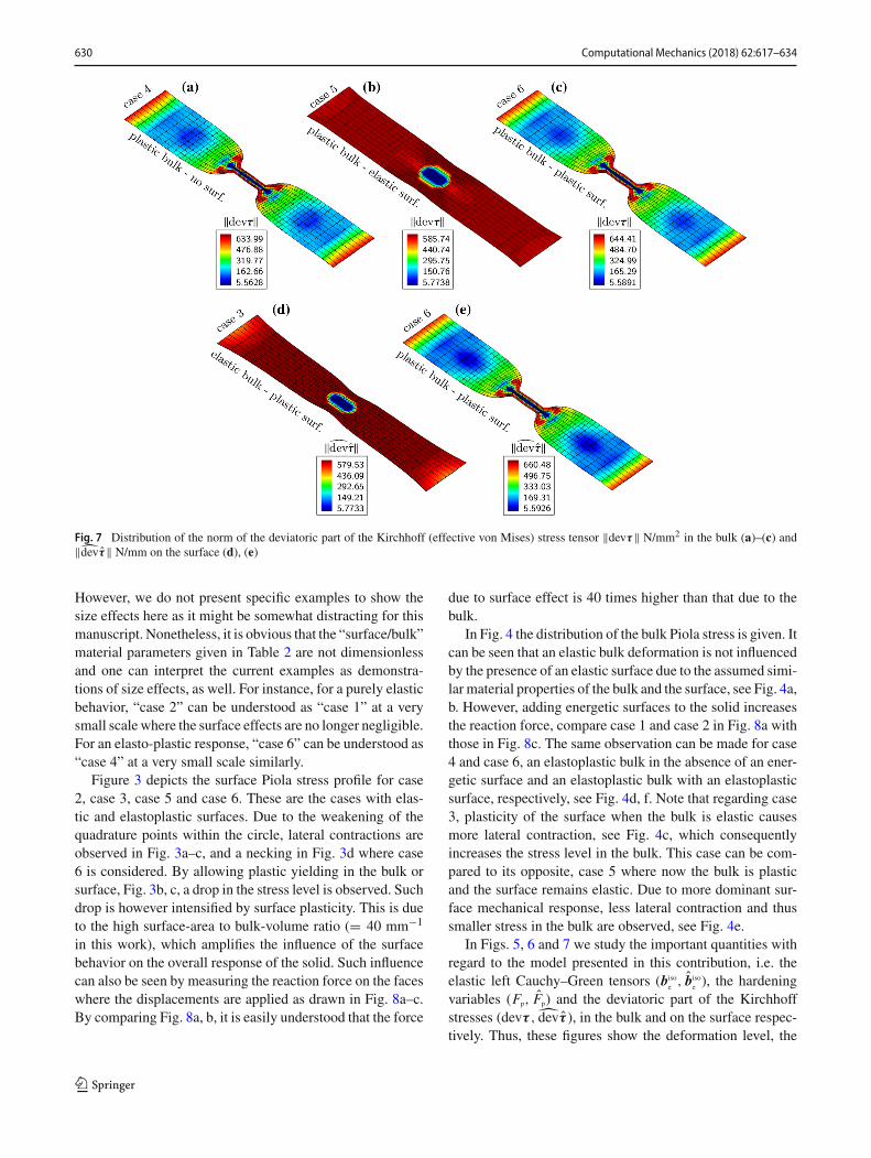
Fig. 7 Distribution of the norm of the deviatoric part of the Kirchhoff (effective von Mises) stress tensor ‖devτ‖ N/mm2 in the bulk (a)–(c) and‖devτ‖ N/mm on the surface (d), (e)

However, we do not present specific examples to show thesize effects here as it might be somewhat distracting for thismanuscript. Nonetheless, it is obvious that the “surface/bulk”material parameters given in Table 2 are not dimensionlessand one can interpret the current examples as demonstra-tions of size effects, as well. For instance, for a purely elasticbehavior, “case 2” can be understood as “case 1” at a verysmall scale where the surface effects are no longer negligible.For an elasto-plastic response, “case 6” can be understood as“case 4” at a very small scale similarly.

Figure 3 depicts the surface Piola stress profile for case2, case 3, case 5 and case 6. These are the cases with elas-tic and elastoplastic surfaces. Due to the weakening of thequadrature points within the circle, lateral contractions areobserved in Fig. 3a–c, and a necking in Fig. 3d where case6 is considered. By allowing plastic yielding in the bulk orsurface, Fig. 3b, c, a drop in the stress level is observed. Suchdrop is however intensified by surface plasticity. This is dueto the high surface-area to bulk-volume ratio (= 40 mm−1

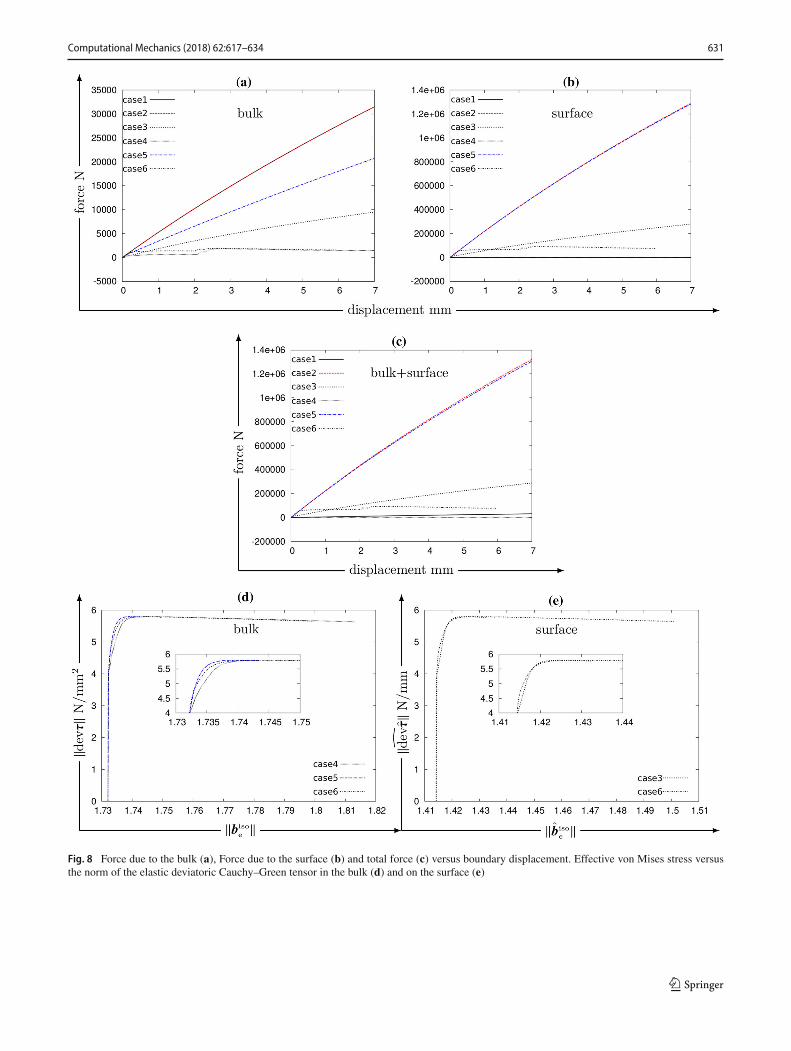
in this work), which amplifies the influence of the surfacebehavior on the overall response of the solid. Such influencecan also be seen by measuring the reaction force on the faceswhere the displacements are applied as drawn in Fig. 8a–c.By comparing Fig. 8a, b, it is easily understood that the force

due to surface effect is 40 times higher than that due to thebulk.

In Fig. 4 the distribution of the bulk Piola stress is given. Itcan be seen that an elastic bulk deformation is not influencedby the presence of an elastic surface due to the assumed simi-lar material properties of the bulk and the surface, see Fig. 4a,b. However, adding energetic surfaces to the solid increasesthe reaction force, compare case 1 and case 2 in Fig. 8a withthose in Fig. 8c. The same observation can be made for case4 and case 6, an elastoplastic bulk in the absence of an ener-getic surface and an elastoplastic bulk with an elastoplasticsurface, respectively, see Fig. 4d, f. Note that regarding case3, plasticity of the surface when the bulk is elastic causesmore lateral contraction, see Fig. 4c, which consequentlyincreases the stress level in the bulk. This case can be com-pared to its opposite, case 5 where now the bulk is plasticand the surface remains elastic. Due to more dominant sur-face mechanical response, less lateral contraction and thussmaller stress in the bulk are observed, see Fig. 4e.

In Figs. 5, 6 and 7 we study the important quantities withregard to the model presented in this contribution, i.e. theelastic left Cauchy–Green tensors (biso

e , bisoe ), the hardening

variables (Fp, Fp) and the deviatoric part of the Kirchhoffstresses (devτ , devτ ), in the bulk and on the surface respec-tively. Thus, these figures show the deformation level, the

123


Fig. 8 Force due to the bulk (a), Force due to the surface (b) and total force (c) versus boundary displacement. Effective von Mises stress versusthe norm of the elastic deviatoric Cauchy–Green tensor in the bulk (d) and on the surface (e)

123


plastic yielding and von Mises effective stress of the herepresented examples, respectively, for all the relevant cases,i.e case 3–case 6. In the first row of Fig. 5 the bulk is alwayselastoplastic while the surface ranges from being not presentto being elastoplastic. It is clear that with an elastic surface,the elastic deviatoric deformation is constrained, see Fig. 5b.Another interesting observation is that even when the surfaceis allowed to be elastoplastic still a lower level of deforma-tion is achieved as shown in Fig. 5c compared to Fig. 5a.These dissimilar levels of deformations consequently lead todifferent evolutions of the equivalent plastic distortion, seeFig. 6a–c, and the effective stress in the bulk, see Figs. 7a–cand 8d. FromFig. 8d, which is drawn for one node in themid-dle of the domain, one can also conclude that the strongestplastic yielding in the bulk occurs for case 4 and the low-est for case 5. Figures 5, 6 and 7d, e show the elastoplasticbehavior of the surface.

It is clear thatwhen the bulk remains elastic, surface plasticdeformation is constrained (see Fig. 5d compared to Fig. 5e),thus much lower values of the surface plastic equivalent dis-tortion (see Fig. 6d compared to Fig. 6e) and von Miseseffective stress are obtained (see Fig. 7d compared to Fig. 7e).We also point out that although the evolutions of the effectivevon Mises stresses on the surface for one node in the middleof the surface for case 5 and case 6 are almost the same (seeFig. 8e), their overall behavior is noticeably different whichcan be observed from the measured reaction force due to thesurface, see Fig. 8b.

6 Summary and conclusion

A three-dimensional formulation and finite element frame-work for elastoplastic continua encased by elastoplasticsurfaces is presented. The surfaces are endowed with theirown elastoplastic constitutive behavior whereby the freeenergies capture the hyperelastic part of the constitutiverelations. The correspondingweak formsof the balance equa-tions including the contributions from the surfaces are givenin detail. The balance equations are fully discretized in spaceusing the finite element method. The exact consistent stiff-ness matrices in the bulk and on the surface are incorporated.A three-dimensional numerical example serves to elucidate

the role of surface plasticity on the overall response of abody. For the sake of demonstration, we assumed that thesurface response is isotropic, the plastic spin on the surfaceis zero and the plastic yielding of the surface is isochoric.The geometry of the computational domain is chosen so asto have a large surface area to bulk volume ratio. It is shownif the surface remains elastic, the otherwise-typical neckingin the bulk is prevented and vice versa. However, lateral con-traction is higher when the surface is elastoplastic and thebulk remains elastic which emphasizes the dominant role ofthe surface on the overall mechanical response of the solid.Necking initiates and develops to its complete form whenthe elastoplastic bulk is either not wrapped by an energeticsurface or both the surface and the bulk are allowed to yieldplastically. Although for both of the above cases the neckingis fully developed and is similar in terms of deformation, theiroverall reaction forces are substantially different. It is seenthat for the former case the force monotonically increases,whereas for the latter case the force, after an initial increase,continues to decline. The further extension of this work tonon-coherent interfaces will be elaborated in a future contri-bution in which a traction-separation law similar to that ofthe cohesive zone model is assumed to relate the interfacetraction to the displacement jump across the interface. Inaddition, it is straightforward to employ more sophisticatedplasticity models taking into account for instance anisotropy.Moreover, an investigation of the influences of the bulk andsurface inelasticity on the thermomechanical response of abody is of great importance. Regarding the numerical imple-mentation, one needs to also consider measures to tackle thevolumetric locking and also a mesh densification study tomake sure the sufficient convergence of the results. Theseextensions shall be discussed in later contributions.

Acknowledgements The first author gratefully acknowledges the sup-port by the Cluster of Excellence “Engineering ofAdvancedMaterials”.

Appendix A: Convergence behavior

In this section we present some data on the convergencebehavior of the computational problem at hand. The L2

norms of the residual of few increments for some of the casesdiscussed in Sect. 5 are given in Table 3.

123


Table 3 L2 norm of the residual for case 4, case 3 and case 6

Increment Iteration

Case 4: plastic bulk—no surface

1 1.08e+3 3.99e+0 3.20e+0 1.67e+0 2.24e−02 2.04e−04 7.62e−06 2.74e−08

26 1.07e+03 2.15e−01 2.05e−01 2.02e−02 7.54e−03 2.49e−03 4.71e−04 3.33e−06 2.17e−09

31 1.07e+03 2.75e−01 5.12e−02 6.09e−04 3.12e−06 2.70e−08

100 1.72e+03 4.69e−01 9.28e−02 2.57e−02 7.99e−03 1.87e−03 2.35e−04 3.17e−06 6.87e−09

Case 3: elastic bulk—plastic surface

1 4.44e+04 3.46e+00-2 8.11e−01 3.68e−01 1.48e−03 1.22e−05 8.23e−09

26 4.29e+04 3.79e−02 4.43e−03 6.96e−07 7.55e−10

60 4.12e+04 2.62e−02 2.23e−03 3.24e−05 1.80e−08

100 4.10e+04 2.51e−02 2.286e−03 1.06e−06 3.38e−8 8.36e−10

Case 6: plastic bulk—plastic surface

1 1.63e+04 9.76e−02 3.46e−03 3.01e−06 4.43e−08

26 4.32e+04 1.18e−01 3.00e−02 8.28e−04 5.92e−06 1.45e−08

40 1.61e+04 1.33e−01 1.40e−02 8.66e−04 6.77e−06 1.82e−08 3.94e−10

100 8.06e+04 1.00e+00 1.10e−02 2.41e−04 8.37e−06 1.61e−09

References

1. AdamsonW,GastAP (1997) Physical chemistry of surfaces.Wiley,New York

2. Bellet M (2001) Implementation of surface tension with wall adhe-sion effects in a three-dimensional finite element model for fluidflow. Commun Numer Methods Eng 17(8):563–579

3. Benveniste Y (2013) Models of thin interphases and the effec-tive medium approximation in composite media with curvilinearlyanisotropic coated inclusions. Int J Eng Sci 72:140–154

4. Benveniste Y, Miloh T (2001) Imperfect soft and stiff interfaces intwo-dimensional elasticity. Mech Mater 33(6):309–323

5. Bottomley DJ, Ogino T (2001) Alternative to the Shuttleworth for-mulation of solid surface stress. Phys Rev B 63:165412

6. Cammarata RC (1994) Surface and interface stress effects in thinfilms. Prog Surf Sci 46(1):1–38

7. Cammarata RC (1997) Surface and interface stress effects on inter-facial and nanostructured materials. Mater Sci Eng A 237(2):180–184

8. Chatzigeorgiou G, Javili A, Steinmann P (2013) Multiscale mod-elling for composites with energetic interfaces at the micro- ornanoscale. Math Mech Solids 20:1130–1145

9. DaherN,MauginGA(1986)Themethodof virtual power in contin-uum mechanics application to media presenting singular surfacesand interfaces. Acta Mech 60(3–4):217–240

10. Davydov D, Javili A, Steinmann P (2013) Onmolecular statics andsurface-enhanced continuummodeling of nano-structures. ComputMater Sci 69:510–519

11. de Souza Neto EA, Peric D, Owen DRJ (2011) Computationalmethods for plasticity: theory and applications. Wiley, Chichester

12. dell’Isola F, RomanoA (1987)On the derivation of thermomechan-ical balance equations for continuous systems with a nonmaterialinterface. Int J Eng Sci 25:1459–1468

13. Dingreville R, Qu J, Cherkaoui M (2005) Surface free energy andits effect on the elastic behavior of nano-sized particles, wires andfilms. J Mech Phys Solids 53(8):1827–1854

14. Duan HL, Karihaloo BL (2007) Effective thermal conductivitiesof heterogeneous media containing multiple imperfectly bondedinclusions. Phys Rev B 75(6):064206

15. Duan HL, Wang J, Huang ZP, Karihaloo BL (2005a) Eshelby for-malism for nano-inhomogeneities. Proc R Soc A Math Phys EngSci 461(2062):3335–3353

16. Duan HL, Wang J, Huang ZP, Karihaloo BL (2005b) Size-dependent effective elastic constants of solids containing nano-inhomogeneities with interface stress. J Mech Phys Solids53(7):1574–1596

17. Duan HL, Wang J, Karihaloo BL (2009) Theory of elasticity at thenanoscale. Adv Appl Mech 42:1–68

18. Esmaeili A, Javili A, Steinmann P (2016a) A thermo-mechanicalcohesive zone model accounting for mechanically energeticKapitza interfaces. Int J Solids Struct 92–93:29–44

19. Esmaeili A, Javili A, Steinmann P (2016b) Coherent ener-getic interfaces accounting for in-plane degradation. Int J Fract202(2):135–165

20. Esmaeili A, Javili A, SteinmannP (2016c)Highly-conductive ener-getic coherent interfaces subject to in-plane degradation. MathMech Solids. https://doi.org/10.1177/1081286516642818

21. Esmaeili A, Javili A, Steinmann P (2017a) Coupled thermallygeneral imperfect and mechanically coherent energetic interfacessubject to in-plane degradation. JoMMS 12(3):289–312

22. Esmaeili A, Steinmann P, Javili A (2017b) Non-coherent energeticinterfaces accounting for degradation. Comput Mech 59(3):361–383

23. Fischer FD, Simha NK, Svoboda J (2003) Kinetics of diffusionalphase transformation in multicomponent elasticplastic materials.ASME J Eng Mater Technol 125:266–276

24. Fischer FD, Svoboda J (2010) Stresses in hollow nanoparticles. IntJ Solids Struct 47(20):2799–2805

25. Fischer FD, Waitz T, Vollath D, Simha NK (2008) On the role ofsurface energy and surface stress in phase-transforming nanoparti-cles. Prog Mater Sci 53(3):481–527

26. Fleck NA, Willis JR (2009) A mathematical basis for strain-gradient plasticity theory part I: scalar plastic multiplier. J MechPhys Solids 57(1):161–177

27. Fried E, Gurtin M (2007) Thermomechanics of the interfacebetween a body and its environment. Contin Mech Thermodyn19(5):253–271

123

https://doi.org/10.1177/1081286516642818


28. Fried E, Todres R (2005)Mind the gap: the shape of the free surfaceof a rubber-like material in proximity to a rigid contactor. J Elast80(1–3):97–151

29. GurtinME (2008) A theory of grain boundaries that accounts auto-matically for grain misorientation and grain-boundary orientation.J Mech Phys Solids 56(2):640–662

30. Gurtin ME, Murdoch AI (1975) A continuum theory of elasticmaterial surfaces. Arch Ration Mech Anal 57(4):291–323

31. Gutman EM (1995) On the thermodynamic definition of surfacestress. J Phys Condens Matter 7(48):L663

32. Han W, Reddy BD (2013) Plasticity mathematical theory andnumerical analysis. Springer, New York

33. Huang ZP, Sun L (2007) Size-dependent effective properties of aheterogeneous material with interface energy effect: from finitedeformation theory to infinitesimal strain analysis. Acta Mech190(1–4):151–163

34. Javili A, McBride A, Steinmann P (2012) Numerical modellingof thermomechanical solids with mechanically energetic (gener-alised) Kapitza interfaces. Comput Mater Sci 65:542–551

35. Javili A, McBride A, Steinmann P (2013b) Numerical modellingof thermomechanical solids with highly conductive energetic inter-faces. Int J Numer Methods Eng 93(5):551–574

36. Javili A, McBride A, Steinmann P (2013c) Thermomechanics ofsolids with lower-dimensional energetics: on the importance ofsurface, interface, and curve structures at the nanoscale. A unifyingreview. Appl Mech Rev 65(1):010802

37. Javili A, Steinmann P (2009) A finite element framework for con-tinua with boundary energies. Part I: the two-dimensional case.Comput Methods Appl Mech Eng 198(27–29):2198–2208

38. Javili A, Steinmann P (2010a) A finite element framework for con-tinua with boundary energies. Part II: the three-dimensional case.Comput Methods Appl Mech Eng 199(9–12):755–765

39. Javili A, Steinmann P (2010b) On thermomechanical solids withboundary structures. Int J Solids Struct 47(24):3245–3253

40. Johnson WC (2000) Superficial stress and strain at coherent inter-faces. Acta Mater 48:433–444

41. KaptayG (2005)Classification and general derivation of interfacialforces, acting on phases, situated in the bulk, or at the interface ofother phases. J Mater Sci 40:2125–2131

42. Kramer D, Weissmüller J (2007) A note on surface stress and sur-face tension and their interrelation via Shuttleworths equation andthe Lippmann equation. Surf Sci 601(14):3042–3051

43. Leo PH, Sekerka RF (1999) The effect of surface stress on crystal–melt and crystal–crystal equilibrium. Springer, Berlin, pp 176–195

44. Levitas VI, Javanbakht M (2010) Surface tension and energyin multivariant martensitic transformations: phase-field theory,simulations, and model of coherent interface. Phys Rev Lett105(16):165701

45. Miller RE, Shenoy VB (2000) Size-dependent elastic properties ofnanosized structural elements. Nanotechnology 11:139–147

46. Moeckel GP (1975) Thermodynamics of an interface. Arch RationMech Anal 57(3):255–280

47. Müller P, Saúl A (2004) Elastic effects on surface physics. Surf SciRep 54(5):157–258

48. Navti SE, Ravindran K, Taylor C, Lewis R (1997) Finite elementmodelling of surface tension effects using a Lagrangian–Euleriankinematic description. Comput Methods Appl Mech Eng 147:41–60

49. ParkHS,Klein PA (2007) SurfaceCauchy–Born analysis of surfacestress effects on metallic nanowires. Phys Rev B 75:085408

50. Rusanov AI (1996) Thermodynamics of solid surfaces. Surf SciRep 23:173–247

51. Saksono PH, Peric D (2006) On finite elementmodelling of surfacetension: variational formulation and applications—part I: qua-sistatic problems. Comput Mech 38(3):265–281

52. Saksono PH, Peric D (2006) On finite elementmodelling of surfacetension: variational formulation and applications—part II: dynamicproblems. Comput Mech 38(3):251–263

53. Sharma P, Ganti S (2004) Size-dependent Eshelbys tensor forembedded nano-inclusions incorporating surface/interface ener-gies. J Appl Mech 71(5):663–671

54. Sharma P, Ganti S, Bhate N (2003) Effect of surfaces on the size-dependent elastic state of nano-inhomogeneities. Appl Phys Lett82(4):535–537

55. Sharma P, Wheeler LT (2007) Size-dependent elastic state of ellip-soidal nano-inclusions incorporating surface/interface tension. JAppl Mech 74(3):447–454

56. She H, Wang B (2009) A geometrically nonlinear finite elementmodel of nanomaterials with consideration of surface effect. FiniteElem Anal Des 45:463–467

57. Simha NK, Bhattacharya K (1997) Equilibrium conditions at cor-ners and edges of an interface in a multiphase solid. Mater Sci EngA238:32–41

58. Simha NK, Bhattacharya K (1998) Kinetics of phase boundarieswith edges and junctions. J Mech Phys Solid 46:2323–2359

59. Simo JC (1988a) A framework for finite strain elastoplastic-ity based on maximum plastic dissipation and the multiplicativedecomposition. part I: continuum formulation. Comput MethodsAppl Mech Eng 66(2):199–219

60. Simo JC (1988b) A framework for finite strain elastoplastic-ity based on maximum plastic dissipation and the multiplicativedecomposition. Part II: computational aspects. Comput MethodsAppl Mech Eng 68(1):1–31

61. Simo JC, Hughes TJR (1998) Computational inelasticity. Springer,New York

62. Simo JC,MeschkeG (1993) A new class of algorithms for classicalplasticity extended to finite strains. Application to geomaterials.Comput Mech 11(4):253–278

63. SteigmannDJ,OgdenRW(1999)Elastic surface–substrate interac-tions. Proc R Soc Lond A Math Phys Eng Sci 455(1982):437–474

64. Steinmann P (2008) On boundary potential energies in defor-mational and configurational mechanics. J Mech Phys Solids56(3):772–800

65. Steinmann P, Häsner O (2005) On material interfaces in thermo-mechanical solids. Arch Appl Mech 75(1):31–41

66. Wei G, Shouwen Y, Ganyun H (2006) Finite element characteri-zation of the sizedependent mechanical behaviour in nanosystems.Nanotechnology 17:1118–1122

67. Yang F (2006) Effect of interfacial stresses on the elastic behaviorof nanocomposite materials. J Appl Phys 99:054306

68. Yvonnet J,MitrushchenkovA, ChambaudG,HeQ-C (2011) Finiteelement model of ionic nanowires with size-dependent mechanicalproperties determined by ab initio calculations. Comput MethodsAppl Mech Eng 200(5–8):614–625

69. Yvonnet J, QuangHL, HeQC (2008) AnXFEM/level set approachto modelling surface/interface effects and to computing the size-dependent effective properties of nanocomposites. Comput Mech42:119–131

123

Documents

Surface plasticity: theory and computation