026-2012: SAS® OLAP Cube Tuning and Query Performance Optimizationsupport.sas.com/resources/papers/proceedings12/026-2012.pdf · 2012-04-02 · 1 Paper 026-2012 SAS® OLAP Cube Tuning

1

Paper 026-2012

SAS® OLAP Cube Tuning and Query Performance Optimization

Tatyana Petrova, SAS Institute Inc., Cary, NC

ABSTRACT

SAS® OLAP Server provides a powerful engine for processing multidimensional queries so that SAS OLAP users can

get quick answers from their analysis requests.

This engine's power relies on well-defined and properly tuned OLAP cubes. A cube should be designed keeping users' analytical needs in mind while following best practices for hierarchies and facts organization. As analysis patterns evolve over time, cube aggregations should be periodically re-aligned to provide the best foundation for querying processing.

Luckily, with SAS tools, it is not hard to ensure that your OLAP tuning is up-to-date. This paper will help advanced OLAP users and administrators analyze OLAP cubes‘ usage and tune the cubes‘ aggregations set. It will also cover common factors that impact querying performance and include tips for query processing troubleshooting.

INTRODUCTION

A discussion of OLAP cube performance can refer to two aspects: cube build performance and cube querying performance. These two usually have a negative correlation: improving one might have a negative impact on another. It‘s a balancing act to ensure you have both tuned to the optimum level in accordance with BI architecture requirements and OLAP cube usage load and analysis needs.

If you want to learn more about OLAP cube building optimization, refer to the white paper, "Best Practice: Optimizing the cube build process in SAS

® 9.2."

In this paper, we will walk you through OLAP querying optimization. The most critical part of it is ensuring that OLAP cube operation is supported by a carefully selected and up-to-date set of aggregations. One-time cube tuning is not sufficient for a long-term optimization. To make sure your cube tuning is aligned with users‘ changing analysis patterns, reevaluation of a cube‘s aggregations set should be performed on a regular basis. In the first half of the paper you will learn about SAS tools that can help you with this task.

Aggregations tuning is not the only solution. There could be other factors impacting your cube querying performance, which you will learn about in the second part of the paper.

The Cube Designer wizard and Aggregation tuning plug-in, both helpful in optimizing OLAP cube querying performance, are available via SAS

® OLAP Cube Studio and SAS

® Data Integration Studio. We‘ll be using SAS

OLAP Server 9.3, SAS® Management Console 9.3, and SAS OLAP Cube Studio 4.3 for our demonstration in this

paper. SAS Data Integration Studio cube creation/maintenance functionality is consistent with the one in SAS OLAP Cube Studio.

OLAP CUBE BASICS

We‘ll start with reviewing OLAP cube basics terminology to be used in this paper. There are three types of cubes depending on how cube aggregations are stored and managed: MOLAP, ROLAP, and HOLAP. It is important to understand their differences because the aggregations tuning approach depends on a type of a cube.

MOLAP: For MOLAP cubes, aggregations are stored within the cube in a form of pre-summarized tables stored in

SAS proprietary format. The cube designer does not need to separately create MOLAP summarized tables, nor does she/he need to worry about indexing or maintaining these tables. MOLAP aggregations handling and processing is a core competency of SAS OLAP technology. The cube designer‘s responsibility is to select which aggregations should be defined for the cube based on a cube usage (that is, the combinations of which cube levels should aggregation tables be summarized upon). SAS aggregations tuning tools equip the designer well for this task.

There is one special aggregation type called an NWAY aggregation. It is a fully-summarized table—in other words, the largest possible aggregation that can be created for a cube. It crosses every cube level with every cube level and includes corresponding cube statistics summarized for each crossing. For a MOLAP cube, there is always at least one aggregation created—the NWAY aggregation.

MOLAP cube creation includes creating cube definition files and building the aggregations. SAS OLAP Server is optimized for MOLAP querying, which in most cases results in better querying performance than with the other cube types.

Applied Business IntelligenceSAS Global Forum 2012

SAS® OLAP Cube Tuning and Query Performance Optimization, continued

2

ROLAP:

For ROLAP cubes, aggregations are not stored with the cube. They are either stored on a Relational DBMS in the form of external summarized tables, or there are no aggregation tables at all, and cube queries are getting processed on-the-fly by an RDBMS engine against the source data (more details about both approaches to follow later in the paper). A fully-summarized external NWAY table should not be created for a ROLAP set of aggregation tables. When a ROLAP cube is getting created, only cube definition files are built, which results in quick cube build and update times. It also prevents data duplication on a cube side.

If you choose to add external aggregation tables on RDBMS side for a ROLAP scenario, it will be your job to create these tables, ensure they have the proper structure to match the cube structure, and maintain them.

HOLAP: The HOLAP type of a cube combines characteristics of both MOLAP and ROLAP cubes. It is typically used

to speed up a ROLAP cube by moving the most frequently queried aggregations into a cube (defining them as MOLAP aggregations), while the rest of requests queries still go to RDBMS data.

When a multidimensional (MDX) query comes in for the cube, the query engine picks the aggregations that have the required combinations of columns to match the requested levels, and the corresponding summarized facts are fed into the query results. If no exact match exists (there is no such aggregation present in the cube), the closest aggregation is queried, which would be the smallest aggregation that has data to answer the query, with the NWAY aggregation serving as the last resort when no simpler aggregation can help. For ROLAP and HOLAP scenario, if none of the existing aggregations provide the match, or there are no aggregation tables defined for a cube, the query goes to the source data for an answer.

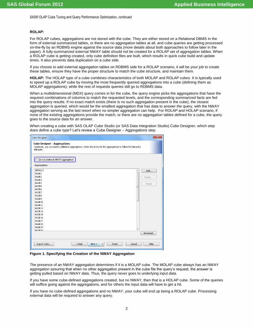
When creating a cube with SAS OLAP Cube Studio (or SAS Data Integration Studio) Cube Designer, which step does define a cube type? Let‘s review a Cube Designer – Aggregations step.

Figure 1. Specifying the Creation of the NWAY Aggregation

The presence of an NWAY aggregation determines if it is a MOLAP cube. The MOLAP cube always has an NWAY aggregation assuring that when no other aggregation present in the cube fits the query‘s request, the answer is getting pulled based on NWAY data. Thus, the query never goes to underlying input data.

If you have some cube-defined aggregations created, but no NWAY, then that is a HOLAP cube. Some of the queries will suffice going against the aggregations, and for others the input data will have to get a hit.

If you have no cube-defined aggregations and no NWAY, your cube will end up being a ROLAP cube. Processing external data will be required to answer any query.



3

The easiest aggregations to create and tune are the ones that are done for a MOLAP cube.

MOLAP AGGREGATIONS

MOLAP AGGREGATIONS – INITIAL CREATION

When a cube is first deployed to the users, you do not have a luxury of accumulated cube usage data, but you still need to provide cube users a decently performing cube. How do you approach creating the initial set of aggregations?

While ad hoc analysis patterns are hard to predict, you have to make your best guess. Ideally, for a cube design phase, you get access to information about typical reports that are in use or will be created based on this cube. Cube levels and statistics used in these reports should be considered for the first aggregations round.

Another tool that you can use for the initial set of aggregations is dimensions and levels cardinality (the number of discrete values for a cube dimension or level). You can use SAS OLAP Cube Studio Aggregation Tuning plug-in to help you analyze cardinalities. The built-in algorithm takes dimension cardinalities and relative levels cardinality within the hierarchies (roll-up ratios of hierarchy levels) into consideration when providing an aggregations recommendation. Roll-up ratios of hierarchy levels are important when you have a large cardinality low-level with a much smaller cardinality parent; in this case you want to ensure you have an aggregation for the parent crossed with all the rest of dimensions, so that you don‘t roll up low-level values every time you query for the parent. See details on using the plug-in in the next section of the paper.

MOLAP AGGREGATIONS TUNING

MOLAP aggregations tuning involves three phases:

• obtaining an ARM log

• an ARM log analysis

• updating aggregations according to ARM analysis findings

We‘ll walk through each of these phases with more details.

Obtaining an ARM log

An Application Response Measurement (ARM) log is, among other things, a record of information about queries sent to the OLAP Server

Starting with SAS 9.2, there were a number of changes introduced in a way the ARM logging is done.

Relevant to our task, the changes are as follows:

• You can activate or deactivate logging at any time. For each OLAP server invocation, an ARM log file is always getting created. If ARM logging is deactivated, the ARM log file will be empty.

• You have the flexibility of picking your ARM log file location and a name.

By default, ARM logs are placed into files:

<olap server log directory>/performance_%d_%S{pid}.arm,

For example: C:\SAS\EBIEDIEG\Lev1\SASApp\OLAPServer\Logs\ performance_2012-02-08_7224.arm

• You have a choice of activating ARM logging temporarily on a running server or permanently via OLAP Server logconfig.xml file, in which case a server restart is needed to put activation in effect.

Appendix A of this paper explains how to activate ARM logging using both approaches.

An ARM log file created for each OLAP server invocation is the file you want to keep and feed into the Aggregations Tuning plug-in for aggregations analysis. With current implementation (SAS 9.3), you can only feed one ARM log at a time.

An ARM log analysis & updating aggregations according to ARM analysis findings

The next two phases can be done using Aggregation Tuning plug-in. To access the plug-in from SAS OLAP Cube Studio, right-click on a cube and select Aggregation Tuning.



4

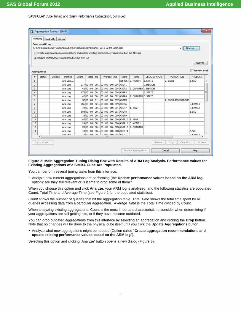
Figure 2: Main Aggregation Tuning Dialog Box with Results of ARM Log Analysis. Performance Values for Existing Aggregations of a SIMBA Cube Are Populated.

You can perform several tuning tasks from this interface:

• Analyze how current aggregations are performing (the Update performance values based on the ARM log

option): are they still relevant or is it time to drop some of them?

When you choose this option and click Analyze, your ARM log is analyzed, and the following statistics are populated:

Count, Total Time and Average Time (see Figure 2 for the populated statistics).

Count shows the number of queries that hit the aggregation table. Total Time shows the total time spent by all queries accessing data from a particular aggregation. Average Time is the Total Time divided by Count.

When analyzing existing aggregations, Count is the most important characteristic to consider when determining if your aggregations are still getting hits, or if they have become outdated.

You can drop outdated aggregations from this interface by selecting an aggregation and clicking the Drop button. Note that no changes will be done to the physical cube itself until you click the Update Aggregations button.

Analyze what new aggregations might be needed (Option called ―Create aggregation recommendations and update existing performance values based on the ARM log‖).

Selecting this option and clicking ‗Analyze‘ button opens a new dialog (Figure 3).



5

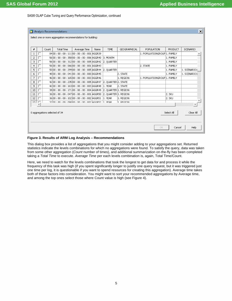
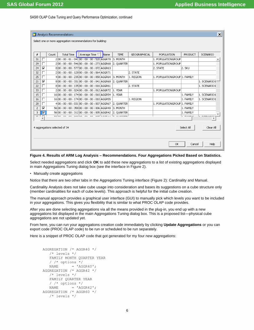
Figure 3. Results of ARM Log Analysis – Recommendations

This dialog box provides a list of aggregations that you might consider adding to your aggregations set. Returned statistics indicate the levels combinations for which no aggregations were found. To satisfy the query, data was taken from some other aggregation (Count number of times), and additional summarization on-the-fly has been completed taking a Total Time to execute. Average Time per each levels combination is, again, Total Time/Count.

Here, we need to watch for the levels combinations that took the longest to get data for and process it while the frequency of this task was high (if you spent significantly longer to justify one query request, but it was triggered just one time per log, it is questionable if you want to spend resources for creating this aggregation). Average time takes both of these factors into consideration. You might want to sort your recommended aggregations by Average time, and among the top ones select those where Count value is high (see Figure 4).



6

Figure 4. Results of ARM Log Analysis – Recommendations. Four Aggregations Picked Based on Statistics.

Select needed aggregations and click OK to add these new aggregations to a list of existing aggregations displayed

in main Aggregations Tuning dialog box (see the interface in Figure 2).

• Manually create aggregations

Notice that there are two other tabs in the Aggregations Tuning interface (Figure 2): Cardinality and Manual.

Cardinality Analysis does not take cube usage into consideration and bases its suggestions on a cube structure only (member cardinalities for each of cube levels). This approach is helpful for the initial cube creation.

The manual approach provides a graphical user interface (GUI) to manually pick which levels you want to be included in your aggregations. This gives you flexibility that is similar to what PROC OLAP code provides.

After you are done selecting aggregations via all the means provided in the plug-in, you end up with a new aggregations list displayed in the main Aggregations Tuning dialog box. This is a proposed list—physical cube aggregations are not updated yet.

From here, you can run your aggregations creation code immediately by clicking Update Aggregations or you can

export code (PROC OLAP code) to be run or scheduled to be run separately.

Here is a snippet of PROC OLAP code that got generated for my four new aggregations:

AGGREGATION /* AGGR40 */

/* levels */

FAMILY MONTH QUARTER YEAR

/ /* options */

NAME = 'AGGR40';


/* levels */

FAMILY QUARTER YEAR

/ /* options */

NAME = 'AGGR42';


/* levels */



7

QUARTER SCENARIO1 YEAR

/ /* options */

NAME = 'AGGR60';


/* levels */

FAMILY POPULATIONGROUP SKU STATE

/ /* options */

NAME = 'AGGR63';

MOLAP AGGREGATIONS PERFORMANCE OPTIONS

After you are done with the ARM log analysis and updated the aggregations set, make sure you have it in your plan to come back to this exercise on a regular basis. Empowering your MOLAP cube with a set of carefully selected aggregations is the most important step you can take to boost its querying performance. Assuming you review your selection on a regular basis, you can stop your aggregations maintenance at that.

It would be good to know though that you also have an option of adjusting aggregations parameters. Though the default settings will suit the majority of OLAP Server scenarios, you have quite a tool set to control how aggregations are created and accessed.

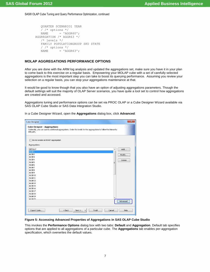
Aggregations tuning and performance options can be set via PROC OLAP or a Cube Designer Wizard available via SAS OLAP Cube Studio or SAS Data Integration Studio.

In a Cube Designer Wizard, open the Aggregations dialog box, click Advanced:

Figure 5: Accessing Advanced Properties of Aggregations in SAS OLAP Cube Studio

This invokes the Performance Options dialog box with two tabs: Default and Aggregation. Default tab specifies options that are applied to all aggregations of a particular cube. The Aggregations tab enables per-aggregation

specification, which overwrites the default values.



8

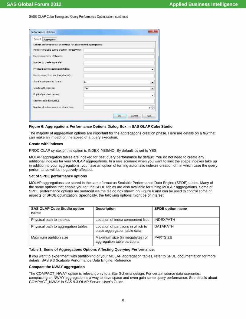
Figure 6: Aggregations Performance Options Dialog Box in SAS OLAP Cube Studio

The majority of aggregation options are important for the aggregations creation phase. Here are details on a few that can make an impact on the speed of a query execution.

Create with indexes

PROC OLAP syntax of this option is INDEX=YES/NO. By default it‘s set to YES.

MOLAP aggregation tables are indexed for best query performance by default. You do not need to create any additional indexes for your MOLAP aggregations. In a rare scenario when you want to limit the space indexes take up in addition to your aggregations, you have an option of turning automatic indexes creation off, in which case the query performance will be negatively affected.

Set of SPDE performance options

MOLAP aggregations are stored in the same format as Scalable Performance Data Engine (SPDE) tables. Many of the same options that enable you to tune SPDE tables are also available for tuning MOLAP aggregations. Some of SPDE performance options are surfaced via the dialog box shown on Figure 6 and can be used to control some of aspects of SPDE optimization. Specifically, the following options might be of interest:

SAS OLAP Cube Studio option name

Description SPDE option name

Physical path to indexes Location of index component files INDEXPATH

Physical path to aggregation tables Location of partitions in which to place aggregation table data

DATAPATH

Maximum partition size Maximum size (in megabytes) of aggregation table partitions

PARTSIZE

Table 1. Some of Aggregations Options Affecting Querying Performance.

If you want to experiment with partitioning of your MOLAP aggregation tables, refer to SPDE documentation for more details: SAS 9.3 Scalable Performance Data Engine: Reference

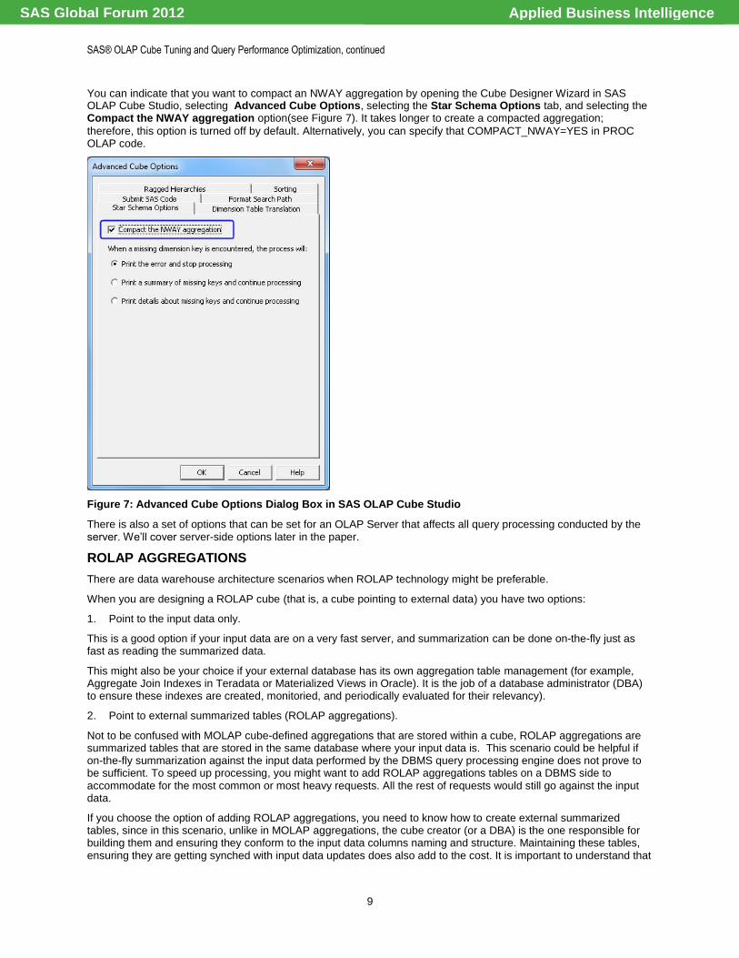
Compact the NWAY aggregation

The COMPACT_NWAY option is relevant only to a Star Schema design. For certain source data scenarios, compacting an NWAY aggregation is a way to save space and even gain some query performance. See details about COMPACT_NWAY in SAS 9.3 OLAP Server: User's Guide.



9

You can indicate that you want to compact an NWAY aggregation by opening the Cube Designer Wizard in SAS OLAP Cube Studio, selecting Advanced Cube Options, selecting the Star Schema Options tab, and selecting the Compact the NWAY aggregation option(see Figure 7). It takes longer to create a compacted aggregation;

therefore, this option is turned off by default. Alternatively, you can specify that COMPACT_NWAY=YES in PROC OLAP code.

Figure 7: Advanced Cube Options Dialog Box in SAS OLAP Cube Studio

There is also a set of options that can be set for an OLAP Server that affects all query processing conducted by the server. We‘ll cover server-side options later in the paper.

ROLAP AGGREGATIONS

There are data warehouse architecture scenarios when ROLAP technology might be preferable.

When you are designing a ROLAP cube (that is, a cube pointing to external data) you have two options:

1. Point to the input data only.

This is a good option if your input data are on a very fast server, and summarization can be done on-the-fly just as fast as reading the summarized data.

This might also be your choice if your external database has its own aggregation table management (for example, Aggregate Join Indexes in Teradata or Materialized Views in Oracle). It is the job of a database administrator (DBA) to ensure these indexes are created, monitoried, and periodically evaluated for their relevancy).

2. Point to external summarized tables (ROLAP aggregations).

Not to be confused with MOLAP cube-defined aggregations that are stored within a cube, ROLAP aggregations are summarized tables that are stored in the same database where your input data is. This scenario could be helpful if on-the-fly summarization against the input data performed by the DBMS query processing engine does not prove to be sufficient. To speed up processing, you might want to add ROLAP aggregations tables on a DBMS side to accommodate for the most common or most heavy requests. All the rest of requests would still go against the input data.

If you choose the option of adding ROLAP aggregations, you need to know how to create external summarized tables, since in this scenario, unlike in MOLAP aggregations, the cube creator (or a DBA) is the one responsible for building them and ensuring they conform to the input data columns naming and structure. Maintaining these tables, ensuring they are getting synched with input data updates does also add to the cost. It is important to understand that



10

if data in your summarized tables gets out of synch with the input data, you are risking getting different results depending on if your query does or does not hit the particular aggregation, which is a data integrity problem.

You can use PROC SUMMARY, PROC MEANS, or PROC SQL to create a summarized table for the purpose of ROLAP aggregation. Refer to the ―SAS®9 OLAP Server: Data Management for ROLAP Aggregations‖ white paper for details about and examples of creating summarized tables for a ROLAP scenario.

Unlike with MOLAP aggregations, where aggregation tables optimization is done behind the scenes (taking aggregations and server options into consideration, be that the default or overwritten options), ROLAP summarized tables should be optimized by a DBA to ensure that all the needed indexing is set on tables for the optimum DBMS query engine processing.

ROLAP query performance depends on a success of SAS SQL implicit pass-through execution, where OLAP-generated queries are getting passed down to DBMS for execution. In a successful scenario, most of processing happens close to where source data lives (DBMS), which minimizes data movement between the DBMS and SAS and takes advantage of DBMS own optimization technology; this makes a huge performance impact. If you‘re taking a ROLAP architecture route, consider learning how the SAS SQL pass-through facility operates and, possibly, the SAS in-Database offering (which, for example, enables you to push your formats down to DBMS, which increases a success rate of an implicit pass-through).

HOW TO ADD ROLAP AGGREGATIONS TO A CUBE

You can link your ROLAP (or HOLAP) cube with external aggregations either manually with PROC OLAP code or using the SAS OLAP Cube Studio (and SAS Data Integration Studio) Cube Designer interface. You cannot use the Aggregation Tuning plug-in to add ROLAP aggregations to the cube.

In PROC OLAP code, add the TABLE=<libname.external_summary_table_name> option to an AGGREGATION statement for each of the aggregation tables to link:

AGGREGATION FAMILY MONTH QUARTER YEAR / TABLE=Teralib.AGGR40;

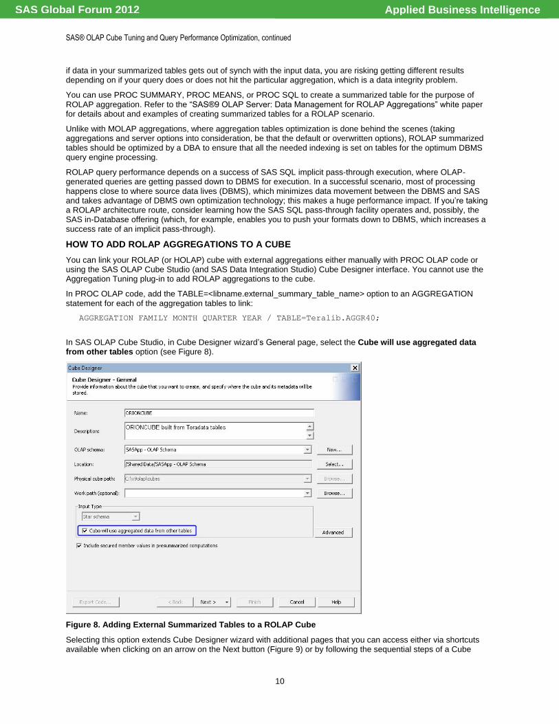
In SAS OLAP Cube Studio, in Cube Designer wizard‘s General page, select the Cube will use aggregated data from other tables option (see Figure 8).

Figure 8. Adding External Summarized Tables to a ROLAP Cube

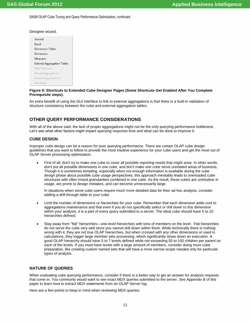
Selecting this option extends Cube Designer wizard with additional pages that you can access either via shortcuts available when clicking on an arrow on the Next button (Figure 9) or by following the sequential steps of a Cube



11

Designer wizard.

Figure 9: Shortcuts to Extended Cube Designer Pages (Some Shortcuts Get Enabled After You Complete Prerequisite steps).

An extra benefit of using the GUI interface to link to external aggregations is that there is a built-in validation of structure consistency between the cube and external aggregation tables.

OTHER QUERY PERFORMANCE CONSIDERATIONS

With all of the above said, the lack of proper aggregations might not be the only querying performance bottleneck. Let‘s see what other factors might impact querying response time and what can be done to improve it.

CUBE DESIGN

Improper cube design can be a reason for poor querying performance. There are certain OLAP cube design guidelines that you want to follow to provide the most intuitive experience for your cube users and get the most out of OLAP Server processing optimization.

First of all, don't try to make one cube to cover all possible reporting needs that might arise. In other words, don't put all possible dimensions in one cube, and don't make one cube serve unrelated areas of business. Though it is sometimes tempting, especially when not enough information is available during the cube design phase about possible cube usage perspectives, this approach inevitably leads to overloaded cube structures with often mixed granularities combined in one cube. As the result, these cubes are unintuitive in usage, are prone to design mistakes, and can become unnecessarily large.

In situations when some cube users require much more detailed data for their ad hoc analysis, consider adding a drill-through table to your cube.

Limit the number of dimensions or hierarchies for your cube. Remember that each dimension adds cost to aggregations maintenance and that even if you do not specifically select or drill down to this dimension within your analysis, it is a part of every query submitted to a server. The ideal cube should have 5 to 10 hierarchies defined.

Stay away from "flat" hierarchies—one-level hierarchies with tons of members on the level. Flat hierarchies do not serve the cube very well since you cannot drill down within them. While technically there is nothing wrong with it, they are not true OLAP hierarchies, but when crossed with any other dimensions or used in calculations, they trigger large member sets processing, which significantly slows down an execution. A good OLAP hierarchy should have 5 to 7 levels defined while not exceeding 50 to 100 children per parent on each of the levels. If you must have levels with a large amount of members, consider doing more cube preparation, like creating custom named sets that will have a more narrow scope needed only for particular types of analysis.

NATURE OF QUERIES

When evaluating cube querying performance, consider if there is a better way to get an answer for analysis requests that come in. You commonly would want to see exact MDX queries submitted to the server. See Appendix B of this paper to learn how to extract MDX statements from an OLAP Server log.

Here are a few points to keep in mind when reviewing MDX queries:



12

MDX is a rich language for querying multidimensional data. Often, there are several ways to accomplish the same analysis task with different MDX techniques, with some performing more efficiently than others. If possible, you might want to experiment rewriting your queries for ad hoc requests or suggest different reporting layouts or filtering parameters if requests are coming from a reporting client MDX generator.

Efficiency becomes even more critical when adding custom calculations (calculated members) to your cube. While tweaking the nature of users' reporting requests is something you usually have limited control over, custom calculations defined on a cube level are in the hands of a cube designer or administrator. Custom calculations can sometimes become expensive. Unlike cube-defined measures, custom calculations are not getting pre-aggregated and are getting processed on-the-fly during the query execution. Be mindful of this factor when introducing large sets manipulations that can trigger an excessive number of subqueries to be run on a server.

See more details about adding calculations to your cube in ―How to Customize Your Data Analysis with SAS® OLAP Cube Calculations‖ white paper.

OLAP SERVER OPTIONS FOR QUERYING PERFORMANCE

Earlier, we reviewed what options can be set for a cube that affect the creation and processing of aggregations. Those options are associated with the particular cube and, if specified, with particular aggregations.

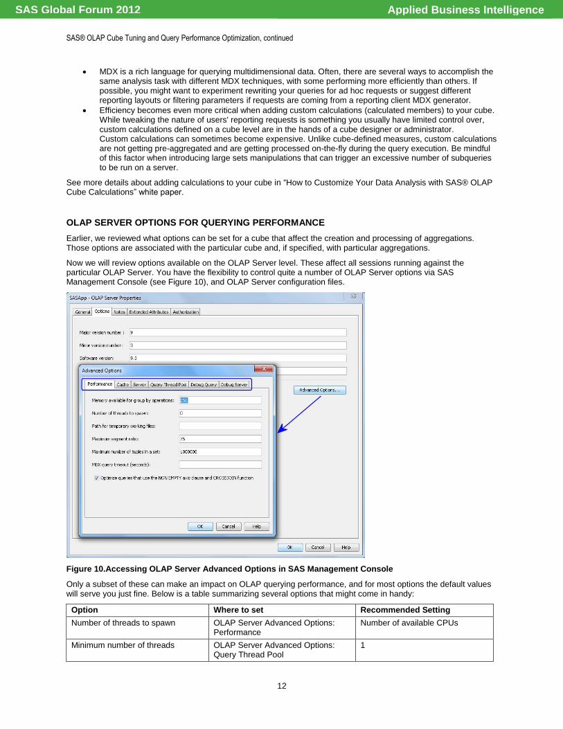
Now we will review options available on the OLAP Server level. These affect all sessions running against the particular OLAP Server. You have the flexibility to control quite a number of OLAP Server options via SAS Management Console (see Figure 10), and OLAP Server configuration files.

Figure 10.Accessing OLAP Server Advanced Options in SAS Management Console

Only a subset of these can make an impact on OLAP querying performance, and for most options the default values will serve you just fine. Below is a table summarizing several options that might come in handy:

Option Where to set Recommended Setting

Number of threads to spawn OLAP Server Advanced Options: Performance

Number of available CPUs

Minimum number of threads OLAP Server Advanced Options: Query Thread Pool

1



13

Option Where to set Recommended Setting

Maximum number of threads OLAP Server Advanced Options: Query Thread Pool

2 * Number of available CPUs, or even lower

Subquery cache: memory size for subquery cache

OLAP Server Advanced Options: Cache

Default value: 5MB

Subquery cache: cache the empty subquery result sets

OLAP Server Advanced Options: Cache

Default value: OFF

Maximum number of flattened rows OLAP Server Advanced Options: Server

Depends on analysis needs

Optimize queries that use the NON EMPTY axis clause and CROSSJOIN function

OLAP Server Advanced Options: Performance

Default value: ON

Memsize OLAP Server: Configuration file The more the better, but avoid causing resources contention by concurrent processes

Table 2. Some of Advanced OLAP Server Options Affecting Querying Performance.

Thread settings in greater detail

You'd expect to see measurable effects from setting thread options during concurrent query execution.

The Query Thread Pool settings in particular have an effect only for multiple concurrent query requests. The recommended values are geared to provide the best multi-user performance and scalability. If you are running as a single user, you will not see any performance difference, no matter how those values are set.

The Maximum number of threads setting controls how many MDX queries can be executed in parallel by the

server. For example, if this option is set to 1, the server will execute only one MDX query at a time. If other queries come in while the current one is still executing, they‘ll wait to start until the current one is finished. Setting a maximum value (suggested value is two concurrent MDX queries per CPU) is making sure that the server doesn‘t run out of resources in multi-user situations. Consider, for example, that the maximum value is set to 8, and you have more than 8 concurrent MDX queries. Some of the queries might have some wait time, but all of them have a chance to finish rather than fighting for starved CPU resources or running out of memory. If you notice low CPU and memory utilization during high user concurrency, increasing the query thread pool maximum value is something to consider.

The Minimum number of threads controls the internal thread cache. If the value is 1, the server will free each

thread after use. If the value is higher, the server will keep that number of threads active, ready to be re-used by the next query. The smaller the value, the more free memory you have at any given time. The bigger the value, the smaller the likelihood that a new query will have to allocate a new thread from the thread pool.

Subquery Cache: Memory size for subquery cache

The subquery cache stores intermediate results during query processing. Each query has its own subquery cache. The memory setting is a maximum—it's not pre-allocated for each query and is only allocated if available. When no more free memory is available, or when the limit is reached, disk I/O is used. Lowering this value should free up memory for other purposes but possibly at the cost of lower performance.

Increasing this value could speed things up, but might interfere with the memory available for processing (leading to out-of-memory conditions) or the data cache.

Subquery Cache: Cache the empty subquery result sets

Most of the set processing in OLAP queries deals with highly sparse matrixes. By default, the subquery cache holds only the non-empty cells. Caching the empty results can make navigating the result matrix faster, but at the cost of potentially large amounts of memory. This option might help speed up processing if plenty of extra memory is available and if the cube or the queries are reasonably dense.

Maximum number of flattened rows

This option limits the amount of detailed data returned for drill-through queries. Drill-through queries on large data are costly. Depending on analysis needs, it could be that a sample of data is all that the cube user requires. If this is the case, you can set this option to limit the number of records returned. By default it‘s set to 300,000 rows.

Optimize queries that use the NON EMPTY axis clause and CROSSJOIN function



14

NON EMPTY Crossjoin is a common function in MDX queries that is used to compress results returned from multidimensional sets. This option controls how NON EMPTY Crossjoins are handled. In almost all cases, the optimized processing is faster than the non-optimized processing, although it generates more subqueries as the result. Optimization is set ON by default.

Memsize

The SAS system option MEMSIZE is the only option that controls how much memory is available to the OLAP Server process as a whole. We recommend setting it to the amount of available physical memory, but watch for concurrent processes running on the same machine not to cause resources contention.

MEMSIZE option can be set in SAS configuration file sasv9.cfg in OLAP Server configuration directory.

Please note that the SAS system option REALMEMSIZE does NOT have any effect on the OLAP Server cube querying. It does for the cube building.

Please note also that the SAS system option CPUCOUNT does NOT have any effect on the OLAP Server.

Whenever you update OLAP Server options, you need to restart the server to pick them up.

INPUT/OUTPUT SUBSYSTEM

OLAP Server jobs are known to be Input/Output-intensive for both cube creation and querying. When you evaluate OLAP cube performance requirements, don‘t underestimate the criticality of supporting OLAP operations with a sufficient I/O subsystem. The minimal throughput of the I/O subsystem should be no less than 50 to 75MBs/sec per CPU.

MULTI-USER SCALABILITY

It could be that the architecture does not keep up with the growing number of concurrent OLAP users. The solution to this, in addition to keeping your hardware in accordance with expanding needs, might be to balance OLAP querying load over several machines, each running a load-balanced OLAP Server. OLAP Server load balancing won‘t solve a problem if particular queries take too long to run, but it is aimed to make your server scalable in a multi-user environment; a load-balancing algorithm will route each newly open OLAP connection to go on the least busy server. You can find information on OLAP Server load-balancing set up in ―Enhancements for Managing SAS® OLAP Server in SAS® 9.2.‖ white paper.

CONCLUSION

Tuning cube for querying performance is a balancing act: too few aggregations would prevent you from exercising the full power of OLAP querying, while too many aggregations take storage space and affect cube building performance. Creating an aggregations set that would bring the most value for the particular cube analysis requirements is an art a cube designer needs to master. Keeping this aggregation package aligned with evolving cube querying patterns is yet another responsibility of the cube designer or BI administrator.

While tuning cube aggregations is the one most effective technique for controlling OLAP querying performance, there are other factors that have an impact and that need to be examined when searching for potential performance improvement. Determine whether your cube structural design conforms to the best OLAP design guidelines or whether your custom calculations can be done more effectively. If you are dealing with large cubes and large user base, did you consider load-balancing your OLAP server processing and partitioning of your cube aggregations? And an obvious, but no less critical factor, is ensuring that a system architecture is in place that is ready for the demands placed upon it.

APPENDIX A: ACTIVATING ARM LOGGING FOR AN OLAP SERVER

Activating ARM logging temporarily on a running OLAP Server

In SAS Management Console, select the physical OLAP Server. In right pane, select the Logger tab where you'll

have a list of all available Loggers (You should be connected to this server to see all the tabs populated. If you‘re not, right-click on the OLAP server and select Connect).



15

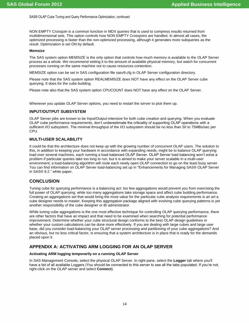
Figure 11: SAS Management Console – Configuring OLAP Server Logger

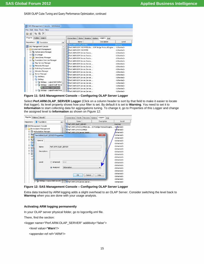
Select Perf.ARM.OLAP_SERVER Logger (Click on a column header to sort by that field to make it easier to locate that logger). Its level property shows how your filter is set. By default it is set to Warning. You need to set it to Information to start collecting data for aggregations tuning. To change it, go to Properties of this Logger and change the assigned level to Information as shown on Figure 12:

Figure 12: SAS Management Console – Configuring OLAP Server Logger

Extra data tracked by ARM logging adds a slight overhead to an OLAP Server. Consider switching the level back to Warning when you are done with your usage analysis.

Activating ARM logging permanently

In your OLAP server physical folder, go to logconfig.xml file.

There, find the section:

<logger name="Perf.ARM.OLAP_SERVER" additivity="false">

<level value="Warn"/>

<appender-ref ref="ARM"/>



16

</logger>

And update level value to "Info".

Note: The same config file has a location specified where your arm log is stored. You can update it if needed.



<appender name="ARM2LOG" class="FileAppender">

<param name="fileNamePattern" value="C:\SAS\EBIEDIEG\Lev1\SASApp\OLAPServer\Logs\performance_St_%d_%S{pid}.arm"/>

After the change is been made, restart your OLAP Server.

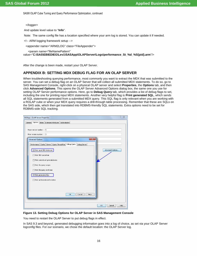
APPENDIX B: SETTING MDX DEBUG FLAG FOR AN OLAP SERVER

When troubleshooting querying performance, most commonly you want to extract the MDX that was submitted to the server. You can set a debug flag on an OLAP Server that will collect all submitted MDX statements. To do so, go to SAS Management Console, right-click on a physical OLAP server and select Properties, the Options tab, and then click Advanced Options. This opens the OLAP Server Advanced Options dialog box, the same one you use for setting OLAP Server performance options. Here, go to Debug Query tab, which provides a list of debug flags to set, including the one for printing input MDX statements. Another very helpful flag is Print generated SQL, which sends

all SQL statements generated from a submitted MDX query. This SQL flag is only relevant when you are working with a ROLAP cube or when your MDX query requires a drill-through table processing. Remember that these are SQLs on the SAS side, which then get translated into RDBMS-friendly SQL statements. Extra options need to be set for RDBMS-side SQL tracking.

Figure 13. Setting Debug Options for OLAP Server in SAS Management Console

You need to restart the OLAP Server to put debug flags in effect.

In SAS 9.3 and beyond, generated debugging information goes into a log of choice, as set via your OLAP Server logconfig files. For our scenario, we chose the default location: the OLAP Server log.



17

C:\SAS\EBIEDIEG\Lev1\SASApp\OLAPServer\Logs\SASApp_OLAPServer_2012-02-20_l73618_12604.log

Before SAS 9.3, this information used to go to SSNJ<nnnnn> files in the OLAP Server startup directory with a separate file created for each OLAP Server session.

Remember to turn extra debugging OFF when done with your performance analysis and tuning. Tracking extra debugging information can become I/O intensive.

REFERENCES AND RECOMMENDED READING

―SAS 9 OLAP Server: Data Management for ROLAP Aggregations.‖ Cary, NC: SAS Institute. Available at http://support.sas.com/resources/papers/ROLAPDataManagement.pdf.

Simmons, Mary, and Michelle Wilkie. 2009. ―Best Practice: Optimizing the cube build process in SAS® 9.2.‖ Proceedings of the SAS Global Forum 2009 Conference. Cary, NC: SAS Institute. Available at

http://support.sas.com/resources/papers/proceedings09/319-2009.pdf.

Petrova, Tatyana. 2011. ―How to Customize Your Data Analysis with SAS® OLAP Cube Calculations.‖ Proceedings of the SAS Global Forum 2011 Conference. Cary, NC: SAS Institute. Available at http://support.sas.com/resources/papers/proceedings11/043-2011.pdf.

Ender, Matthias, and Tatyana Petrova. 2010. ―Enhancements for Managing SAS® OLAP Server in SAS® 9.2.‖ Proceedings of the SAS Global Forum 2010 Conference. Cary, NC: SAS Institute. Available at http://support.sas.com/resources/papers/proceedings10/330-2010.pdf.

Wilkie, Michelle, Mary Simmons, et al. 2009. ―Using SAS® OLAP Server for a ROLAP Scenario.‖ Proceedings of the SAS Global Forum 2009 Conference. Cary, NC: SAS Institute. Available at http://support.sas.com/resources/papers/proceedings09/103-2009.pdf.

SAS Institute. 2011. SAS® 9.3 OLAP Server: User's Guide. Cary, NC: SAS Institute.

SAS Institute. 2011. ―Understanding the ARM Records Written for SAS OLAP Server.‖ In SAS® 9.3 Interface to Application Response Measurement (ARM): Reference. 49–56. Cary, NC: SAS Institute.

SAS Institute. 2011. ―SPD Engine LIBNAME Statement Options.‖ In SAS® 9.3 Scalable Performance Data Engine: Reference. 23–38. Cary, NC: SAS Institute.

Kimball, Ralph, Margy Ross, et al. 2008. The Data Warehouse Lifecycle Toolkit. Indianapolis, Indiana: Wiley Publishing, Inc.

ACKNOWLEDGMENTS

Acknowledgments go to Matthias Ender at SAS Institute Inc. for his continuous effort in documenting SAS OLAP Server tips and techniques and for a thorough review of this paper.

CONTACT INFORMATION

Your comments and questions are valued and encouraged. Contact the author at:

Tatyana Petrova SAS Institute Inc. SAS Campus Drive, Cary, NC [email protected]

SAS and all other SAS Institute Inc. product or service names are registered trademarks or trademarks of SAS Institute Inc. in the USA and other countries. ® indicates USA registration.

Other brand and product names are trademarks of their respective companies.


http://support.sas.com/resources/papers/ROLAPDataManagement.pdf

http://support.sas.com/resources/papers/proceedings09/319-2009.pdf




mailto:[email protected]

Documents

026-2012: SAS® OLAP Cube Tuning and Query Performance Optimizationsupport.sas.com/resources/papers/proceedings12/026-2012.pdf · 2012-04-02 · 1 Paper 026-2012 SAS® OLAP Cube Tuning